Average Intensity of a Laguerre—Gaussian Vector Vortex Beam through Inhomogeneous Atmospheric Turbulence

Abstract

We investigate the evolution properties of a partially coherent Laguerre–Gaussian vector vortex (LGVV) beam through inhomogeneous atmospheric turbulence. Analytical formulae for the elements of a cross-spectral density matrix of a partially coherent LGVV beam propagating in turbulence are derived with the help of the extended Huygens–Fresnel principle. Our outcomes demonstrate that the normalized initial profile of a partially coherent beam with concentric dark rings gradually evolves into a Gaussian-like beam profile in turbulence. We also find that the beam is emitted at a large zenith angle and quickly converts to a Gaussian-like beam. Furthermore, it is also shown that a propagation beam with a large topological charge has a stronger ability to resist atmospheric turbulence. In order to confirm our numerical results, we combine the complex screen method and multi-phase screen method to simulate the propagation of a partially coherent LGVV beam in atmospheric turbulence. It is indicated that the simulation results are in good agreement with theoretical predictions. Our results will pave the way for the development of free-space optical communications and remote sensing.

1. Introduction

In the past decades, numerous efforts have been devoted to the propagation of partially coherent (PC) beams in atmospheric turbulence due to their important applications in free-space optical communications, lidar distance measurement and remote sensing [1,2,3,4,5,6,7,8,9,10,11,12,13,14,15]. It is generally considered that atmospheric turbulence causes a series of harmful turbulence effects such as scintillation (i.e., intensity fluctuation), phase distortion and so on, which will lead to an increase in the communication error rate and decrease in the channel capacity of the system [1,2,3,4,5]. Therefore, it is of practical importance to develop a method to overcome or reduce turbulence effects. It is demonstrated that one may use special beams to achieve this goal [6,7,8,9,10,11,12,13,14,15]. A PC beam is more suitable for propagation in turbulent media than a fully coherent beam because it is less affected by turbulent media and can effectively mitigate harmful optical phenomena such as beam spreading, drift, scintillation, speckles and uneven intensity distribution [6,7,8,9,10,11,12,13]. In 2003, Shirai et al. explained the reason using a coherent-mode representation of the spreading of partially coherent beams propagating through atmospheric turbulence [3]. In 1992, Allen et. al. found that each photon in a beam with a phase factor exp(imθ) has an orbital angular momentum (OAM) of ħm, where m is the topological charge carried by the beam and ħ is the reduced Planck constant. And this kind of beam with OAM is called a vortex beam [16,17,18,19], which can reduce the effect of turbulence. Furthermore, PC beams with special spatial structures, such as radially polarized (RP) beams [6,7,8,9,10,11], partially coherent vortex (PCV) beams [9,10,11,12,13,16,17,18,19], partially coherent Laguerre–Gaussian vortex (PCLGV) beams, partially coherent radially polarized Laguerre–Gaussian vortex (PCRPLGV) beams [10], partially coherent twisted (PCT) beams, partially coherent twisted vortex (PCTV) beams [14,15] and so on, can also effectively reduce the effect of turbulence. These special beams have a common characteristic: when they propagate in inhomogeneous atmospheric turbulence, the beam quality is better than that of fundamental mode Gaussian beams, and the evolution of the distribution of these beams during propagation in inhomogeneous atmospheric turbulence is slower, with stronger resistance to atmospheric turbulence, such as the ability of PCV beams, PCLGV beams, PCRPLGV beams and PCTV beams to maintain a hollow distribution during long-distance transmission [9,10,11,12,13,14,15,16].

On the other hand, the propagation of most beams in atmospheric turbulence is often assumed to be horizontal (i.e., the structural parameter of the refractive-index fluctuation in turbulence is treated as a constant). However, for some special applications (e.g., lidar detection and imaging, remote sensing), these beams propagate in atmospheric turbulence along a slant path, and the structural parameter of the refractive-index fluctuation in turbulence is variable [4,6,12,20,21,22,23,24,25]. As is well known, in the practical applications of LiDAR (including ground-based LiDAR or vehicular LiDAR) in atmospheric detection and imaging, laser satellite ranging and lunar laser ranging, the intensity of atmospheric turbulence changes with transformation of ground height and induces variation in the phase structure of the emitted beam. Therefore, studying the propagation characteristics of partially coherent special structure beams in atmospheric turbulence should consider turbulence to be inhomogeneous atmospheric turbulence.

Up to now, to the best of our knowledge, the average intensity of a partially coherent Laguerre–Gaussian vector vortex (LGVV) beam through inhomogeneous atmospheric turbulence has not been reported. In this paper, we first derive the analytical formulae for the elements of the cross-spectral density matrix of a partially coherent LGVV beam propagating in turbulence with the help of the extended Huygens–Fresnel principle, then we study the evolution laws of the average intensity of partially coherent beams in turbulence, analyze the effect of beam parameters and turbulence parameters on them and obtain the main parameters that affect the average intensity distribution of partially coherent beams propagating through inhomogeneous atmospheric turbulence. Finally, we use the multi-phase screen method to confirm our theoretical results and show that the simulation results are in good agreement with theoretical predictions; we also find that the accuracy of the physical image is related to the number and interval of phase screens. These results are of interest for the optimization of earth-satellite communications and imaging links as well as in astronomical studies.

2. Theoretical Model

The electric field of a full coherent LGVV beam in cartesian coordinates is expressed as [9,10,11]:

$$\begin{array}{cc}E\left(r;0\right)& =\frac{x}{w_0}\exp \left(-\frac{r^2}{w_0^2}\right)\frac{{\left(-1\right)}^n}{2^{2n+m}n!}{\displaystyle \sum _{t=0}^n{\displaystyle \sum _{s=0}^m{i}^s\left(\begin{array}{c}n\\ t\end{array}\right)\left(\begin{array}{c}m\\ s\end{array}\right)}}{H}_{2t+m-s}\left(\frac{\sqrt{2}x}{w_0}\right)H_{2n-2t+s}\left(\frac{\sqrt{2}y}{w_0}\right)e_x\\ & +\frac{y}{w_0}\exp \left(-\frac{r^2}{w_0^2}\right)\frac{{\left(-1\right)}^n}{2^{2n+m}n!}{\displaystyle \sum _{t=0}^n{\displaystyle \sum _{s=0}^m{i}^s\left(\begin{array}{c}n\\ t\end{array}\right)\left(\begin{array}{c}m\\ s\end{array}\right)}}{H}_{2t+m-s}\left(\frac{\sqrt{2}x}{w_0}\right)H_{2n-2t+s}\left(\frac{\sqrt{2}y}{w_0}\right)e_y,\end{array}$$

(1)

where r = (x, y) is an arbitrary transverse position vector in the initial plane, w₀ represents the beam waist for the fundamental Gaussian beam, m and n denote the topological charge number and the radial index, respectively, and e_x and e_y are the unit vectors in the x and y directions, respectively. H_2t+m−s(·) and H_2n−2t+s(·) are the Hermitian polynomials; we use their summation form to represent the Laguerre term in the original LGVV beam expression [14,15,26,27,28,29,30]. And $\left(\begin{array}{c}n\\ t\end{array}\right)$ and $\left(\begin{array}{c}m\\ s\end{array}\right)$ are the binomial coefficients.

Then, we extend the beam to a partially coherent form and consider that its coherent structure satisfies a Gaussian distribution. Its second-order statistical properties are characterized by a 2 × 2 cross-spectral density matrix (CSDM) as [9,10,11]:

$$\overleftrightarrow{W}\left({\mathit{r}}_1,{\mathit{r}}_2;0\right)=\left[\begin{array}{cc}{W}_{xx}\left({\mathit{r}}_1,{\mathit{r}}_2;0\right)& W_{xy}\left({\mathit{r}}_1,{\mathit{r}}_2;0\right)\\ W_{yx}\left({\mathit{r}}_1,{\mathit{r}}_2;0\right)& W_{yy}\left({\mathit{r}}_1,{\mathit{r}}_2;0\right)\end{array}\right],$$

(2)

where r₁ = (x₁, y₁) and r₂ = (x₂, y₂) are two arbitrary transverse position vectors in source plane (z = 0). The elements W_xx(r₁,r₂;0), W_xy(r₁,r₂;0), W_yx(r₁,r₂;0) and W_yy(r₁,r₂;0) of the CSDM for a partially coherent LGVV beam in the initial plane can be written as the following expressions [9,10,11]:

$$\begin{array}{cc}{W}_{\alpha \beta }\left({\mathit{r}}_1,{\mathit{r}}_2,0\right)& ={〈E_{\alpha }\left({\mathit{r}}_1,0\right)E_{\beta }^{\ast }\left({\mathit{r}}_2,0\right)〉}_m\\ & =\frac{{\alpha }_1{\beta }_2}{w_0^2}\exp \left(-\frac{r_1^2+r_2^2}{w_0^2}\right)\exp \left[-\frac{{\left({\mathit{r}}_1-{\mathit{r}}_2\right)}^2}{2{\delta }_{\alpha \beta }^2}\right]\frac{1}{2^{4n+2m}{\left(n!\right)}^2}{\displaystyle \sum _{t=0}^n{\displaystyle \sum _{s=0}^m{\displaystyle \sum _{\mu =0}^n{\displaystyle \sum _{\nu =0}^m{\left(i^s\right)}^{*}{i}^v}}}}\\ & \left(\begin{array}{c}n\\ t\end{array}\right)\left(\begin{array}{c}m\\ s\end{array}\right)\left(\begin{array}{c}n\\ \mu \end{array}\right)\left(\begin{array}{c}m\\ \nu \end{array}\right)H_{2t+m-s}\left(\frac{\sqrt{2}{x}_1}{w_0}\right)H_{2\mu +m-\nu }\left(\frac{\sqrt{2}{x}_2}{w_0}\right)H_{2n-2t+s}\left(\frac{\sqrt{2}{y}_1}{w_0}\right)H_{2n-2\mu +\nu }\left(\frac{\sqrt{2}{y}_2}{w_0}\right),\end{array}$$

(3)

where E_x and E_y are the two components of the stochastic electric vector in the x and y directions, respectively, α, β = x, y. 〈·〉_m denotes the ensemble average and ‘*’ represents the complex conjugate. δ_αβ represents the initial auto-correlation lengths (when α = β) and the initial mutual correlation lengths (when α ≠ β), respectively. And here, in order to calculate conveniently, in this paper, we set δ_xx = δ_yy = δ_xy = δ_yx = δ₀. Equation (3), especially, reduces to the cross-spectral density (CSD) W_αβ(r₁,r₂;0) of a radially polarized vortex beam for n = 0 and m ≠ 0, a radially polarized hollow beam for m = 0 and n ≠ 0 and a radially polarized beam for n = 0 and m = 0, respectively.

With the validity of approximate paraxial solutions, the elements of CSDM for a partially coherent LGVV beam propagating through inhomogeneous atmospheric turbulence can be related with those in the source plane with the help of the following extended Huygens–Fresnel principle integral formula [31,32,33,34,35]:

$$\begin{array}{cc}{W}_{\alpha \beta }\left({\mathit{\rho }}_1,{\mathit{\rho }}_2;z\right)& =\frac{1}{{\lambda }^2{z}^2}{\displaystyle \iint {\displaystyle \iint W_{\alpha \beta }\left({\mathit{r}}_1,{\mathit{r}}_2,0\right)}}\\ & \times \exp \left\{-\frac{ik}{2z}\left[{\left({\mathit{\rho }}_1-{\mathit{r}}_1\right)}^2-{\left({\mathit{\rho }}_2-{\mathit{r}}_2\right)}^2\right]-\frac{1}{2}{D}_w\left({\mathit{r}}_1-{\mathit{r}}_2,{\mathit{\rho }}_1-{\mathit{\rho }}_2;z\right)\right\}{d}^2{\mathit{r}}_1{d}^2{\mathit{r}}_2,\end{array}$$

(4)

W = where ρ₁ = (ρ_x1, ρ_y1) and ρ₂ = (ρ_x2, ρ_y2) are positions of two points in the received plane, k = 2π/λ represents the wave number with λ being the wavelength and z denotes the propagation distance of a partially coherent LGVV beam propagating through inhomogeneous atmospheric turbulence. D_w (r₁ − r₂, ρ₁ − ρ₂; z), which is a two-point spherical wave structure function containing the effect of inhomogeneous atmospheric turbulence, is given by [20,21,22,23,24,25]:

$$\begin{array}{cc}{D}_w\left({\mathit{r}}_1-{\mathit{r}}_2,{\mathit{\rho }}_1-{\mathit{\rho }}_2;z\right)& =\frac{8{\pi }^2{k}^2}{\cos \left(\gamma \right)}{\displaystyle {\int }_{h_0}^{H}dh}{\displaystyle {\int }_0^{\infty }\left\{1-J_0\left[\mathit{\kappa }\left|\zeta \left({\mathit{r}}_1-{\mathit{r}}_2\right)+\left(1-\zeta \right)\left({\mathit{\rho }}_1-{\mathit{\rho }}_2\right)\right|\right]\right\}}\\ & \times {\Phi }_n\left(\mathit{\kappa },h\right)\mathit{\kappa }d\mathit{\kappa },\end{array}$$

(5)

where γ is the zenith angle, J₀(·) is the zero-order Bessel function of the first kind and Φ_n(κ, h) = ${\tilde{C}}_{2_n}$(h)Φ′_n(κ) represents the spatial power spectrum of the refractive-index fluctuations in inhomogeneous atmospheric turbulence, with κ and h denoting the spatial wavenumber and propagation height, respectively. ${\tilde{C}}_{2_n}$(h) is the generalized refractive-index structural parameter varying with propagation height h. H is the height between the receiving plane and the ground, and h₀ is the height between the light source plane and the ground. In general, we consider that the light source is on the ground, that is, h₀ = 0. And ζ = 1 − h/[zcos(γ)] denotes the normalized distance variable with z = H/cos(γ) being the total propagation distance along a slant path [4,20,21,22,23,24,25].

In Equation (5), we consider the first-order approximation of J₀(·); then, Equation (5) can be rewritten as:

$$D_w\left({\mathit{r}}_1-{\mathit{r}}_2,{\mathit{\rho }}_1-{\mathit{\rho }}_2;z\right)\approx B_1{\left({\mathit{\rho }}_1-{\mathit{\rho }}_2\right)}^2+B_2\left({\mathit{\rho }}_1-{\mathit{\rho }}_2\right)\left({\mathit{r}}_1-{\mathit{r}}_2\right)+B_3{\left({\mathit{r}}_1-{\mathit{r}}_2\right)}^2,$$

(6)

where

$$B_1=\frac{2{\pi }^2{k}^2}{\cos \gamma }T\times {\displaystyle {\int }_{h_0}^H{\left(1-\zeta \right)}^2{C}_n^2\left(h\right)dh},$$

(7)

$$B_2=\frac{2{\pi }^2{k}^2}{\cos \gamma }T\times {\displaystyle {\int }_{h_0}^{H}2\left(1-\zeta \right)\zeta C_n^2\left(h\right)dh},$$

(8)

$$B_3=\frac{2{\pi }^2{k}^2}{\cos \gamma }T\times {\displaystyle {\int }_{h_0}^H{\zeta }^2{C}_n^2\left(h\right)dh},$$

(9)

$$T={\displaystyle {\int }_0^{\infty }{\kappa }^3{{\Phi }^{\prime }}_n\left(\kappa \right)}d\kappa .$$

(10)

The average intensity of a partially coherent LGVV beam propagating through inhomogeneous atmospheric turbulence is given by:

$$I\left(\mathit{\rho },\mathit{\rho };z\right)=W_{xx}\left(\mathit{\rho },\mathit{\rho };z\right)+W_{yy}\left(\mathit{\rho },\mathit{\rho };z\right),$$

(11)

We set ρ₁ = ρ₂ = ρ = (ρ_x, ρ_y); so, Equation (4) can be simplified as:

$$\begin{array}{cc}{W}_{\alpha \beta }\left(\mathit{\rho },\mathit{\rho };z\right)& =\frac{1}{{\lambda }^2{z}^2}{\displaystyle \iint {\displaystyle \iint W_{\alpha \beta }\left({\mathit{r}}_1,{\mathit{r}}_2;0\right)}}\\ & \times \exp \left[-\frac{ik}{2z}\left[{\left({\mathit{\rho }}_1-{\mathit{r}}_1\right)}^2-{\left({\mathit{\rho }}_2-{\mathit{r}}_2\right)}^2\right]-\frac{B_3{\left({\mathit{r}}_1-{\mathit{r}}_2\right)}^2}{2}\right]d^2{\mathit{r}}_1{d}^2{\mathit{r}}_2,\end{array}$$

(12)

By substituting Equation (3) into Equation (12), after the tedious integral, the analytical formulas for W_xx (ρ, ρ; z) and W_yy (ρ, ρ; z) of a partially coherent LGVV beam through inhomogeneous atmospheric turbulence can be obtained with the following expressions:

$$\begin{array}{l}{W}_{xx}\left(\mathit{\rho },\mathit{\rho };z\right)={\left(\frac{k}{2z{w}_0}\right)}^2\frac{1}{2^{4n+2m}{\left(n!\right)}^2}{\displaystyle \sum _{t=0}^n{\displaystyle \sum _{s=0}^m{\displaystyle \sum _{\mu =0}^n{\displaystyle \sum _{\nu =0}^m{\left(i^s\right)}^{\ast }{i}^{\nu }}}}}\left(\begin{array}{c}n\\ t\end{array}\right)\left(\begin{array}{c}m\\ s\end{array}\right)\left(\begin{array}{c}n\\ \mu \end{array}\right)\left(\begin{array}{c}m\\ \nu \end{array}\right)\\ {\displaystyle \sum _{a=0}^{\left[\left(2t+m-s\right)/2\right]}{\displaystyle \sum _{b=0}^{2t+m-s-2a+1}{\displaystyle \sum _{c=0}^{\left[b/2\right]}{\displaystyle \sum _{d=0}^{\left[\left(2\mu +m-\nu \right)/2\right]}{\displaystyle \sum _{e=0}^{2n-2t+s}{\displaystyle \sum _{f=0}^{\left[e/2\right]}{\displaystyle \sum _{g=0}^{\left[\left(2n-2\mu +\nu \right)/2\right]}\left(\begin{array}{c}2t+m-s-2a+1\\ b\end{array}\right)\left(\begin{array}{c}2n-2t+s\\ e\end{array}\right)}}}}}}}\\ \frac{{\left(i\right)}^{-2m-2n+s-2t+4a+2c+4d-e+4f+4g-2}b!e!\left(2t+m-s\right)!\left(2\mu +m-\nu \right)!\left(2n-2\mu +\nu \right)!}{a!c!d!f!g!\left(b-2c\right)!\left(e-2f\right)!\left(2t+m-s-2a\right)!\left(2\mu +m-\nu -2d\right)!\left(2n-2\mu +\nu -2g\right)!}\\ {\sqrt{2}}^{-m-2n+2a-b+2c-e+2f-5}{\left(\frac{\sqrt{2}}{w_0}\right)}^{2m+4n-2a-2d-2g}{\left(\frac{1}{\sqrt{A}}\right)}^{m+4n+s-2t-2a+b-2c+3}\\ {\left(\frac{1}{\sqrt{A^2{w}_0^2/2-A}}\right)}^{-2n-s+2t+e-2f}{\left(B\right)}^{b-2c+e-2f}{\left(\frac{1}{\sqrt{D}}\right)}^{m+2n+b-2c-2d+e-2f-2g+3}\\ \times \exp \left(\frac{C_{1x}^2}{4A}\right)\exp \left(\frac{E^2}{4D}\right)\exp \left(\frac{C_{1y}^2}{4A}\right)\exp \left(\frac{F^2}{4D}\right)\\ H_{2t+m-s-2a+1-b}\left(\frac{\sqrt{2}i{C}_{1x}}{2\sqrt{A}}\right)H_{2\mu +m-\nu +b-2c-2d+1}\left(\frac{iE}{2\sqrt{D}}\right)\\ H_{2n-2t+s-e}\left(\frac{\sqrt{2}{C}_{1y}}{2\sqrt{A^2{w}_0^2/2-A}}\right)H_{2n-2\mu +\nu +e-2f-2g}\left(\frac{iF}{2\sqrt{D}}\right),\end{array}$$

(13)

and

$$\begin{array}{l}{W}_{yy}\left(\mathit{\rho },\mathit{\rho };z\right)={\left(\frac{k}{2z{w}_0}\right)}^2\frac{1}{2^{4n+2m}{\left(n!\right)}^2}{\displaystyle \sum _{t=0}^n{\displaystyle \sum _{s=0}^m{\displaystyle \sum _{\mu =0}^n{\displaystyle \sum _{\nu =0}^m{\left(i^s\right)}^{\ast }{i}^{\nu }}}}}\left(\begin{array}{c}n\\ t\end{array}\right)\left(\begin{array}{c}m\\ s\end{array}\right)\left(\begin{array}{c}n\\ \mu \end{array}\right)\left(\begin{array}{c}m\\ \nu \end{array}\right)\\ {\displaystyle \sum _{a=0}^{2t+m-s}{\displaystyle \sum _{b=0}^{\left[a/2\right]}{\displaystyle \sum _{c=0}^{\left[\left(2\mu +m-\nu \right)/2\right]}{\displaystyle \sum _{d=0}^{\left[\left(2n-2t+s\right)/2\right]}{\displaystyle \sum _{e=o}^{2n-2t+s-2d+1}{\displaystyle \sum _{f=0}^{\left[e/2\right]}{\displaystyle \sum _{g=0}^{\left[\left(2n-2\mu +\nu \right)/2\right]}\left(\begin{array}{c}2t+m-s\\ a\end{array}\right)}}\left(\begin{array}{c}2n-2t+s-2d+1\\ e\end{array}\right)}}}}}\\ \frac{{\left(i\right)}^{-m-4n-s+2t-a+4b+4c+4d+2f+4g-2}a!e!\left(2\mu +m-\nu \right)!\left(2n-2t+s\right)!\left(2n-2\mu +\nu \right)!}{b!c!d!f!g!\left(a-2b\right)!\left(e-2f\right)!\left(2\mu +m-\nu -2c\right)!\left(2n-2t+s-2d\right)!\left(2n-2\mu +\nu -2g\right)!}\\ {\sqrt{2}}^{-m-2n-a+2b+2d-e+2f-5}{\left(\frac{\sqrt{2}}{w_0}\right)}^{2m+4n-2c-2d-2g}{\left(\frac{1}{\sqrt{A}}\right)}^{2m+2n-s+2t-2d+e-2f+3}\\ {\left(\frac{1}{\sqrt{A^2{w}_0^2/2-A}}\right)}^{-m+s-2t+a-2b}{\left(B\right)}^{a-2b+e-2f}{\left(\frac{1}{\sqrt{D}}\right)}^{m+2n+a-2b-2c+e-2f-2g+3}\\ \exp \left(\frac{C_{1x}^2}{4A}\right)\exp \left(\frac{E^2}{4D}\right)\exp \left(\frac{C_{1y}^2}{4A}\right)\exp \left(\frac{F^2}{4D}\right)\\ H_{2t+m-s-a}\left(\frac{\sqrt{2}{C}_{1x}}{2\sqrt{A^2{w}_0^2/2-A}}\right)H_{2\mu +m-\nu +a-2b-2c}\left(\frac{iE}{2\sqrt{D}}\right)\\ H_{2n-2t+s-2d+1-e}\left(\frac{\sqrt{2}i{C}_{1y}}{2\sqrt{A}}\right)H_{2n-2\mu +\nu +e-2f-2g+1}\left(\frac{iF}{2\sqrt{D}}\right),\end{array}$$

(14)

where

$$\begin{array}{l}A=\frac{1}{w_0^2}+\frac{1}{2{\delta }_0^2}+\frac{ik}{2z}+\frac{B_3}{2},B=\frac{1}{{\delta }_0^2}+B_3,C_{1x}=\frac{ik{\rho }_x}{z},C_{1y}=\frac{ik{\rho }_y}{z},C_{2x}=-\frac{ik{\rho }_x}{z},\\ C_{2y}=-\frac{ik{\rho }_y}{z},D=-\frac{B^2}{4A}+A^{\ast },E=\frac{B{C}_{1x}}{2A}+C_{2x},F=\frac{B{C}_{1y}}{2A}+C_{2y}.\end{array}$$

(15)

Equations (13) and (14) are the analytical formulae of a partially coherent LGVV beam propagating through inhomogeneous atmospheric turbulence based on the quadratic approximation of the Rytov phase structure function. It can be seen that the average intensity of a partially coherent beam in turbulence is mainly determined by the propagation distance z, topological charges m, radial index n and zenith angle γ.

3. Numerical Examples, Simulations and Discussions

In this paper, we adopt the non-Kolmogorov power spectrum for the power spectrum of the refractive-index fluctuation of the inhomogeneous atmospheric turbulence, and the spatial power spectrum Φ_n(κ, h) is given by [4,20,21,22,23,24,25]:

$${\Phi }_n\left(\mathit{\kappa },h\right)={\tilde{C}}_n^2\left(h\right)\frac{A\left(\alpha \right)}{{\left({\kappa }^2+{\kappa }_0^2\right)}^{\alpha /2}}\exp \left(-\frac{{\kappa }^2}{{\kappa }_m}\right)={\tilde{C}}_n^2\left(h\right){{\Phi }^{\prime }}_n\left(\mathit{\kappa }\right),$$

(16)

$$A\left(\alpha \right)=\frac{1}{4{\pi }^2}\Gamma \left(\alpha -1\right)\cos \left(\frac{\alpha \pi }{2}\right),$$

(17)

$$c\left(\alpha \right)={\left[\frac{2\pi }{3}A\left(\alpha \right)\Gamma \left(\frac{5-\alpha }{2}\right)\right]}^{1/\left(\alpha -5\right)}.$$

(18)

where κ₀ = 2π/L₀ with L₀ being the outer scale of atmospheric turbulence and κ_m = c(α)/l₀ with l₀ being the inner scale of atmospheric turbulence. α (3 < α < 4) is the generalized exponent parameter, and Γ(·) is the gamma function. For a zenith angle of α = 11/3, c(11/3) = 5.91, κ_m = 5.91/l₀, A(11/3) = 0.033 and L₀ = ∞, and Equation (16) reduces to the Tatarskii spectrum; furthermore, the spectrum expressed in Equation (16) reduces to the classical Kolmogorov spectrum when α = 11/3, L₀ = ∞ and l₀ = 0. ${\tilde{C}}_{2_n}$(h) is generally described by the Hufnagel–Valley inhomogeneous atmospheric turbulence profile model (H-V5/7 model) [4,20,21,22,23,24,25]:

$${\tilde{C}}_n^2\left(h\right)=0.00594{\left(\frac{v}{27}\right)}^2{\left({10}^{-5}h\right)}^{10}\exp \left(\frac{-h}{1000}\right)+2.7\times {10}^{-16}\exp \left(\frac{-h}{1500}\right)+1.7\times {10}^{-14}\exp \left(\frac{-h}{100}\right).$$

(19)

where v denotes the wind speed, which is usually taken as 21 m/s.

Substituting Equations (16)–(18) into Equation (10), we obtain:

$$T=\frac{A\left(\alpha \right)}{2\left(\alpha -2\right)}\left\{\left[2{\kappa }_0^2{\kappa }_m^{2-\alpha }+\left(\alpha -2\right){\kappa }_m^{4-\alpha }\right]\exp \left(\frac{{\kappa }_0^2}{{\kappa }_m^2}\right)\Gamma \left(2-\frac{\alpha }{2},\frac{{\kappa }_0^2}{{\kappa }_m^2}\right)-2{\kappa }_0^{4-\alpha }\right\}.$$

(20)

Then, we substitute Equation (19) into Equation (9) and obtain:

$$\begin{array}{ll}\hfill B_3=& T\left\{\frac{{\pi }^2{k}^2{v}^2}{z\cos \gamma }\exp \left(\frac{-z\cos \gamma }{1000}\right)\left[-1.1827\times {10}^{-42}{\displaystyle \sum _{n=1}^9\frac{n\left(n+1\right)}{\left(11-n\right)!}{\left(z\cos \gamma \right)}^{9-n}{10}^{3n}-\frac{1.301\times {10}^{-10}}{z\cos \gamma }}\right]\right.\hfill \\ & +\frac{{\pi }^2{k}^2}{z^3{\cos }^3\gamma }\left[-1.5612\times {10}^{-7}\exp \left(\frac{-z\cos \gamma }{1000}\right)v^2-7.2902\times {10}^{-6}\exp \left(\frac{-z\cos \gamma }{1500}\right)\right]\hfill \\ & +\frac{{\pi }^2{k}^2}{z^3{\cos }^3\gamma }\left[-1.36\times {10}^{-7}\exp \left(\frac{-z\cos \gamma }{100}\right)+1.5612\times {10}^{-7}{v}^2+7.4262\times {10}^{-6}\right]\hfill \\ & \left.+\frac{{\pi }^2{k}^2}{z^2{\cos }^2\gamma }\left(-2.602\times {10}^{-11}{v}^2-6.22\times {10}^{-9}\right)+\frac{{\pi }^2{k}^2}{z\cos \gamma }\times 8.4201\times {10}^{-12}\right\}.\hfill \end{array}$$

(21)

Using Equations (13)–(14) and (20)–(21), we can easily obtain the average intensity of a partially coherent LGVV beam propagating in inhomogeneous atmospheric turbulence.

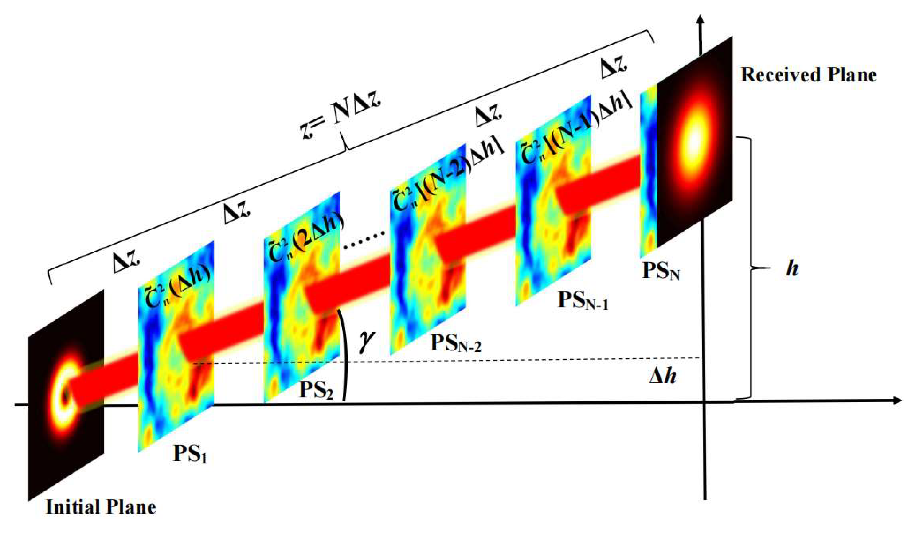
In addition, it is well known that the random phase screen (RPS) is an important method for simulating a beam propagating in atmospheric turbulence. Thus, we also use the RPS to simulate the propagation behaviors of a partially coherent LGVV beam in turbulence along a slant path. The core idea of the RPS is to regard the beam propagation process in atmospheric turbulence as two independent and simultaneous processes: vacuum propagation and phase modulation of an atmospheric turbulence medium [9,10,11,12]. Therefore, we can use a series of phase screens (PSs) spaced at Δz to replace the continuous random medium on the propagation path. A beam on the source plane passes through these PSs in turn to simulate the turbulence modulation effect and finally reaches the receive surface.

The simulation process can be characterized by [9,10,11,12]:

$$E_i\left(x,y;z_i\right)=F^{-1}\left\{F\left\{E_{i-1}\left(x,y;z_{i-1}\right)\exp \left[i\varphi \left(x,y;z_i\right)\right]\right\}\exp \left[-\frac{i\Delta z}{2k}\left({\kappa }_x^2+{\kappa }_y^2\right)\right]\right\},$$

(22)

where z_i−1 and z_i represent the position of the (i − 1)-th and i-th PS, E_i−1 (x, y; z_i−1) and E_i (x, y; z_i) are the fully coherent light field on the (i − 1)-th and i-th PS, ϕ (x, y; z_i) denotes the phase distribution in the i-th PS and F and F⁻¹ denote the Fourier transform and inverse Fourier transform, respectively.

The simulation process of the RPS of a partially coherent LGVV beam propagating in inhomogeneous atmospheric turbulence is different from that of horizontal propagation [9,10,11,12]. The main differences are as follows: the inhomogeneous atmospheric turbulence power spectrum used to generate the turbulence phase screen by the power spectrum inversion method changes with increasing propagation distance. In this paper, a schematic diagram of the simulation of the propagation of a partially coherent LGVV beam in inhomogeneous atmospheric turbulence is shown in Figure 1. We synthesized the turbulent phase with turbulent information and extended the RPS to the PC beam field by combining the complex screen (CS) method and multi-phase screen method. In summary, the logical process of numerical simulation of PC beams in atmospheric turbulence is described as follows. (1) Synthesize the corresponding turbulence PS and fix it on the propagation path. (2) Use J₁ CSs to synthesize a PC beam, and the electric field of each frame passes through the above PS fixed on the propagation path separately. It should be especially pointed out that the PS is variable. (3) The average value of the light intensity of J₁ frames on the receiving plane is a frame PC beam after propagating the atmospheric turbulence along the slant path. (4) Cycle steps (1)–(3) J₂ times to obtain the J₂ frame results of a PC beam through inhomogeneous atmospheric turbulence and use the J₂ frame results to analyze and calculate the statistical characteristics of PC beams through atmospheric turbulence along the slant path. J₁ and J₂ denote the number of CS and PS changes, respectively [9,10,11,12].

Next, we present some numerical examples to study the evolution behavior of the average intensity of a partially coherent LGVV beam propagating in inhomogeneous atmospheric turbulence. To facilitate this comparison, we fix some calculation parameters as follows: α = 3.4, λ = 632.8 nm, w₀ = 10 mm, δ₀ = 20 mm, L₀ = 100 m and l₀ = 10 mm. In the simulation of beam propagation, the distance between each two PSs is Δz = 50 m, and the number of data acquisition samples is set to 512 × 512. We take J₁ = 200, that is, one frame of instantaneous intensity of a partially coherent beam propagating through inhomogeneous atmospheric turbulence is simulated by the average intensity over 200 cycles. And the conversion times of PS are J₂ = 200, i.e., 200 frames of instantaneous light intensity of a partially coherent LGVV beam in inhomogeneous atmospheric turbulence are collected at the receiving plane, and the average of these 200 frames of instantaneous intensity is the final average intensity of a partially coherent LGVV beam through inhomogeneous atmospheric turbulence.

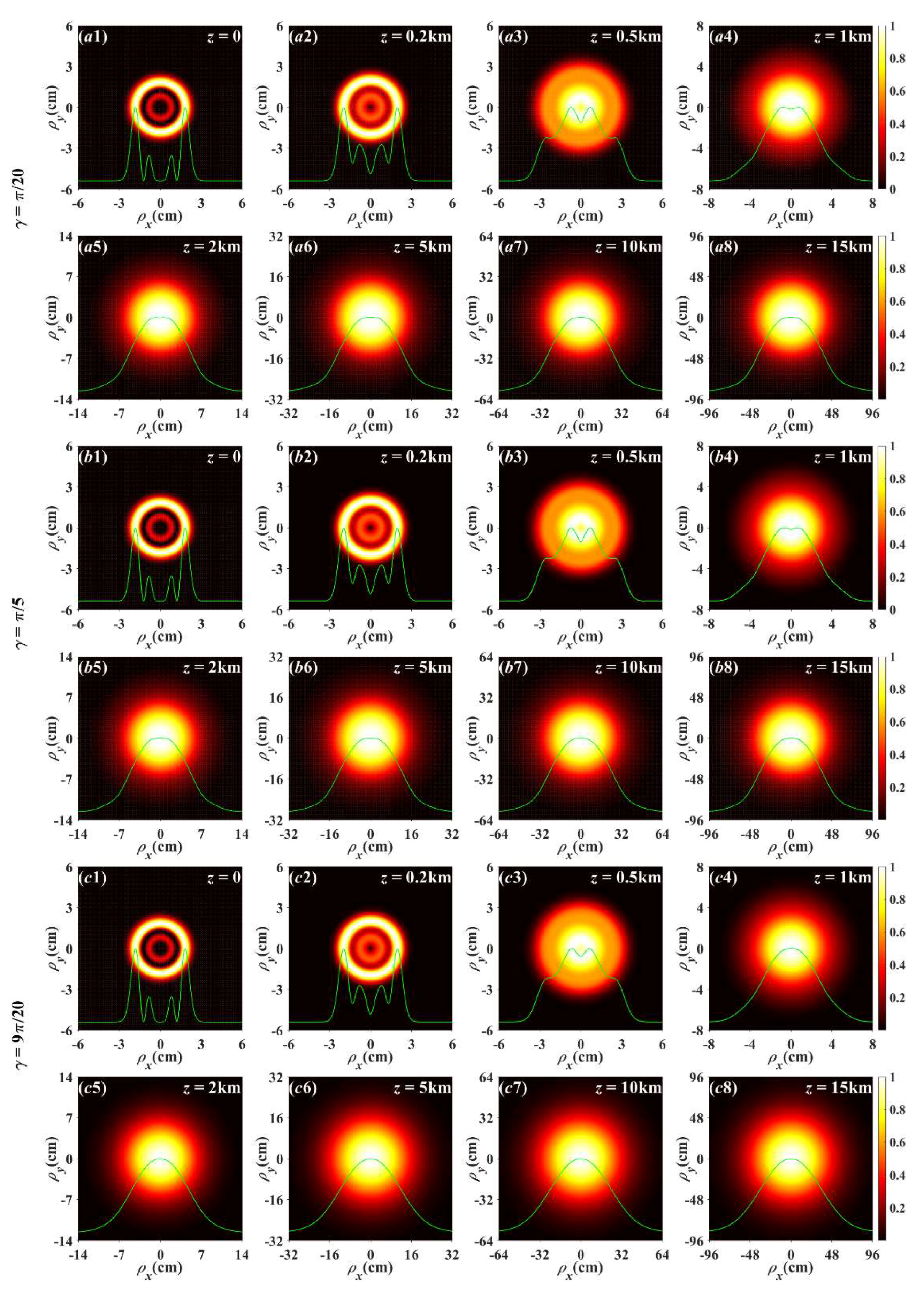
In Figure 2, we calculate the distribution of the normalized average intensity of a partially coherent LGVV beam with m = 2 and n = 1 through inhomogeneous atmospheric turbulence with different zenith angles at different propagation distances. It can be clearly found from Figure 2 that the beam profile on the initial plane is distributed in concentric rings [see Figure 2(a1,b1,c1)], and the intensity of the outer ring is higher than that of the inner ring. With the increase in the propagation distance, the dark spots and dark rings in the beam profile gradually decrease [see Figure 2(a2,b2,c2)], the central light intensity increases continuously, and the beam finally converts into a Gaussian-like beam distribution in the far field. We also find that a partially coherent LGVV beam will evolve into a Gaussian-like beam when it propagates 5 km from where the beam is emitted at the zenith angle of π/20 [see Figure 2(a6–a8)]. However, this evolution decreases to 2 km and 1 km for the zenith angles of π/5 [see Figure 2(b5–b8)] and 9π/20 [see Figure 2(c4–c8)], respectively. It also shows that the evolution behavior of a partially coherent LGVV beam in inhomogeneous atmospheric turbulence is greatly affected by the zenith angle. The larger the zenith angle is, the faster the beam evolves into a Gaussian-like beam [see Figure 2(c1–c8)] because the intensity of inhomogeneous atmospheric turbulence decreases as altitude increases. For the same propagation distance, the smaller the zenith angle is, the higher the propagation height above the ground of the beam is. The beam can quickly propagate into a weak atmospheric turbulence region, and the beam will be less affected by the cumulative influence of inhomogeneous atmospheric turbulence. In addition, we present some interesting physical phenomena in Figure 2. For different zenith angles (or inhomogeneous turbulence intensities), when a partially coherent LGVV beam propagates over short distances (z < 0.5 km), the evolution characteristics of the beam are almost independent of the turbulence intensity, and free-space diffraction plays a dominant role in the evolution of the beam. However, for long-distance propagation of a partially LGVV beam in atmospheric turbulence (z > 5 km), the effect of atmospheric turbulence on the phase structure of the emitted beam is greater with the increase in the zenith angle due to the cumulative effect of turbulence, which will accelerate the degradation of a partially coherent LGVV beam to a Gaussian-like distribution.

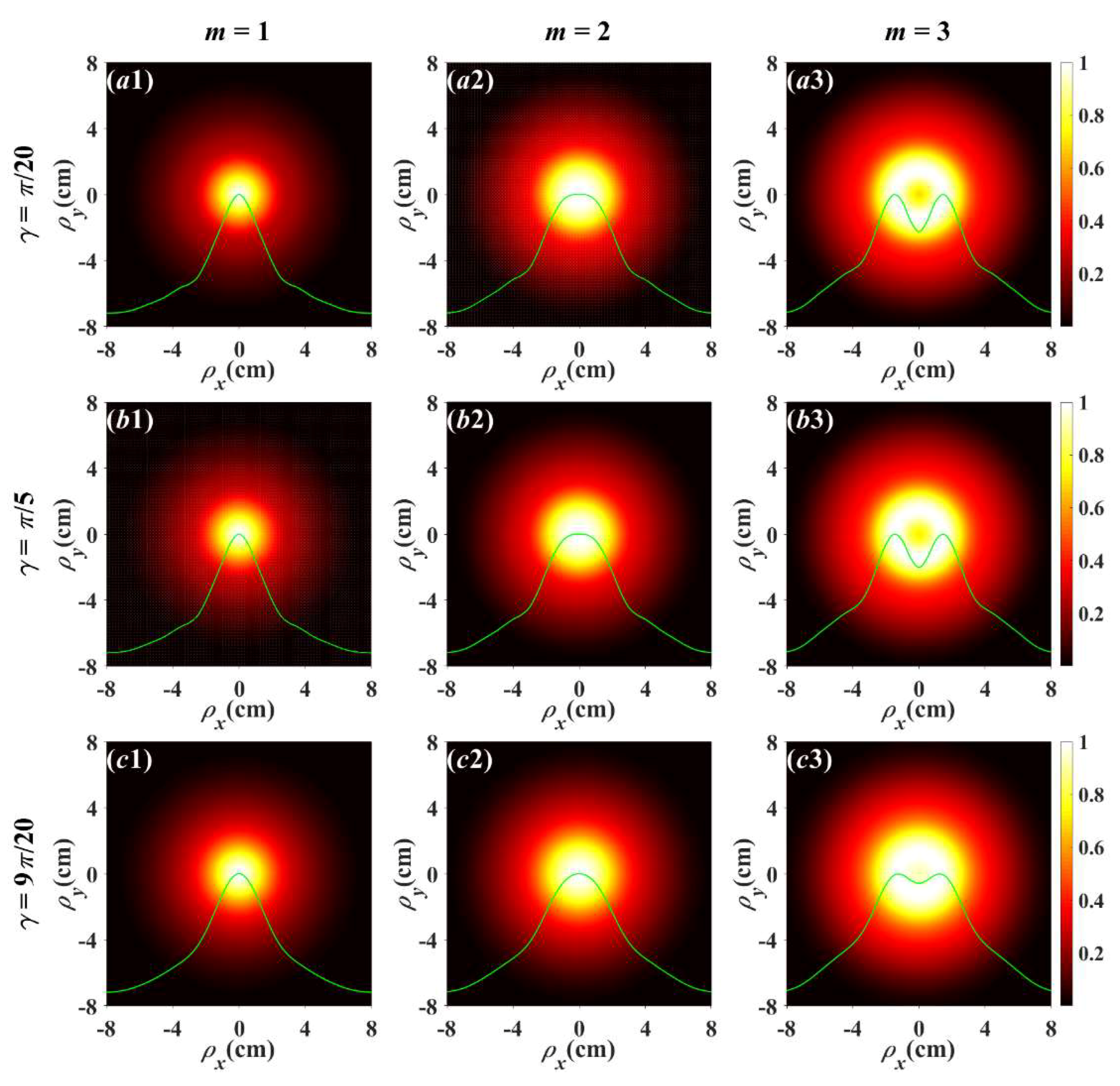
Figure 3 displays the normalized average intensity distribution of a partially coherent LGVV beam with different topological charge m through inhomogeneous atmospheric turbulence with different zenith angles at a propagation distance of z = 1 km. One can see that a partially coherent LGVV beam with a large m has a larger light spot. And under the same propagation distance, the larger the topological charge m is, the smaller the degree of hollowness (DOH) of the beam and the slower the beam degenerates into a Gaussian-like beam (in this paper, DOH is defined as the ratio of central light intensity to maximum light intensity). 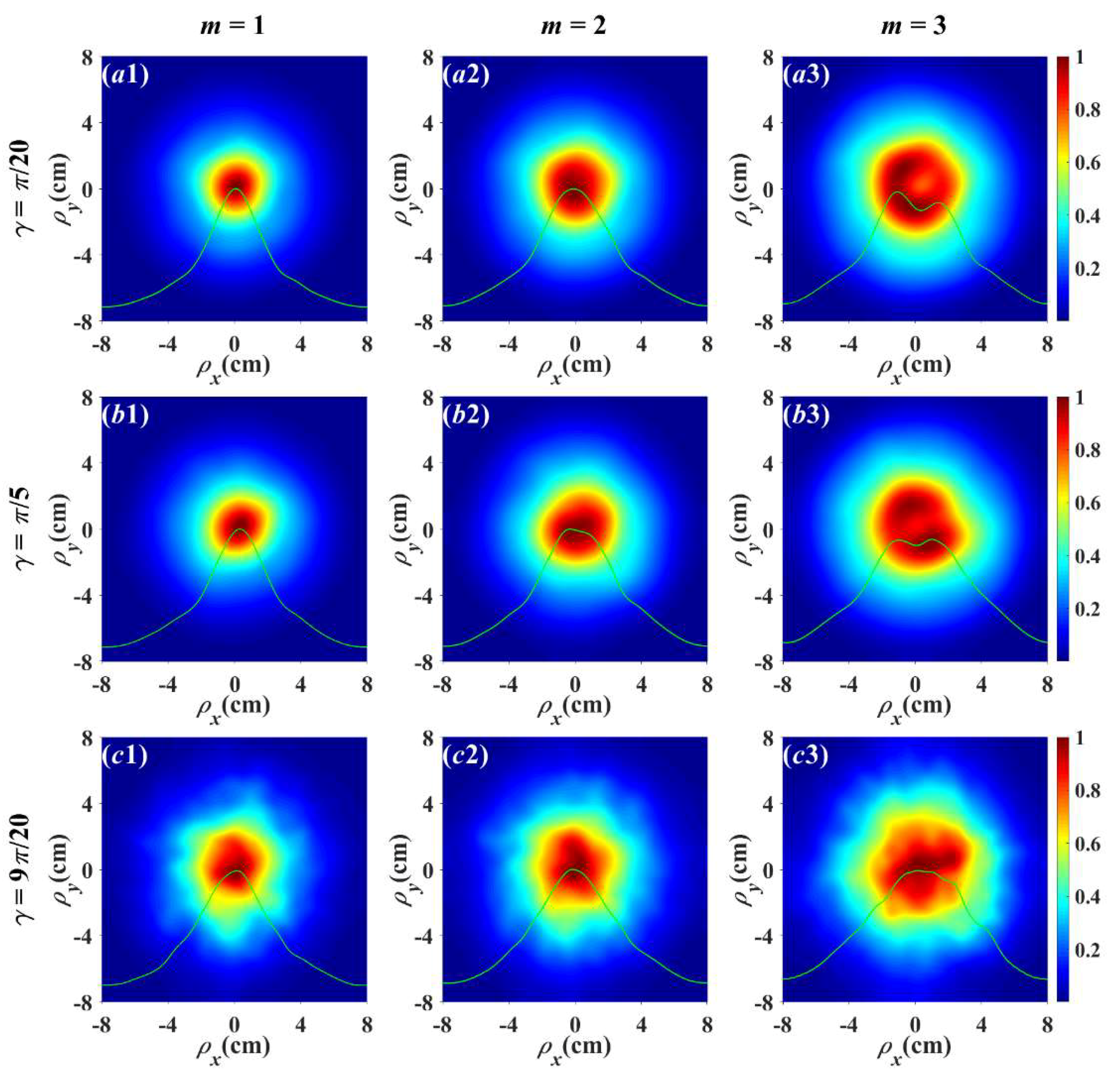This indicates that a partially coherent LGVV beam with a large m has a stronger ability to resist atmospheric turbulence. In order to confirm the theory model, the RPS method is used to simulate the propagation characteristics of a partially coherent LGVV beam in turbulence along a slant path, and the simulation results are shown in Figure 4. The calculated parameters in Figure 4 are the same as those in Figure 3. One can easily observe that the simulation results agree well with the theory, which indicates that our simulation model is valid and that the theoretical results are correct. Now, we explain the reasons for the physical phenomena in Figure 3 and Figure 4. As is well known, the orbital angular momentum of partially coherent vortex beams [9,10,11,25,33] can be given by mħ, and the larger the topological charge m is, the greater the orbital angular momentum. The smaller the influence of turbulence on the propagation of a partially coherent LGVV beam in atmospheric turbulence is, the stronger the ability to maintain a dark hollow shape. In Figure 4, the accuracy of the physical image is related to the number and interval Δz of phase screens.

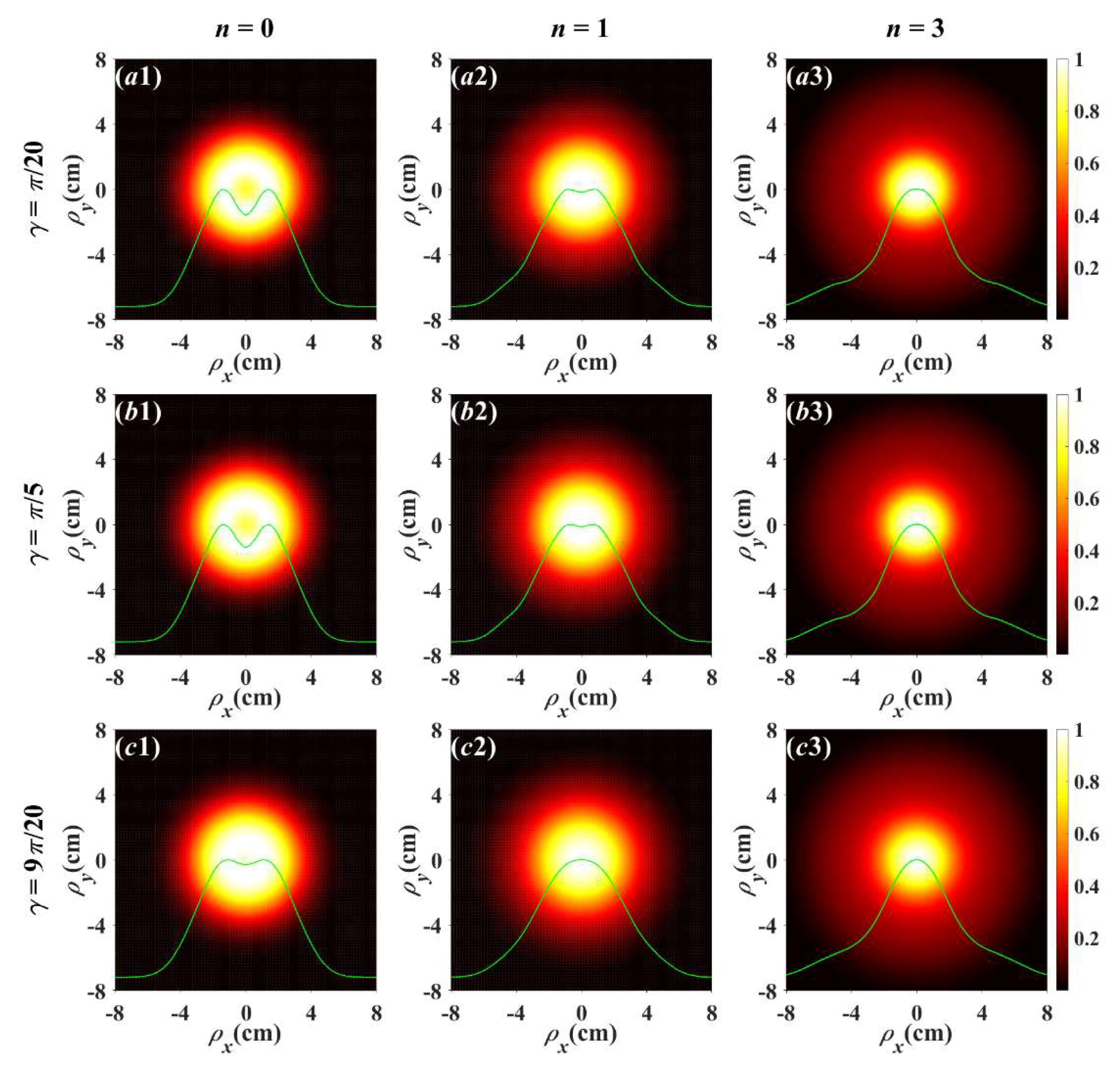
Further, to investigate the effect of radial index n on beam evolution behavior, in Figure 5, we show the distribution of the normalized average intensity of a partially coherent LGVV beam with different n through inhomogeneous atmospheric turbulence with different zenith angles at a propagation distance of z = 1 km. It can be found from Figure 5 that the influence of radial index n is quite different with topological charge m. It demonstrates that the larger n of a partially coherent LGVV beam is, the larger the DOH of the beam in inhomogeneous atmospheric turbulence, and the easier the beam tends to be the Gaussian-like distribution. 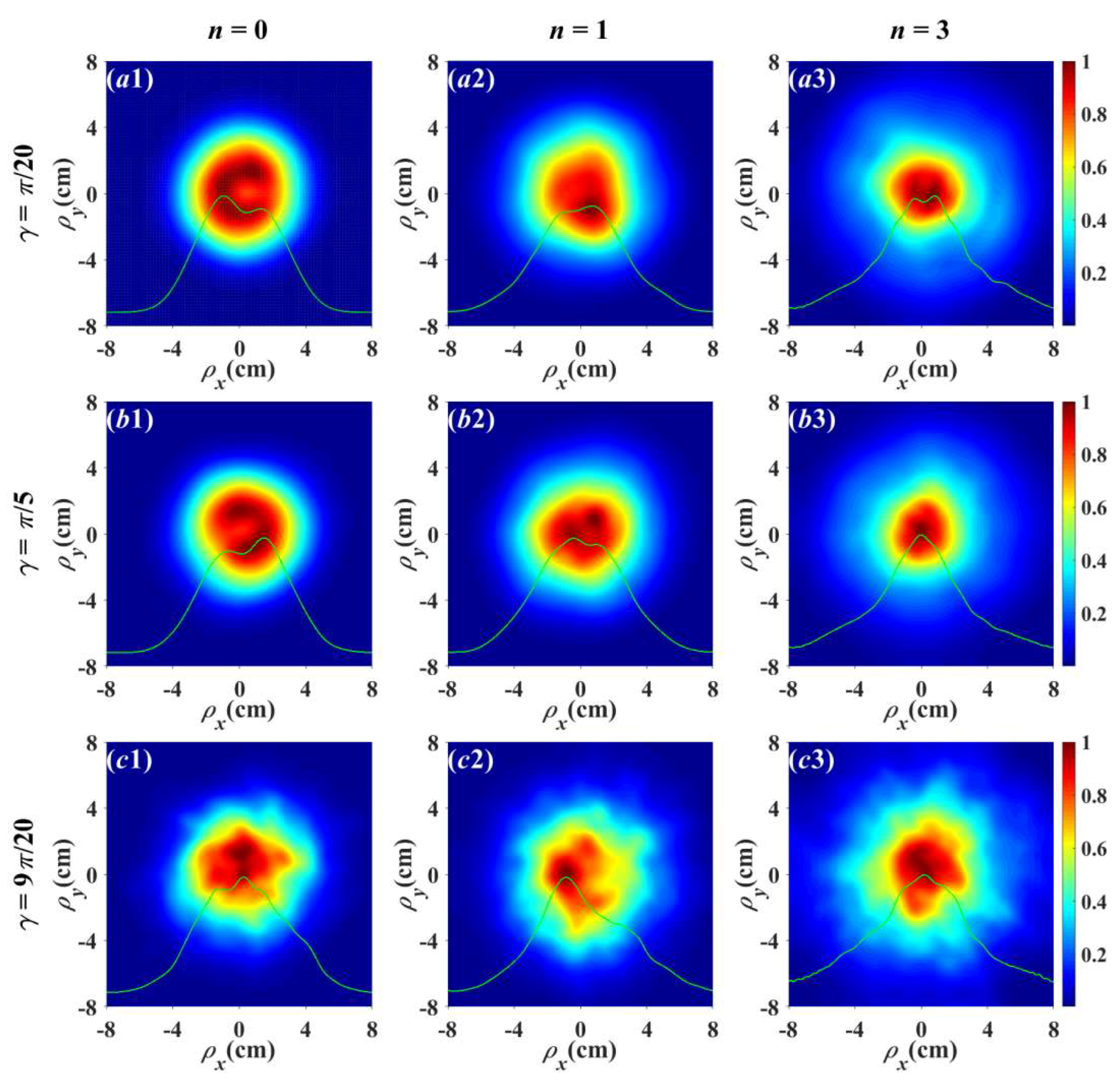This indicates that a partially coherent LGVV beam with a small radial index n has a stronger ability to resist atmospheric turbulence. Similarly, we also simulate the theoretical results shown in Figure 5, and the results are shown in Figure 6. The calculated parameters in Figure 6 are the same as those in Figure 5. We also find that Figure 6 is in good agreement with Figure 5. Now, we explain the reasons for the physical phenomena in Figure 5 and Figure 6. As is well known, the radial index n of partially coherent higher-order Laguerre–Gaussian vortex beams [10,30] will determine the dark rings. The larger n of the beam is, the more dark rings there are, and inhomogeneous atmospheric turbulence will cause an interaction between them; therefore, the DOH of the beam in inhomogeneous atmospheric turbulence will become large. In Figure 6, the accuracy of the physical image is also related to the number and interval of phase screens.

4. Conclusions

We have studied the propagation properties of a partially coherent LGVV beam in inhomogeneous atmospheric turbulence. Analytical formulae for the elements of a cross-spectral density matrix of a partially coherent LGVV beam propagating in turbulence are derived with the help of the extended Huygens–Fresnel principle. Numerical results indicate that the normalized initial profile with the concentric dark rings of a partially coherent LGVV beam gradually evolves into a Gaussian-like beam profile in turbulence. We also find that a partially coherent LGVV beam will evolve into a Gaussian-like beam when it propagates 5 km from where the beam is emitted at a zenith angle of π/20 [see Figure 2(a6–a8)]. However, this distance is reduced to 2 km and 1 km for zenith angles of π/5 [see Figure 2(b5–b8)] and 9π/20 [see Figure 2(c4–c8)], respectively. The reason is that the effect of atmospheric turbulence on the phase structure of the emitted beam is greater with the increase in the zenith angle due to the cumulative effect of turbulence, which will accelerate the degradation of a partially coherent LGVV beam to a Gaussian-like distribution.

Furthermore, under the same propagation distance of z = 1 km, the larger the topological charge m of a partially coherent LGVV beam is, the smaller the DOH of the beam and the slower the beam degenerates into a Gaussian-like beam. And the larger the radial index n of a partially coherent LGVV beam is, the larger the DOH of the beam in atmospheric turbulence along a slant path and the easier the beam tends to be a Gaussian-like beam distribution. Therefore, a partially coherent LGVV beam with large topological charge m and small radial index n has a stronger ability to resist atmospheric turbulence. In order to verify our numerical results, we combined the complex screen method and multi-phase screen method to simulate the propagation of a partially coherent LGVV beam in inhomogeneous atmospheric turbulence. It has been demonstrated that the simulation results are in good agreement with theoretical predictions. The reason is that a partially coherent LGVV beam with large topological charge m has a large orbital angular momentum. It is generally believed that our findings may have potential applications in free-space optical communications.

References

1. Andrews, L.C.; Phillips, R.L.; Crabbs, R. Propagation of a Gaussian-beam wave in general anisotropic turbulence. Proc. SPIE 2014, 9224, 922402. [Google Scholar]
2. Ricklin, J.C.; Davidson, F.M. Atmospheric turbulence effects on a partially coherent Gaussian beam: Implication for free-space laser communication. J. Opt. Soc. Am. A 2002, 19, 1794–1802. [Google Scholar] [CrossRef] [PubMed]
3. Shirai, T.; Dogariu, A.; Wolf, E. Mode analysis of spreading of partially coherent beams propagating through atmospheric turbulence. J. Opt. Soc. Am. A 2003, 20, 1094–1102. [Google Scholar] [CrossRef]
4. Yao, M.; Toselli, I.; Korotkova, O. Propagation of electromagnetic stochastic beams in anisotropic turbulence. Opt. Express 2014, 22, 31608–31619. [Google Scholar] [CrossRef]
5. Dong, Y.; He, J.; Li, S.; Zhang, X.; Jin, G. The propagation characteristics of the conical hollow beams in the turbulent atmosphere. Opt. Laser Technol. 2016, 82, 28–33. [Google Scholar]
6. Wang, J.; Zhu, S.; Wang, H.; Cai, Y.; Li, Z. Second-order statistics of a radially polarized cosine-Gaussian correlated Schell-model beam in anisotropic turbulence. Opt. Express 2016, 24, 11626–11639. [Google Scholar] [CrossRef] [PubMed]
7. Cheng, M.; Guo, L.; Li, J.; Yan, X.; Dong, K.; You, Y. Average intensity and spreading of a radially polarized multi-Gaussian Schell-model beam in anisotropic turbulence. J. Quant. Spectrosc. Radiat. Transf. 2018, 218, 12–20. [Google Scholar] [CrossRef]
8. Zhang, H.; Zhao, L.; Gao, Y.; Cai, Y.; Yuan, Y. Scintillation mitigation via the cross phase of the Gaussian Schell-model beam in a turbulent atmosphere. Opt. Express 2023, 31, 30615–30626. [Google Scholar] [CrossRef]
9. Yu, J.; Huang, Y.; Wang, F.; Liu, X.; Gbur, G.; Cai, Y. Scintillation properties of a partially coherent vector beam with vortex phase in turbulent atmosphere. Opt. Express 2019, 27, 26676–26688. [Google Scholar] [CrossRef]
10. Zhao, L.; Xu, Y.; Dan, Y. Evolution properties of partially coherent radially polarized Laguerre-Gaussian vortex beams in an anisotropic turbulent atmosphere. Opt. Express 2021, 29, 34986–35002. [Google Scholar] [CrossRef]
11. Xu, Q.; Zhao, L.; Xu, Y. Propagation properties of partially coherent radially and azimuthally polarized vortex beams in turbulent atmosphere. Optik 2022, 265, 169542. [Google Scholar] [CrossRef]
12. Yong, K.; Tang, S.; Yang, X.; Zhang, R. Propagation characteristics of a ring Airy vortex beam in slant atmospheric turbulence. J. Opt. Soc. Am. B 2021, 38, 1510–1517. [Google Scholar] [CrossRef]
13. Zhao, L.; Wang, J.; Guo, M.; Xu, X.; Qian, X.; Zhu, W.; Li, J. Steady-state thermal blooming effect of vortex beam propagation through the atmosphere. Opt. Laser Technol. 2021, 139, 106982. [Google Scholar] [CrossRef]
14. Zhang, B.; Huang, H.; Xie, C.; Zhu, S.; Li, Z. Twisted rectangular Laguerre-Gaussian correlated sources in anisotropic turbulent atmosphere. Opt. Commun. 2020, 459, 125004. [Google Scholar] [CrossRef]
15. Yan, Z.; Xu, Y.; Lin, S.; Chang, H.; Zhu, X.; Cai, Y.; Yu, J. Enhancing fiber-coupling efficiency of beam-to-fiber links in turbulence by spatial non-uniform coherence engineering. Opt. Express 2023, 31, 25680–25690. [Google Scholar] [CrossRef]
16. Allen, L.; Beijersbergen, M.; Spreeuw, R.; Woerdman, J. Orbital angular momentum of light and the transformation of Laguerre-Gaussian laser modes. Phys. Rev. A 1992, 45, 8185–8189. [Google Scholar] [CrossRef]
17. Grier, D. A revolution in optical manipulation. Nature 2003, 424, 810–816. [Google Scholar] [CrossRef]
18. MacDonald, M.P.; Paterson, L.; Volke-Sepulveda, K.; Arlt, J.; Sibbett, W.; Dholakia, K. Creation and manipulation of three-dimensional optically trapped structures. Science 2002, 296, 1101–1103. [Google Scholar] [CrossRef]
19. Melo, B.; Brandão, I.; da, B.S.P.; Rodrigues, R.; Khoury, A.; Guerreiro, T. Optical trapping in a dark focus. Phys. Rev. Appl. 2020, 14, 034069. [Google Scholar] [CrossRef]
20. Pu, J.; Zhao, K.; Zhou, Q.; Li, F. The study on the broadband thrust spectrum of propeller in anisotropic and inhomogeneous turbulence. Ocean Eng. 2022, 258, 111572. [Google Scholar] [CrossRef]
21. Chen, H.; Ji, X.; Li, X.; Wang, T.; Zhao, Q.; Zhang, H. Energy focusability of annular beams propagating through atmospheric turbulence along a slanted path. Opt. Laser Technol. 2015, 71, 22–28. [Google Scholar] [CrossRef]
22. Tan, W.; Huang, X.; Nan, S.; Bai, Y.; Fu, X. Ghost imaging through inhomogeneous turbulent atmosphere along an uplink path and a downlink path. OSA Contin. 2020, 3, 387075. [Google Scholar] [CrossRef]
23. Rogachevskii, I.; Kleeorin, N.; Zilitinkevich, S. Energy- and flux-budget theory for surface layers in atmospheric convective turbulence. Phys. Fluids 2022, 34, 116602. [Google Scholar] [CrossRef]
24. Chen, H.; Ji, X.; Ji, G.; Zhang, H. Scintillation characteristics of annular beams propagating through atmospheric turbulence along a slanted path. J. Opt. 2015, 17, 085605. [Google Scholar] [CrossRef]
25. Huang, K.; Xu, Y.; Cao, J.; Li, Y. Propagation characteristics of partially-coherent radially-polarized vortex beams through non-Kolmogorov turbulence along a slant path. J. Russ. Laser Res. 2023, 44, 110–120. [Google Scholar] [CrossRef]
26. Li, Y.; Li, L.; Guo, Y.; Zhang, H.; Fu, S.; Gao, C.; Yin, C. Atmospheric turbulence forecasting using two-stage variational mode decomposition and autoregression towards free-space optical data-transmission link. Front. Phys. 2022, 10, 970025. [Google Scholar] [CrossRef]
27. Wang, F.; Cai, Y.; Korotkova, O. Partially coherent standard and elegant Laguerre-Gaussian beams of all orders. Opt. Express 2009, 17, 22366–22379. [Google Scholar] [CrossRef]
28. Sidoro, K.; Luis, R. Relations between Hermite and Laguerre Gaussian modes. IEEE J. Quantum Electron. 1993, 29, 2563–2567. [Google Scholar]
29. Benzehoua, H.; Belafhal, A. Spectral properties of pulsed Laguerre higher-order cosh-Gaussian beam propagating through the turbulent atmosphere. Optics Commun. 2023, 541, 129492. [Google Scholar] [CrossRef]
30. Ma, Z.; Pan, Y.; Dou, J.; Zhao, J.; Li, B.; Hu, Y. Statistical properties of partially coherent higher-order Laguerre-Gaussian power-exponent phase vortex beams. Photonics 2023, 10, 461. [Google Scholar] [CrossRef]
31. Dan, Y.; Zhang, B.; Pan, P. Propagation of partially coherent flat-topped beams through a turbulent atmosphere. J. Opt. Soc. Am. A 2008, 25, 2223–2231. [Google Scholar] [CrossRef] [PubMed]
32. Liu, L.; Liu, Y.; Chang, H.; Huang, J.; Zhu, X.; Cai, Y.; Yu, J. Second-order statistics of self-splitting structured beams in oceanic turbulence. Photonics 2023, 10, 339. [Google Scholar] [CrossRef]
33. Peng, X.; Liu, L.; Yu, J.; Liu, X.; Cai, Y.; Baykal, Y.; Li, W. Propagation of a radially polarized twisted Gaussian Schell-model beam in turbulent atmosphere. J. Opt. 2016, 18, 125601. [Google Scholar] [CrossRef]
34. Wu, Z.; Feng, Z.; Ye, S.; Song, B.; Wei, R.; Yu, C. Beam properties of a partially coherent beam propagating horizontally in atmospheric turbulence. Photonics 2023, 10, 477. [Google Scholar] [CrossRef]
35. Huang, Y.; Wang, F.; Gao, Z.; Zhang, B. Propagation properties of partially coherent electromagnetic hyperbolic-sine-Gaussian vortex beams through non-Kolmogorov turbulence. Opt. Express 2015, 23, 1088–1102. [Google Scholar] [CrossRef]
Figure 1. Schematic diagram of the RPS method to simulate the propagation of a beam in inhomogeneous atmospheric turbulence.
Photonics 10 01189 g001
Figure 2. Normalized average intensity distribution and cross line of a partially coherent LGVV beam in inhomogeneous atmospheric turbulence with different zenith angles at different propagation distances; m = 2, n = 1. (a1a8): γ = π/20, (b1b8): γ = π/5, (c1–c8): γ = 9π/20.
Photonics 10 01189 g002
Figure 3. Normalized average intensity distribution and cross line of a partially coherent LGVV beam with different m in inhomogeneous atmospheric turbulence with different zenith angles at a propagation distance of z = 1 km; n = 2. (a1a3): γ = π/20, (b1b3): γ = π/5, (c1c3): γ = 9π/20.
Photonics 10 01189 g003
Figure 4. Simulation of the normalized average intensity and cross line of a partially coherent LGVV beam with different m in inhomogeneous atmospheric turbulence with different zenith angles at a propagation distance z = 1 km; n = 2. (a1a3): γ = π/20, (b1b3): γ = π/5, (c1c3): γ = 9π/20.
Photonics 10 01189 g004
Figure 5. Normalized average intensity distribution and cross line of a partially coherent LGVV beam with different n in inhomogeneous atmospheric turbulence with different zenith angles at a propagation distance of z = 1 km; m = 2. (a1a3): γ = π/20, (b1b3): γ = π/5, (c1c3): γ = 9π/20.
Photonics 10 01189 g005
Figure 6. Simulation of the normalized average intensity distribution and cross line of a partially coherent LGVV beam with different n in inhomogeneous atmospheric turbulence with different zenith angles at a propagation distance of z = 1 km; m = 2. (a1a3): γ = π/20, (b1b3): γ = π/5, (c1c3): γ = 9π/20.
Photonics 10 01189 g006
Disclaimer/Publisher’s Note: The statements, opinions and data contained in all publications are solely those of the individual author(s) and contributor(s) and not of MDPI and/or the editor(s). MDPI and/or the editor(s) disclaim responsibility for any injury to people or property resulting from any ideas, methods, instructions or products referred to in the content.