Bessel–Gauss Beams of Arbitrary Integer Order: Propagation Profile, Coherence Properties, and Quality Factor

Abstract

We present a novel approach to generate Bessel–Gauss modes of arbitrary integer order and well-defined optical angular momentum in a gradient index medium of transverse parabolic profile. The propagation and coherence properties, as well as the quality factor, are studied using algebraic techniques that are widely used in quantum mechanics. It is found that imposing the well-defined optical angular momentum condition, the Lie group $SU(1,1)$ comes to light as a characteristic symmetry of the Bessel–Gauss beams.

1. Introduction

Orbital angular momentum of light—more specifically, the orbital angular momentum about the axis of propagation [1]—has remained a lively and growing research topic over the last 30 years (see, for example, [1,2,3]). The paper that gave rise to this activity [4] communicated the idea that laser beams could carry orbital angular momentum and that this momentum would have measurable effects in the laboratory. Very early, the observation of angular momentum transfer from vortex beams to absorptive particles was reported [5], and the orbital angular momentum of light went from assumption to reality, forever changing the way we understand light. This fact arouses immediate interest in the study of the subject [6,7,8,9], specifically in the description, production, and detection of modes with well-defined orbital angular momentum [10,11,12,13,14,15,16,17]. This property of light is also known as optical angular momentum and goes by the acronym OAM (although there is no universal agreement on what the ‘O’ stands for [1], as it can mean both orbital and optical).

OAM beams find natural applications in optical communications [18] and the transfer of information [19], but are also useful in the quantum domain since OAM can be entangled [20]. Their ability to induce mechanical torque in absorptive systems makes them a critical ingredient in optical micro-manipulation, micro-machining, and optical tweezers [21].

Notably, the focusing and collimating properties of parabolic media allow propagation of vortex beams [16,22,23,24,25]. Indeed, the modal delay in the multiplexing of signals is greatly reduced using parabolic optical fibers [26] since they tolerate more than two modes with the same propagation constant (effective refractive index).

Among the most studied vortex beams, the Laguerre-Gauss, Bessel, and Bessel–Gauss modes stand out because their mathematical structure is well known, with which relatively simple theoretical models of their behavior are built, and because their practical realization seems viable in the laboratory [4,7,27,28,29,30,31,32,33,34].

Mathematically, Laguerre-Gauss modes constitute an orthonormal set that is very convenient to span the entire space of paraxial modes. There exist diverse techniques for their production in practice, including spiral plates, computer-generated diffractive gratings, mode converters, and spatial light modulators, among others [2].

Bessel modes, on the other hand, are non-diffractive and self-healing beams that preserve their transversal structure and reconstruct themselves after passing an obstacle in propagation events. In particular, the zero-order Bessel mode was found to be a solution of the Helmholtz equation in free space [28]. Indeed, it is a continuous superposition of plane waves for which the wave numbers form a cone around the optical axis. The non-diffraction phenomenon arises because the wave vectors have the same longitudinal component, so the plane wave components undergo the same phase shift, and identical intensity distributions are produced as the beam propagates along the optical axis.

However, the Bessel modes are not square-integrable, so their production would require an infinite amount of energy in practice. This limitation has been faced with the production of light beams whose intensity distribution acquires the Bessel profile in a finite circular area but which vanishes elsewhere in the transverse plane [29]. These beams retain some of the most important propagation properties that characterize Bessel beams, at least within a finite distance in the longitudinal direction. For example, they self-replicate by paraxial transformations that can be generated by either free-space propagation, thin lensing, parabolic media, or pure magnifiers [35]. In any case, although the production of Bessel beams can be described analytically, their experimental realization is far from simple.

Looking for analytical alternatives to the Bessel modes, it has already been proposed that the field amplitude profile can be factorized as a Bessel function and a Gaussian envelope. The Fresnel diffraction integral then led to the zero-order Bessel–Gauss mode in the paraxial approximation [30], a result verified in the laboratory by means of laser cavities [36]. On the other hand, within a bidirectional travel plane wave scheme, Bessel–Gauss modes of arbitrary integer order can be studied in terms of the exact solutions of the wave equation [37]. They can also be constructed as superpositions of Gaussian modes [30]. In the laboratory, ring arrays of Gaussian beams with wave vectors forming a cylinder or a cone around the propagation axis produce modified and generalized Bessel–Gauss modes, respectively [31]. Due to their non-diffractive properties, the Bessel–Gauss modes allow the design of secure communication protocols [38,39] and are more resilient than the Laguerre-Gauss modes under high-level turbulence conditions [40].

In this work, we study Bessel–Gauss modes of arbitrary integer order with well-defined OAM, propagating in a gradient index medium with a parabolic inhomogeneity in the transverse direction. Our approach is algebraic and translates notions that are quite natural in quantum mechanics to the field of optics.

The most striking feature of our approach is to find that not only the profile and the way the BG modes propagate along the z-axis but also their quality is determined by the underlying symmetry of well-defined OAM, which is linked to the Lie group $SU(1,1)$.

In Section 2, we analyze the paraxial equation for transverse parabolic media. We show that the well-defined angular momentum condition naturally leads to the solution space being interconnected by the generators of the $su(1,1)$ Lie algebra. Section 3 is addressed to show that the BG modes are generalized $su(1,1)$ coherent states and explore their coherence properties and quality factors in algebraic terms. A discussion of our results is given in Section 4.

At the end of the paper, we add an appendix with detailed calculations where it is shown that the subspaces of well-defined OAM are irreducible representation spaces for the Lie algebra $su(1,1)$.

2. Paraxial Wave Equation for Parabolic Media

The paraxial wave equation

$$\left[-\frac{1}{2k_0^2{n}_0}\left(\frac{{\partial }^2}{\partial x^2}+\frac{{\partial }^2}{\partial y^2}\right)+n_0\frac{{\mathsf{\Omega }}^2}{2}{r}^2\right]U=\frac{i}{k_0}\frac{\partial }{\partial z}U,{\mathsf{\Omega }}^2{r}^2\ll 1,$$

(1)

describes the z-propagation of electromagnetic waves through weakly inhomogeneous media with refractive index $n^2\left(r\right)=n_0^2\left(1-{\mathsf{\Omega }}^2{r}^2\right)$ [16,24,41,42]. The quantities $n_0\ge 1$ and $\mathsf{\Omega }\ge 0$ represent the refractive index at the optical axis and the strength of the medium inhomogeneity, respectively. In turn, $r\equiv \parallel \mathit{r}\parallel =\sqrt{x^2+y^2}$ denotes the norm of the position-vector $\mathit{r}\in {\mathbb{R}}^2$, which is transverse to the propagation axis. From now on we write $\mathit{r}$ in the polar form, with $\rho \ge 0$ and $\theta \in [-\pi ,\pi )$.

Equation (1) holds if one assumes that the electric field is of the form $\mathit{E}(\mathit{r},z)={\mathit{E}}_{\mathbf{0}}{e}^{i(k_0{n}_{0}z-\omega t)}U(\mathit{r},z)$, with ${\mathit{E}}_{\mathbf{0}}$ the field polarization, $k_0=\frac{\omega }{c}$ the wave number in free space, and $\omega =2\pi \nu$ the angular frequency. For $\mathsf{\Omega }\ne 0$, the complex amplitude $U(\mathit{r},z)$ represents a field mode that is guided within the inhomogeneous medium $n^2\left(r\right)$. The limit $\mathsf{\Omega }\to 0$ leads to the homogeneous case $n^2\left(r\right)=n_0^2$. At such a limit, the Rayleigh range $z_R=\frac{1}{2}{k}_0{n}_0{w}_0^2$ usually denotes the distance from the focal plane ($z=z_0$) over which a Gaussian beam increases its cross-sectional area by a factor of two. In this work, we follow [16,42] and set $\mathsf{\Omega }{z}_R=1$ to consider guided modes with constant beam width $w_0$.

2.1. Space of Solutions (Stationary and Guided LG Modes)

It may be shown [16] that the functions

$$U_{\ell }^p(\mathit{r},z)=\frac{e^{i\ell \theta }}{\sqrt{2\pi }}exp\left[-i\left(\frac{z-z_0}{z_R}\right){\beta }_{|\ell |}^p\right]{\mathsf{\Phi }}_{|\ell |}^p\left(\rho \right),\ell \in \mathbb{Z},p=0,1,2,\dots ,$$

(2)

are square-integrable solutions of the paraxial wave Equation (1) for $\mathsf{\Omega }{z}_R=1$, where

$${\beta }_{|\ell |}^p=|\ell |+2p+1$$

(3)

stands for the propagation constant, and

$${\mathsf{\Phi }}_{|\ell |}^p\left(\rho \right)=\frac{2{(-1)}^p}{w_0}\sqrt{\frac{\mathsf{\Gamma }(p+1)}{\mathsf{\Gamma }\left(\right|\ell |+p+1)}}{\left[\frac{\sqrt{2}\rho }{w_0}\right]}^{|\ell |}{L}_p^{\left(\right|\ell \left|\right)}\left(\frac{2{\rho }^2}{w_0^2}\right)exp\left(-\frac{{\rho }^2}{w_0^2}\right)$$

(4)

is the mode amplitude. In the above expressions, $z_0$ defines the origin of the longitudinal coordinate, $L_n^{\left(\alpha \right)}\left(x\right)$ is the associated Laguerre polynomial of degree n and order $\alpha$ [43], and $w_0$ stands for the (constant) beam width.

The mode amplitude (4) is defined on the plane transverse to the propagation direction as a function of the polar radial coordinate $\rho$ and is weighted by the Gaussian distribution of standard deviation $\sigma =w_0/\sqrt{2}$, i.e., ${\mathsf{\Phi }}_{|\ell |}^p\left(\rho \right)$ represents the electric field amplitude of a stationary Laguerre-Gauss mode.

The longitudinal and polar phases appearing in Equation (2) supply dynamical properties to the solutions $U_{\ell }^p(\mathit{r},z)$; they refer to the propagation of the beam and the helicity of the mode, respectively. The propagation occurs in the direction in which the variable z increases. In turn, the orientation of the helicity is based on the polar phase increments: if these are counterclockwise, the helicity is right-handed. Otherwise (clockwise), it is left-handed. The former is characterized by $\ell >0$, and the latter by $\ell <0$. Modes with null orbital angular momentum ($\ell =0$) do not exhibit helicity.

Please note that the helically phased modes $U_{\ell }^p$ and $U_{-\ell }^p$ have the same amplitude and longitudinal phase since neither the function (4) nor the propagation constant (3) depend on $sgn(\ell )$.

From now on, the functions $U_{\ell }^p(\mathit{r},z)$ introduced in (2) will be referred to as guided Laguerre-Gauss modes (LG modes for short).

In applications where a Gaussian distribution is the desired profile, the beam propagation factor ${\mathcal{M}}^2$ (also called beam quality factor) is the most important feature describing the quality of the beam. It was introduced to characterize laser beams by comparing their beam parameter product (waist-radius × divergence) with that of a Gaussian beam [44,45]. As a parameter, it determines how close a given light field is to an ideal Gaussian beam [46,47].

For the LG modes (2), the factor ${\mathcal{M}}^2$ coincides with the propagation constant (3). The lowest value ${\beta }_0^0=1$ refers to the fundamental LG mode $U_0^0$, which represents a Gaussian beam. Higher-order modes $U_{\ell }^p$ may be grouped according to the nonnegative integer $n=|\ell |+2p$, for which we write ${\beta }_{|\ell |}^p\equiv {\beta }_{\left(n\right)}=n+1$. In this form, ℓ and p can be combined in $n+1$ different ways to get the same value

$${\beta }_{|\ell |}^p=\underset{n+1 terms}{\underbrace{{\beta }_{|-n|}^0={\beta }_{|-n+2|}^1=\cdots ={\beta }_{n-2}^1={\beta }_n^0}}\equiv {\beta }_{\left(n\right)}=n+1;n=|\ell |+2p=fixed.$$

That is, there are $n+1$ modes $U_{\ell }^p$ with exactly the same propagation constant ${\beta }_{|\ell |}^p={\beta }_{\left(n\right)}$. In other words, ${\beta }_{|\ell |}^p$ is $(n+1)$-fold degenerate for $n=|\ell |+2p=fixed$.

For practical purposes, one may identify the ensemble $\left\{{\beta }_{\left(n\right)}\right\}$ with the energy eigenvalues of a two-dimensional quantum harmonic oscillator (2D quantum oscillator for short), see Figure 1.

The set $\left\{U_{\ell }^p\right\}$ is orthonormal and compete according to the inner product

$${\int }_{-\pi }^{\pi }{\int }_0^{\infty }{U}_{\ell }^{p\ast }(\mathit{r},z)U_l^q(\mathit{r},z)\rho d\rho d\theta ={\delta }_{\ell ,l}{\delta }_{p,q},$$

(5)

where $u^{\ast }$ stands for the complex-conjugate of $u\in \mathbb{C}$. Hence, the LG modes (2) form an orthonormal basis for the solution space $\mathcal{H}$ of the paraxial wave Equation (1). We formally write

$$\mathcal{H}=span\{U_{\ell }^p(\mathit{r},z);\ell \in \mathbb{Z},p=0,1,2,\dots \}.$$

Given (5), each of the functions $U_{\ell }^p(\mathit{r},z)$ represents a collimated beam that carries finite transverse optical power as it propagates along the z-axis [16].

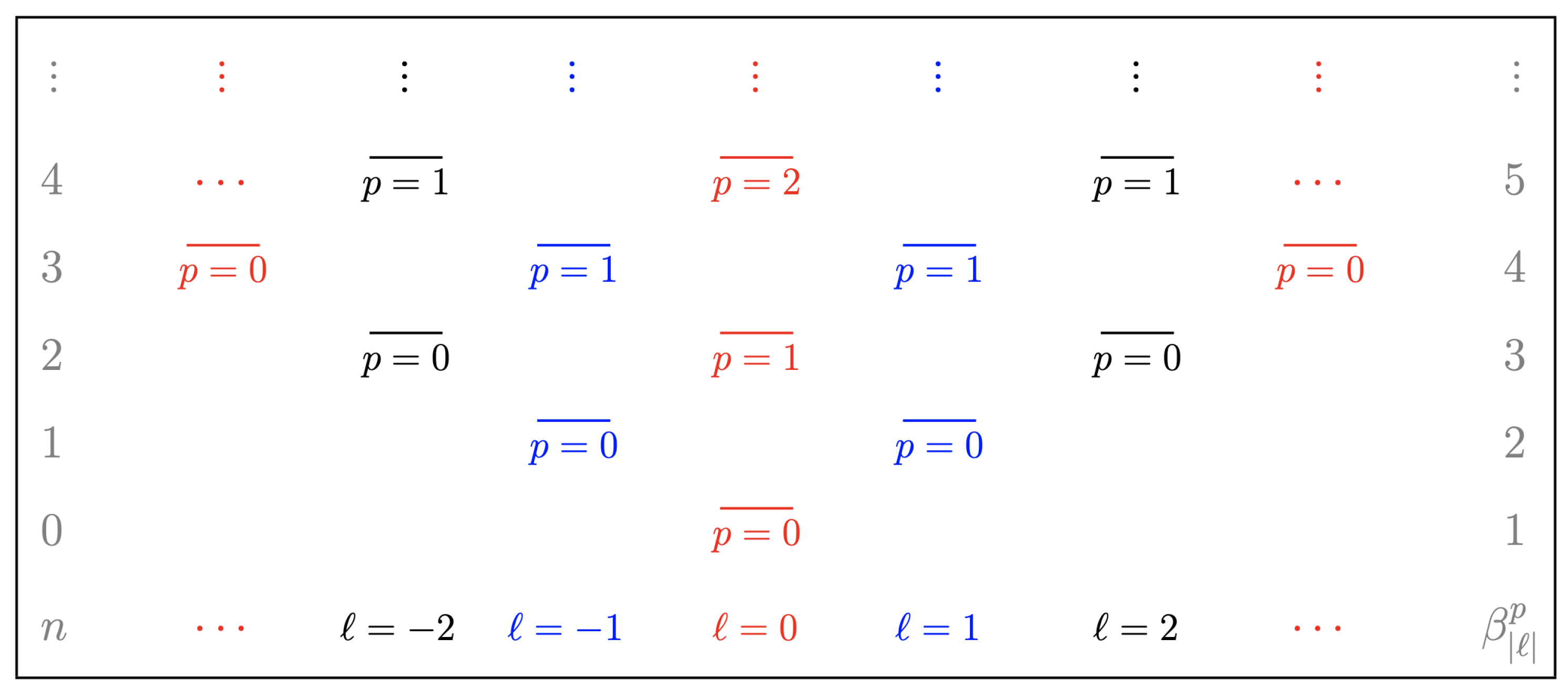
2.2. Subspaces with a Well-Defined Optical Angular Momentum

It is convenient to classify the LG modes into hierarchies of well-defined optical angular momentum $\ell \in \mathbb{Z}$, which are defined as the solution subspaces

$$\mathcal{H}\supset {\mathcal{H}}_{\ell }=span\{U_{\ell }^p(\mathit{r},z);\ell =fixed,p=0,1,2,\dots \},\ell \in \mathbb{Z}.$$

Hierarchies ${\mathcal{H}}_{\ell }$ are infinite-dimensional and satisfy $\mathcal{H}={⨁}_{\ell }{\mathcal{H}}_{\ell }$. They are characterized by a denumerable set of propagation constants ${\beta }_{|\ell |}^p$ that are equidistant, with steps of two units ${\beta }_{|\ell |}^{p+1}-{\beta }_{|\ell |}^p=2$, see Figure 1.

Considering that LG modes are helically phased, we may write ${\mathcal{H}}^{-}={⨁}_{\ell <0}{\mathcal{H}}_{\ell }$, ${\mathcal{H}}^{+}={⨁}_{\ell >0}{\mathcal{H}}_{\ell }$, and ${\mathcal{H}}^0={\mathcal{H}}_{\ell =0}$ for the solution subspaces with clockwise, counterclockwise and null helicity, respectively. Then, the entire space of solutions is also written as $\mathcal{H}={\mathcal{H}}^{-}⨁{\mathcal{H}}^0⨁{\mathcal{H}}^{+}$.

Hereafter we work on the elements of the hierarchy ${\mathcal{H}}_{\ell }$. Our interest is addressed to manipulate the coherence properties of electromagnetic modes with a well-defined optical angular momentum. With this in mind, the association of the ensemble $\left\{{\beta }_{|\ell |}^p\right\}$ with the energy spectrum of the 2D quantum oscillator is very useful.

By translating the algebraic structure of contemporary quantum mechanics to study the optical system we are dealing with, we have a beautiful tool at hand for designing LG-mode superpositions on demand. In particular, we look for the optimization of the coherence properties of wave packets with a well-defined optical angular moment.

We have successfully carried out this translation; details are given in Appendix A. There, a series of ladder operators is constructed such that a certain LG mode $U_{\ell }^p(\mathit{r},z)$ is connected to another $U_l^q(\mathit{r},z)$, where p and q, and ℓ and l, are different in general.

The most striking feature of the algebraic formalism developed in Appendix A is that the symmetry underlying the hierarchy ${\mathcal{H}}_{\ell }$ is associated with the $su(1,1)$ Lie algebra:

$$[{\mathcal{L}}_{\ell }^{-},{\mathcal{L}}_{\ell }^{+}]=2{\mathcal{L}}_{\ell },[{\mathcal{L}}_{\ell },{\mathcal{L}}_{\ell }^{\pm }]=\pm {\mathcal{L}}_{\ell }^{\pm },$$

the generators of which are defined as follows:

$${\mathcal{L}}_{\ell }^{-}=e^{i2\frac{(z-z_0)}{z_R}}\frac{1}{\sqrt{\rho }}{L}_{\ell }^{-}\sqrt{\rho },{\mathcal{L}}_{\ell }^{+}=e^{-i2\frac{(z-z_0)}{z_R}}\frac{1}{\sqrt{\rho }}{L}_{\ell }^{+}\sqrt{\rho },{\mathcal{L}}_{\ell }=\frac{1}{\sqrt{\rho }}{L}_{\ell }\sqrt{\rho }.$$

Here, $L_{\ell }^{\pm }$ and $L_{\ell }$ are the second-order differential operators

$$L_{\ell }^{\pm }=\frac{1}{2}{\left(\frac{w_0}{2}\right)}^2\left[\frac{{\partial }^2}{\partial {\rho }^2}-\frac{(\ell +\frac{1}{2})(\ell -\frac{1}{2})}{{\rho }^2}\right]\mp \frac{1}{2}\rho \frac{\partial }{\partial \rho }+\frac{1}{2}\frac{{\rho }^2}{w_0^2}\mp \frac{1}{4},$$

and

$$L_{\ell }=\frac{1}{2}{\left(\frac{w_0}{2}\right)}^2\left[-\frac{{\partial }^2}{\partial {\rho }^2}+\frac{(\ell +\frac{1}{2})(\ell -\frac{1}{2})}{{\rho }^2}\right]+\frac{1}{2}\frac{{\rho }^2}{w_0^2}.$$

Note that $L_{\ell }$ coincides with the radial part of the energy observable of a 2D quantum oscillator in position representation.

The LG mode $U_{\ell }^p(\mathit{r},z)$ is an eigenfunction of ${\mathcal{L}}_{\ell }$ with eigenvalue ${\lambda }_p=\frac{1}{2}{\beta }_{|\ell |}^p=\frac{|\ell |}{2}+p+\frac{1}{2}$ (to simplify the notation, we have made the dependence of ${\lambda }_p$ on ℓ implicit). The ensemble $\left\{{\lambda }_p\right\}$ mimics the energy spectrum (shifted by $\frac{|\ell |}{2}$) of the one-dimensional harmonic oscillator in quantum mechanics, see

Table 1. The Laguerre-Gauss modes $U_{\ell }^p(\mathit{r},z)$ are eigenfunctions of ${\mathcal{L}}_{\ell }$ with eigenvalue ${\lambda }_p=\frac{|\ell |}{2}+p+\frac{1}{2}$ (it is shown only the information for the first three values of p and $|\ell |$). The number p of nodes admitted by the mode along the $\rho$-axis defines both ${\lambda }_p$ and the propagation constant ${\beta }_{|\ell |}^p=2{\lambda }_p$, and thus determines the way the mode propagates along the z-axis.

${\mathit{\lambda }}_{\mathit{p}}$	$\mathit{\ell }=0$	$\mathit{\ell }=\pm 1$	$\mathit{\ell }=\pm 2$	$\mathit{\ell }=\pm 3$
${\lambda }_0$	1/2	1	3/2	2
${\lambda }_1$	3/2	2	5/2	3
${\lambda }_2$	5/2	3	7/2	4
${\lambda }_3$	7/2	4	9/2	5

. In turn, ${\mathcal{L}}_{\ell }^{\pm }$ are ladder operators of the LG modes, i.e., the action of ${\mathcal{L}}_{\ell }^{\pm }$ on $U_{\ell }^p(\mathit{r},z)$ produces an eigenfunction of ${\mathcal{L}}_{\ell }$ with eigenvalue ${\lambda }_p\pm 1={\lambda }_{p\pm 1}$.

The nonnegative integer p corresponds to the number of nodes admitted by the LG mode along the $\rho$-axis, i.e., p refers to the behavior of the mode on the plane transverse to the propagation direction. Although the latter is stationary, the value of p defines the propagation constant (eigenvalue) ${\beta }_{|\ell |}^p=2{\lambda }_p$ since $\ell =const$ in ${\mathcal{H}}_{\ell }$ and thus determines the way the mode propagates along the z-axis. Therefore, it is appropriate to find a way to determine p in the basis elements of ${\mathcal{H}}_{\ell }$.

In Appendix A, we have introduced a differential operator ${\widehat{n}}_p$, called the harmonic-number (number for short), which acts on the transverse (stationary) part of the LG modes and returns the corresponding number of nodes, as requested. In this form, according to the number drawn by ${\widehat{n}}_p$, the eigenvalues (propagation constants) ${\lambda }_p=\frac{1}{2}{\beta }_{|\ell |}^p$ define the fundamental harmonic ($p=0$) as well as the higher harmonics ($p\ge 1$) in any superposition of LG modes. The role that ${\widehat{n}}_p$ plays in the description of light beams with well-defined optical angular momentum is of fundamental importance, as we are going to see.

3. Guided Bessel–Gauss Modes as Generalized Coherent States

Once we have incorporated the algebraic structure of quantum mechanics in the description of light beams with well-defined optical angular momentum, it is acceptable to translate some quantum mechanical concepts to the arena of electromagnetic waves. Of course, the latter are still defined by the Maxwell theory, regardless of the algebraic techniques used in their analysis, which seem more natural in quantum theory.

Of particular interest, the notion of coherence introduced by Glauber in quantum optics [48] is intrinsically algebraic, so it has been generalized to encompass systems other than light (for a recent review, see [49]).

In what follows, we adhere to the more general notion of a coherent state: it is a linear superposition that exhibits some specific properties that are determined by the ‘user’ based on the phenomenology under study or on theoretical arguments [49]. With this in mind, we look for superpositions of LG modes with a well-defined optical angular momentum.

According to Barut and Girardello [50], the normalized solution of the eigenvalue equation

$${\mathcal{L}}_{\ell }^{-}{V}_{\ell }(\mathit{r},z;\xi )=\xi V_{\ell }(\mathit{r},z;\xi ),\xi =\tau e^{-i\varphi },\tau \ge 0,\varphi \in [-\pi ,\pi ),$$

(6)

defines a coherent state for the Lie algebra we are dealing with.

To solve Equation (6), we first express $V_{\ell }(\mathit{r},z;\xi )$ in terms of the basis of ${\mathcal{H}}_{\ell }$,

$$V_{\ell }(\mathit{r},z;\xi )=\sum _{p=0}^{\infty }{c}_p{U}_{\ell }^p(\mathit{r},z),c_p\in \mathbb{C}.$$

The coefficients $c_p$ are defined by the action of the ladder operator ${\mathcal{L}}_{\ell }^{-}$ on the LG modes $U_{\ell }^p(\mathit{r},z)$, so the precise form of $V_{\ell }(\mathit{r},z;\xi )$ is directly associated with the symmetry underlying the hierarchy ${\mathcal{H}}_{\ell }$, which is characterized by the Lie algebra $su(1,1)$. The explicit calculation yields

$$V_{\ell }(\mathit{r},z;\xi )={\left[\frac{2{\tau }^{|\ell |}}{\pi w_0^2{I}_{|\ell |}\left(2\tau \right)}\right]}^{1/2}{\left[\frac{\sqrt{2}\rho }{w_0}\right]}^{|\ell |}{e}^{i\ell \theta }{e}^{-\frac{i}{z_R}\left(\right|\ell |+1)(z-z_0)}{e}^{-\frac{{\rho }^2}{w_0^2}}{\mathsf{\Lambda }}_{\ell }(\rho ,z,\xi ),$$

where $I_{\nu }$ stands for the modified Bessel function [43], and ${\mathsf{\Lambda }}_{\ell }(\rho ,z,\xi )$ is the superposition

$${\mathsf{\Lambda }}_{\ell }(\rho ,z,\xi )=\sum _{p=0}^{\infty }\frac{{\left(\tau e^{-i\varphi }{e}^{-i\frac{2}{z_r}(z-z_0)}{e}^{i\pi }\right)}^p}{\left(\right|\ell |+p)!}{L}_p^{\left(\right|\ell \left|\right)}\left(\frac{2{\rho }^2}{w_0^2}\right).$$

Further simplification is achieved using the series and connection formulas [43,51]

$$J_{\nu }\left(2\sqrt{uv}\right)e^v{\left(uv\right)}^{-\frac{\nu }{2}}=\sum _{k=0}^{\infty }\frac{v^k}{(k+\nu )!}{L}_k^{\left(\nu \right)}\left(u\right),J_{\nu }\left(u{e}^{\pm i\pi /2}\right)=e^{\pm i\nu \pi /2}{I}_{\nu }\left(u\right),$$

(7)

where $J_{\nu }$ denotes the Bessel function of the first kind. We finally write

$$\begin{array}{c}{V}_{\ell }(\mathit{r},z;\xi )=exp\left\{i\left[\ell \theta +\frac{|\ell |}{2}\varphi -\frac{(z-z_0)}{z_R}+\tau sin\left(\varphi +\frac{2}{z_R}(z-z_0)\right)\right]\right\}\\ \times {\left[\frac{2}{\pi w_0^2{I}_{|\ell |}\left(2\tau \right)}\right]}^{1/2}exp\left[-\frac{{\rho }^2}{w_0^2}-\tau cos\left(\varphi +\frac{2}{z_R}(z-z_0)\right)\right]\\ \times I_{|\ell |}\left(\frac{2\sqrt{2\tau }}{w_0}\rho e^{-\frac{i}{2}\varphi }{e}^{-\frac{i}{z_R}(z-z_0)}\right).\end{array}$$

(8)

Hereafter the functions (8) will be referred to as Bessel–Gauss coherent states (BG coherent states or BG modes for short). We also simplify notation by making $z_0=0$.

Next, we clarify the role played by the real and imaginary parts of the eigenvalue $\xi =\tau e^{-i\varphi }$ in the description of the BG modes.

• Fundamental Gaussian mode. Using the properties of the modified Bessel function $I_{\nu }$ [43,51] one has

  $$\underset{\xi \to 0}{lim}{V}_{\ell }(\mathit{r},z;\xi )=\left\{\begin{array}{cc}\sqrt{\frac{2}{\pi w_0^2}}exp\left(-i\frac{z}{z_R}\right)exp\left(-\frac{{\rho }^2}{w_0^2}\right),& \ell =0\\ 0,& \ell \ne 0\end{array}\right..$$

  (9)

That is, for $\xi =0$, there is only one regular solution to the Barut-Girardello Equation (6), given by the fundamental Gaussian mode $V_{\ell =0}(\mathit{r},z;0)=U_{\ell =0}^{p=0}(\mathit{r},z)$, which is a coherent state by definition.

• Modified Bessel and Bessel profiles. For $\xi \ne 0$ the functions $V_{\ell }(\mathit{r},z;\xi )$ consist of a modified Bessel function $I_{|\ell |}$ modulated by a Gaussian distribution of standard deviation $\sigma =w_0/\sqrt{2}$. The latter accelerates the radial decay of the beam. Depending on the eigenvalue-phase $\varphi$, the function $I_{|\ell |}$ is interchanged by $J_{|\ell |}$, and vice versa (the same occurs at specific points along the propagation axis, see details below).

For example, making $\varphi =0$, the profile of $V_{\ell }(\mathit{r},z;\tau )$ is determined by the modified Bessel function $I_{|\ell |}$ in (8). However, from the connection formula included in Equation (7), we see that $\varphi =-\pi$ replaces $I_{|\ell |}$ with the Bessel function $J_{|\ell |}$ in (8). Thus, we have

$$\begin{array}{c}{V}_{\ell }(\mathit{r},z;-\tau )={\left[\frac{2}{\pi w_0^2{I}_{|\ell |}\left(2\tau \right)}\right]}^{1/2}exp\left\{i\left[\ell \theta -\frac{z}{z_R}-\tau sin\left(\frac{2z}{z_R}\right)\right]\right\}\\ \times exp\left[-\frac{{\rho }^2}{w_0^2}+\tau cos\left(\frac{2z}{z_R}\right)\right]J_{|\ell |}\left(\frac{2\sqrt{2\tau }}{w_0}\rho e^{-i\frac{z}{z_R}}\right).\end{array}$$

(10)

This result shows that the phase $\varphi$ of the complex eigenvalue $\xi \ne 0$ characterizes the Bessel profile of our coherent states.

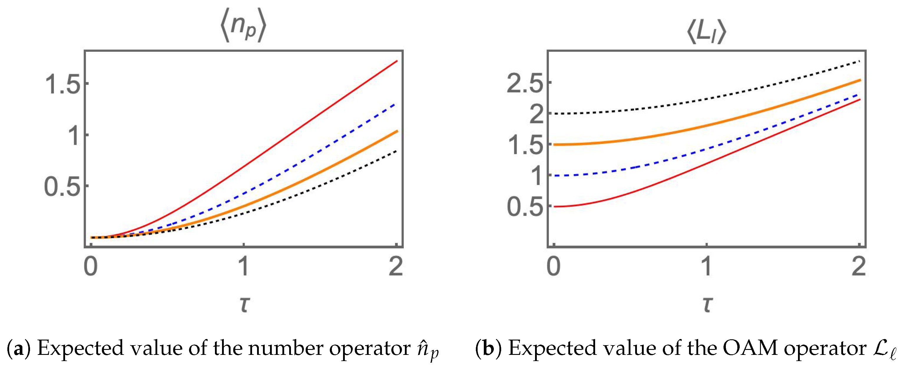
• Contribution of the p-th harmonic. The most likely eigenvalue ${\lambda }_p$ occurring in the superposition $V_{\ell }(\mathit{r},z;\xi )$ is determined by the expectation value $\langle {\mathcal{L}}_{\ell }\rangle =\langle {\widehat{n}}_p\rangle +\frac{1}{2}\left(\right|\ell |+1)$. The helicity parameter ℓ is fixed, so the relevant information is encoded in the expectation value of the number operator ${\widehat{n}}_p$. The straightforward calculation yields

  $$\langle {\widehat{n}}_p\rangle =\frac{\tau I_{|\ell |+1}\left(2\tau \right)}{I_{|\ell |}\left(2\tau \right)}.$$

  (11)
  Figure 2a shows the behavior of $\langle {\widehat{n}}_p\rangle$ as a function of $\left|\xi \right|=\tau$. In general, it can be seen that $\langle {\widehat{n}}_p\rangle$ decreases quadratically with $\tau <1$ but increases linearly with $\tau >1$. The latter is easily verified from the properties of the modified Bessel function $I_{\nu }$ [43], so one has

  $${\langle {\widehat{n}}_p\rangle }_{\tau \ll 1}\approx \left(\frac{1}{|\ell |+1}\right){\tau }^2,{\langle {\widehat{n}}_p\rangle }_{\tau \gg 1}\approx \tau .$$

  (12)

Figure 2. The quality of the Bessel–Gauss modes $V_{\ell }(\mathit{r},z;\xi )$ can be manipulated in terms of the parameter $\left|\xi \right|=\tau$. The harmonics $\langle {\widehat{n}}_p\rangle =p$ occur at smaller values of $\tau$ for smaller values of $|\ell |$ (a). The fundamental harmonic ($p=0$) is only permitted for $\ell =0$. Therefore, the lowest eigenvalue $\langle {\mathcal{L}}_{\ell }\rangle ={\lambda }_0=\frac{1}{2}\left(\right|\ell |+1)$ never occurs in higher BG modes (b). The BG modes are as close to the ideal Gaussian beam as the expected value $\langle {\mathcal{L}}_{\ell }\rangle$ is close to ${\lambda }_0$, which occurs in the vicinity of $\tau =0$. The color-code is as follows: $\ell =0$ (continuous, narrow-red), $\ell =1$ (dashed, blue), $\ell =2$ (continuous, wide-orange), and $\ell =3$ (dotted, black).

Figure 2. The quality of the Bessel–Gauss modes $V_{\ell }(\mathit{r},z;\xi )$ can be manipulated in terms of the parameter $\left|\xi \right|=\tau$. The harmonics $\langle {\widehat{n}}_p\rangle =p$ occur at smaller values of $\tau$ for smaller values of $|\ell |$ (a). The fundamental harmonic ($p=0$) is only permitted for $\ell =0$. Therefore, the lowest eigenvalue $\langle {\mathcal{L}}_{\ell }\rangle ={\lambda }_0=\frac{1}{2}\left(\right|\ell |+1)$ never occurs in higher BG modes (b). The BG modes are as close to the ideal Gaussian beam as the expected value $\langle {\mathcal{L}}_{\ell }\rangle$ is close to ${\lambda }_0$, which occurs in the vicinity of $\tau =0$. The color-code is as follows: $\ell =0$ (continuous, narrow-red), $\ell =1$ (dashed, blue), $\ell =2$ (continuous, wide-orange), and $\ell =3$ (dotted, black).

In Figure 2a, we see that the fundamental harmonic $\langle {\widehat{n}}_{p=0}\rangle =0$ occurs at $\tau =0$, which by necessity implies $\ell =0$, see Equation (9). The higher harmonics $\langle {\widehat{n}}_p\rangle =p\ge 1$ occur at smaller values of $\tau$ for smaller values of $|\ell |$.

On the other hand, Figure 2b shows that the higher eigenvalues $\langle {\mathcal{L}}_{\ell }\rangle ={\lambda }_p$, $p\ge 1$, occur at larger values of $\tau$ for larger values of $|\ell |$. Remarkably, with the exception of the fundamental BG mode, the lowest eigenvalue $\langle {\mathcal{L}}_{\ell }\rangle ={\lambda }_0$ never occurs in higher BG modes since $\langle {\widehat{n}}_{p=0}\rangle =0$ is not defined for $\ell \ne 0$.

The latter means that only the fundamental BG mode behaves like a Gaussian beam. In turn, the higher BG modes are as close to the ideal Gaussian beam as the expected value $\langle {\mathcal{L}}_{\ell }\rangle$ is close to ${\lambda }_0$ (see Table 1), which occurs in the vicinity of $\tau =0$.

Clearly, the modulus of the complex eigenvalue $\xi$ is responsible for the quality of the BG modes. By setting $\tau$ close to zero, we can make the BG modes as Gaussian as the limit $\tau \to 0$ allows.

The contribution of the p-th harmonic to the coherence of the BG mode $V_{\ell }(\mathit{r},z;\xi )$ is more easily visualized using the square modulus of the related coefficient

$$|c_p{(\ell ,\tau )|}^2=\frac{{\tau }^{|\ell |+2p}}{I_{|\ell |}\left(2\tau \right)\mathsf{\Gamma }(p+1)\mathsf{\Gamma }\left(\right|\ell |+p+1)}.$$

For small values of $\tau$, the above expression acquires the form

$$|c_p{(\ell ,\tau )|}^2\approx \frac{{\tau }^{2p}\mathsf{\Gamma }\left(\right|\ell |+1)}{\mathsf{\Gamma }(p+1)\mathsf{\Gamma }\left(\right|\ell |+p+1)}.$$

In the vicinity of $\tau =0$ one has ${\tau }^0>{\tau }^2>{\tau }^4>\cdots$. Therefore, the harmonics labeled with small p contribute more significantly to increasing the quality of the BG mode. This is illustrated in Figure 3. Clearly, $c_0$ provides the largest square modulus for $\tau \approx 0$, so the fundamental LG mode is dominant in any superposition intended to build high-quality BG modes. The contribution of the remaining harmonics can be treated as a disturbance (noise) that deviates the BG mode from the ideal Gaussian profile.

3.1. Variances and Standard Deviations

We now introduce the quadratures

$${\mathcal{L}}_{1;\ell }=\frac{{\mathcal{L}}_{\ell }^{+}+{\mathcal{L}}_{\ell }^{-}}{2},{\mathcal{L}}_{2;\ell }=\frac{{\mathcal{L}}_{\ell }^{+}-{\mathcal{L}}_{\ell }^{-}}{2i},$$

which are non-commuting variables $[{\mathcal{L}}_{1;\ell },{\mathcal{L}}_{2;\ell }]=-i{\mathcal{L}}_{\ell }$. Using the BG modes, the related variances are equally weighted:

$${\mu }_{{\mathcal{L}}_{1;\ell }}={\mu }_{{\mathcal{L}}_{2;\ell }}=\frac{1}{2}\langle {\mathcal{L}}_{\ell }\rangle .$$

As a consequence, the inequality

$${\sigma }_{{\mathcal{L}}_{1;\ell }}{\sigma }_{{\mathcal{L}}_{2;\ell }}\ge \frac{1}{2}\left|\langle [{\mathcal{L}}_{1;\ell },{\mathcal{L}}_{2;\ell }]\rangle \right|,$$

named after Robertson [52], is saturated.

The latter means that the average errors of ${\mathcal{L}}_{1;\ell }$ and ${\mathcal{L}}_{2;\ell }$ are not only the same but minimal (it is said that the BG modes are minimum uncertainty states). Then, it may not be possible to prepare a state with both distributions, ${\sigma }_{{\mathcal{L}}_{1;\ell }}$ and ${\sigma }_{{\mathcal{L}}_{2;\ell }}$, sharply concentrated around any concrete value [53]. Therefore, to characterize the BG modes $V_{\ell }(\mathit{r},z;\xi )$, we need to set up another uncertainty relationship, the one that holds for the appropriate observables.

In the formal operator description of paraxial wave optics, the canonical conjugate variables of transverse-position $\mathit{r}$ and transverse-propagation direction $\mathit{p}$ are treated as self-adjoint operators, see for example [54,55]. Using the BG modes, the mean value of such variables vanishes for the on-axis beams, $\langle \mathit{r}\rangle =\langle \mathit{p}\rangle =0$. Additionally, the straightforward calculation yields $\langle [\mathit{r},\mathit{p}]\rangle =\frac{2}{k_0}$, together with

$${\mu }_{\mathit{r}}=w_0^2\left[\langle {\mathcal{L}}_{\ell }\rangle +\tau cos\left(\frac{2z}{z_R}+\varphi \right)\right],{\mu }_{\mathit{p}}=\frac{4}{k_0^2{w}_0^2}\left[\langle {\mathcal{L}}_{\ell }\rangle -\tau cos\left(\frac{2z}{z_R}+\varphi \right)\right].$$

(13)

Therefore, the Robertson inequality for $\mathit{r}$ and $\mathit{p}$ gives

$${\sigma }_{\mathit{r}}{\sigma }_{\mathit{p}}=\frac{2}{k_0}{\left[{\langle {\mathcal{L}}_{\ell }\rangle }^2-{\tau }^2{cos}^2\left(\frac{2z}{z_R}+\varphi \right)\right]}^{1/2}\ge \frac{1}{k_0}.$$

(14)

If $\tau \ne 0$, the transverse-spreading ${\sigma }_{\mathit{r}}{\sigma }_{\mathit{p}}$ oscillates between two extreme values

$${\sigma }_{\mathit{r}}{\sigma }_{\mathit{p}}{|}_{max}=\frac{2}{k_0}\langle {\mathcal{L}}_{\ell }\rangle ,{\sigma }_{\mathit{r}}{\sigma }_{\mathit{p}}{|}_{min}=\frac{2}{k_0}\sqrt{{\langle {\mathcal{L}}_{\ell }\rangle }^2-{\tau }^2},$$

(15)

which are periodically attained at $z_n=\frac{1}{2}[(n+\frac{1}{2})\pi -\varphi ]z_R$ and $z_q=\frac{1}{2}(q\pi -\varphi )z_R$, respectively, with $n,q\in \mathbb{Z}$.

The above results exhibit the self-focusing and collimation properties of the BG modes and show that the corresponding beam is collimated.

By necessity, if $\tau =0$, then $\ell =0$. In such a case, the transverse-spreading ${\sigma }_{\mathit{r}}{\sigma }_{\mathit{p}}$ is constant and acquires the global minimum value

$${\sigma }_{\mathit{r}}{\sigma }_{\mathit{p}}{|}_{Gauss}=k_0^{-1},$$

(16)

so it saturates inequality (14). The latter because $V_{\ell =0}(\mathit{r},z;\xi =0)$ is the fundamental Gaussian mode $U_0^0(\mathit{r},z)$, see Equation (9).

Figure 4a shows a comparison between the extreme values (15) of the transverse-spreading ${\sigma }_{\mathit{r}}{\sigma }_{\mathit{p}}$, as a function of $\tau =\left|\xi \right|$, for $\ell =0,1,2,3$. The smaller $\tau$, the shorter the difference ${\sigma }_{\mathit{r}}{\sigma }_{\mathit{p}}{{|}_{max} - {\sigma }_{\mathit{r}}{\sigma }_{\mathit{p}}|}_{min}$, which confirms that the beam is better collimated for small values of $\tau$.

3.2. Beam Quality

We would like to emphasize that $\langle \mathit{r}\rangle =\langle \mathit{p}\rangle =0$ is just a necessary condition (but not sufficient) for $\mathit{r}$ and $\mathit{p}$ to fluctuate totally independently from another. Indeed, after Schrödinger [56] it is currently known that the Robertson inequality includes the skew Hermitian part $[\mathit{r},\mathit{p}]$ of the product $\mathit{rp}$, but it omits the complementary Hermitian part. In fact, taking into account the complete decomposition $\mathit{rp}=\frac{1}{2}\{\mathit{r},\mathit{p}\}+\frac{1}{2}[\mathit{r},\mathit{p}]$, with $\{·,·\}$ the anticommutator of the involved operators, we should follow Schrödinger, who proposed the more precise inequality

$$\sqrt{{\mu }_{\widehat{u}}{\mu }_{\widehat{v}}-{\left[\frac{1}{2}\langle \{\widehat{u},\widehat{v}\}\rangle -\langle \widehat{u}\rangle \langle \widehat{v}\rangle \right]}^2}\ge \frac{1}{2}\left|\langle [\widehat{u},\widehat{v}]\rangle \right|.$$

(17)

The term in square brackets under the square-root symbol is known as covariance and measures the joint variability of $\widehat{u}$ and $\widehat{v}$ when non-commutability is taken into account.

In addition to (13), for the present case one has $\langle \{\mathit{r},\mathit{p}\}\rangle =-\frac{4}{k_0}\tau sin(\frac{2z}{z_R}+\varphi )$. Then, the Schrödinger inequality (17) yields $\sqrt{{\langle {\mathcal{L}}_{\ell }\rangle }^2-{\tau }^2}\ge \frac{1}{2}$, i.e., considering the non-commutability of $\mathit{r}$ and $\mathit{p}$, the Robertson inequality (14) must be corrected to only compare ${\sigma }_{\mathit{r}}{\sigma }_{\mathit{p}}{|}_{min}$ with the lowest bound $k_0^{-1}$ (that is, with the transverse-spreading of an ideal Gaussian beam). Taking this conclusion into account, we introduce the function

$$M_{\ell }^2\left(\tau \right):=k_0{\sigma }_{\mathit{r}}{\sigma }_{\mathit{p}}{|}_{min}=k_0\sqrt{{\mu }_{\mathit{r}}{\mu }_{\mathit{p}}-\frac{1}{4}{\langle \{\mathit{r},\mathit{p}\}\rangle }^2}=2\sqrt{{\langle {\mathcal{L}}_{\ell }\rangle }^2-{\tau }^2},$$

(18)

which satisfies $M_{\ell }^2\left(\tau \right)\ge 1$, see Figure 4b. The lowest bound $M_0^2\left(0\right)=1$ corresponds to the fundamental Gaussian mode $V_{\ell =0}(\mathit{r},z;\xi =0)=U_0^0(\mathit{r},z)$.

The function (18) may be identified with the ${\mathcal{M}}^2$ factor of light signals [46,47], which is often used to specify the beam quality [44,45]: the higher the value of ${\mathcal{M}}^2$, the lower is the beam quality. By definition, the lowest value ${\mathcal{M}}^2=1$ is assigned to Gaussian beams, which are called diffraction-limited beams.

Indeed, the very last expression of (18) coincides with the ${\mathcal{M}}^2$ factor obtained in [32] for generic Bessel–Gauss beams. The authors of [32] develop a direct calculation of the second-order moments associated with the intensity distributions at the waist plane and in the far field, denoted ${\sigma }_0$ and ${\sigma }_{\infty }$ respectively, to write ${\mathcal{M}}^2=2\pi {\sigma }_0{\sigma }_{\infty }$. Here, we have simplified the derivation of such a result using algebraic techniques, with no cumbersome calculations involved.

Additionally, the penultimate expression of (18) is commonly used as a definition of the ${\mathcal{M}}^2$ factor when the first-order moments of the canonical variables vanish, as for the case of on-axis paraxial beams. But the calculation of moments is extremely difficult in general, so there are only a few examples where it has been possible [57,58]. It is then extremely interesting to provide either models allowing the calculation of higher-order moments or innovative approaches addressed to circumvent technical difficulties. However, it is notable that the intimate relation between the beam quality factor ${\mathcal{M}}^2$ and the Schrödinger inequality (17) is barely recognized in the literature. Remarkable exceptions are [59], where it is suggested a link between some invariant quantities and generalized uncertainty relations like the Schrödinger one, and [24], where the ${\mathcal{M}}^2$ factor of Hermite-Gauss modes is directly related to the Schrödinger inequality for $\mathit{r}$ and $\mathit{p}$.

In the present work, we have exploited the fact that the Schrödinger correction to the Robertson inequality (14) eliminates the sinusoidal z-dependence of the product ${\sigma }_{\mathit{r}}{\sigma }_{\mathit{p}}$, and considers only the minimal value ${\sigma }_{\mathit{r}}{\sigma }_{\mathit{p}}{|}_{min}$ to measure the joint variability of $\mathit{r}$ and $\mathit{p}$ when non-commutability is taken into account. It is then relevant to find that the $M_{\ell }^2$ factor (18) coincides with ${\sigma }_{\mathit{r}}{\sigma }_{\mathit{p}}{|}_{min}$.

For small values of $\tau$, the ${\mathcal{M}}^2$ factor behaves as follows

$${\left.M_{\ell }^2\left(\tau \right)\right|}_{\tau \ll 1}\approx \frac{2{\tau }^4}{{\left(\right|\ell |+1)}^3}+|\ell |+1.$$

(19)

At the very limit $\tau \to 0$, the lowest value $M_{\ell }^2(\tau =0)=|\ell |+1$ is only reached for $\ell =0$, i.e., the ideal Gaussian profile $M_{\ell =0}^2(\tau =0)=1$ occurs for the fundamental mode $V_{\ell =0}=U_{\ell =0}^{p=0}$ only, as we have already mentioned.

For $\ell \ne 0$, the quality of the BG mode obeys the rule $M_{\ell }^2\left(\tau \right)>|\ell |+1$. How close $M_{\ell }^2\left(\tau \right)$ is to its lower bound depends on how close $\tau$ is to zero.

However, keep in mind that the optical angular momentum $\ell \hslash$ spoils the beam quality: poor beam quality results for large $|\ell |$, no matter how small $\tau$ is.

Therefore, our previous conclusion is reinforced: the fundamental LG mode is dominant in wave packets, leading to high-quality BG modes. The remaining harmonics contribute by producing noise, so the BG mode deviates from the ideal Gaussian profile. The smaller the value of the mean $\langle {\widehat{n}}_p\rangle$, the better the quality of the BG mode. A high mean harmonic number means a very large factor $M_{\ell }^2$ for the BG beams.

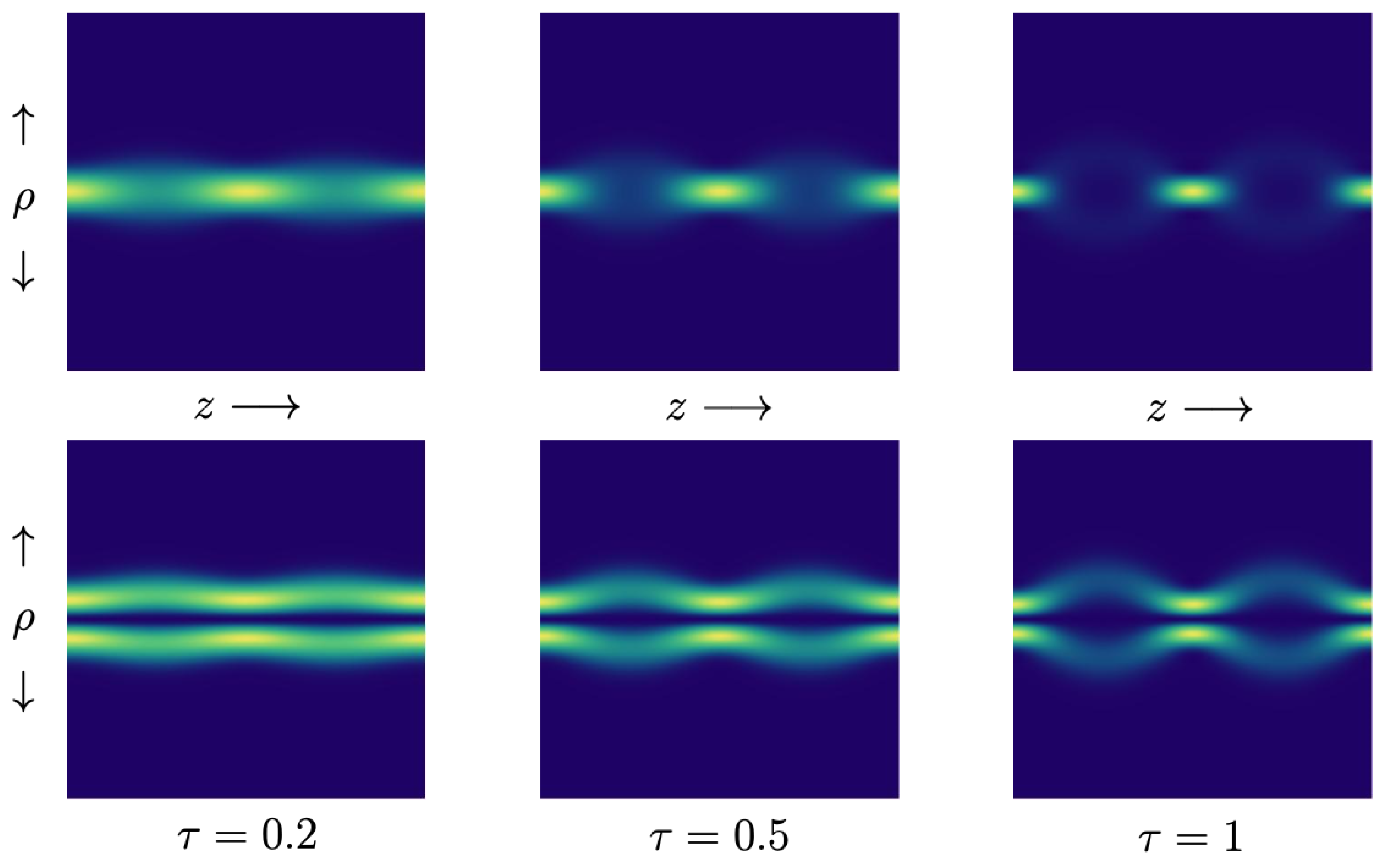
3.3. Propagation Properties

Please note that although the BG modes (8) are superpositions of LG modes with constant width, they exhibit self-focus since the propagation constants are commensurable, so their initial transversal profile is reproduced periodically along the propagation direction, see Figure 5.

The intensity $|V_{\ell }{(\mathit{r},z;\xi )|}^2$ is symmetrical with respect to rotations around the propagation axis and periodical in z with period $\pi z_R$ since $V_{\ell }(\mathit{r},z;\xi )$ is periodical in z with period $2\pi z_R$. For $\ell =0$ and any value of z, the intensity is different from zero at $\rho =0$, so it depicts a spot on the transverse plane. However, if $\ell \ne 0$, the intensity cancels at $\rho =0$ and is distributed in an annular way on the transverse plane for any value of z.

The maximum transverse-spreading of the beam is parameterized by $\left|\xi \right|=\tau$. On the other hand, for propagation along the z-axis, the following periodical identities are obeyed

$$\begin{array}{c}{V}_{\ell }(\mathit{r},2z_q;\xi )=V_{\ell }(\mathit{r},0;\xi ),|V_{\ell }(\mathit{r},z_q;\xi ){|}^2={\left|V_{\ell }(\mathit{r},0;\xi )\right|}^2,\\ V_{\ell }(\mathit{r},z_n;\xi )={(-1)}^{n\left(\right|\ell |+1)}{V}_{\ell }(\mathit{r},\frac{\pi }{2}{z}_R;\xi ),|V_{\ell }(\mathit{r},z_n;\xi ){|}^2={\left|V_{\ell }(\mathit{r},\frac{\pi }{2}{z}_R;\xi )\right|}^2,\end{array}$$

(20)

where

$$z_q=q\pi z_R,z_n=(n+\frac{1}{2})\pi z_R,q,n\in \mathbb{Z},$$

and

$$\begin{array}{c}{V}_{\ell }(\mathit{r},\frac{\pi }{2}{z}_R;\xi )={\left[\frac{2}{\pi w_0^2{I}_{|\ell |}\left(2\tau \right)}\right]}^{1/2}exp\left\{i\left[\ell \theta +\frac{|\ell |}{2}\varphi -\frac{\pi }{2}\left(\right|\ell |+1)-\tau sin\varphi \right]\right\}\\ \times exp\left[-\frac{{\rho }^2}{w_0^2}+\tau cos\varphi \right]J_{|\ell |}\left(\frac{2\sqrt{2\tau }}{w_0}\rho e^{-\frac{i}{2}\varphi }\right).\end{array}$$

(21)

Identities (20) mean that both the mode field and the cross-section change periodically as the beam propagates. Thus, there is a finite spread of the optical power that is reverted periodically at concrete points along the propagation axis.

In turn, function (21) reveals that the Bessel profile of the coherent states $V_{\ell }(\mathit{r},z;\xi )$ changes from $I_{|\ell |}$ to $J_{|\ell |}$ at the odd multiples of a quarter of the period $2\pi z_R$, no matter the value of the phase $\varphi$.

Next, we analyze the propagation properties of the BG coherent states $V_{\ell }(\mathit{r},z;\xi )$ for the real eigenvalue $\xi =-\tau$ ($\varphi =-\pi$) and the pure imaginary one $\xi =i$ ($\varphi =\frac{\pi }{2}$). The behavior for any other value of $\varphi$ is qualitatively equivalent to such cases.

3.3.1. Behavior for Real Eigenvalues

For $\xi =-\tau$, the functions $V_{\ell }(\mathit{r},z;-\tau )$ are defined in Equation (10). The choice $\xi =\tau$ gives rise to an expression quite similar to (10), but including the modified Bessel function $I_{|\ell |}$ instead of $J_{|\ell |}$. The qualitative behavior of $V_{\ell }(\mathit{r},z;\xi )$ is basically the same for either $\xi =-\tau$ or $\xi =\tau$. Hence, we consider $V_{\ell }(\mathit{r},z;-\tau )$ as representative of the BG coherent states (8) for $\xi \in \mathbb{R}$.

• Initial configuration and periodicity. Considering $z=0$ as the point of departure, the initial configuration of the beam is recovered at the points $z_{2q}=2q\pi z_R$, with $q\in \mathbb{Z}$, see Figure 5. At any of these points, the Bessel function $J_{|\ell |}$ is real-valued and exhibits a denumerable set of zeros. The latter defines a radial distribution of the phase plane where $J_{|\ell |}<0$ produces a phase shift $\pi$. In turn, the polar variable $\theta$ sweeps $|\ell |$ times the interval $[-\pi ,\pi )$ in every one of the regions defined by the sign of $J_{|\ell |}$.

Figure 6 shows the intensity and phase distribution of $V_0(\mathit{r},z_{2q};-\frac{1}{2})$. The plots represent the initial configuration of the beam. In this case ($\ell =0$), the polar variable $\theta$ is not present, so the phase plane is covered by a radial distribution of constant phases 0 and $\pi$, according to the sign of the Bessel function $J_0$.

To get general insights about the behavior of the BG coherent states (10) for $|\ell |\ne 0$, in Figure 7, we show the transverse intensity and phase distribution of $V_1(\mathit{r},z_{2q};-\frac{1}{2})$. The polar phase $\theta$ sweeps $[-\pi ,\pi )$ once in each of the radial zones defined by sign of the Bessel function $J_{|\ell |}$. The helicity of modes $\ell =-1$ and $\ell =1$ is clockwise and counterclockwise, respectively.

• Self-focusing. A second class of interesting points distributed along the propagation axis is defined by the rule $z_q=q\pi z_R$, with $q\in \mathbb{Z}$. The self-focus of the field is produced twice in each period $2\pi z_R$, just at the points $z_q$ of the propagation axis, see Figure 5.

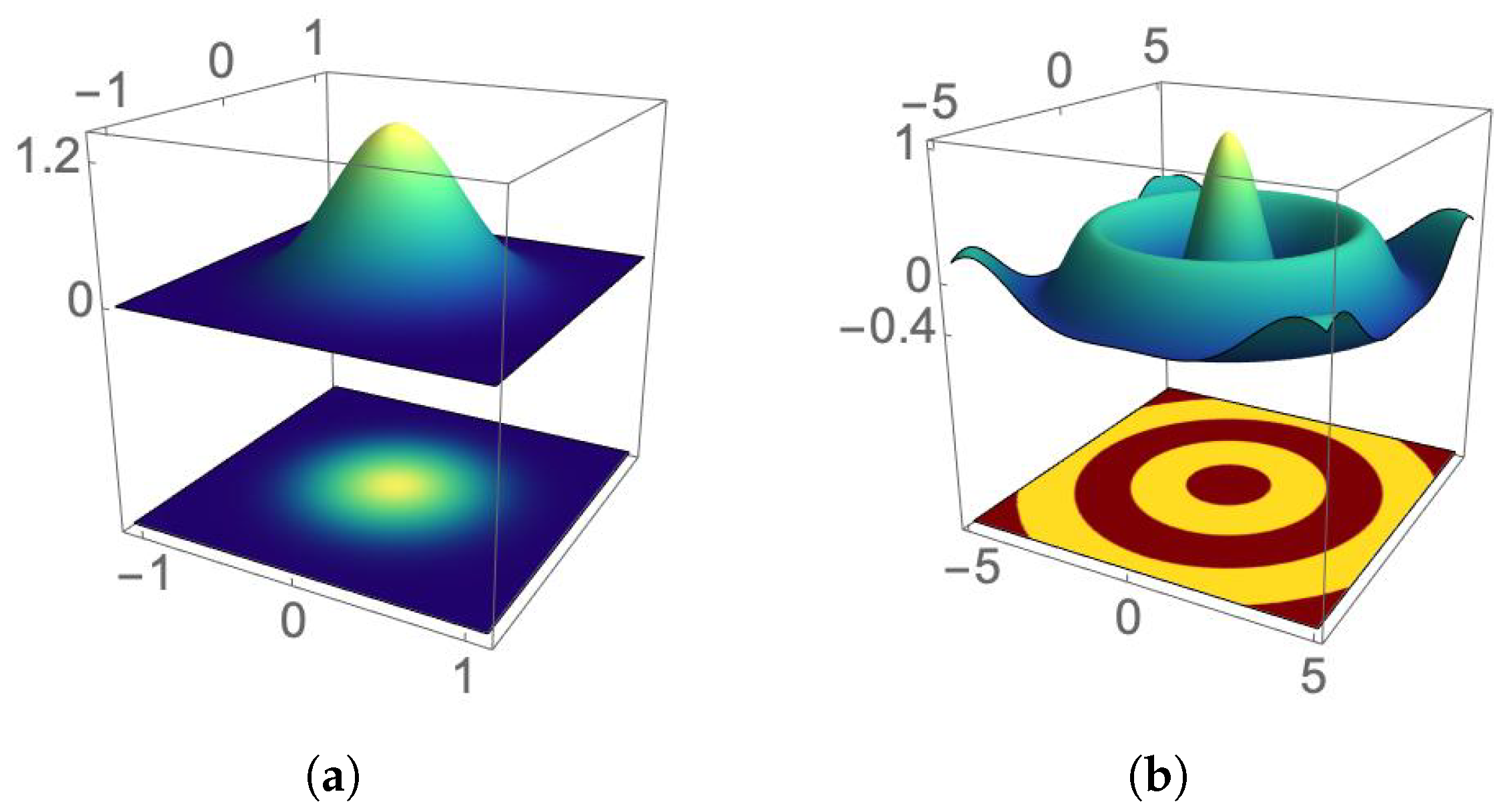
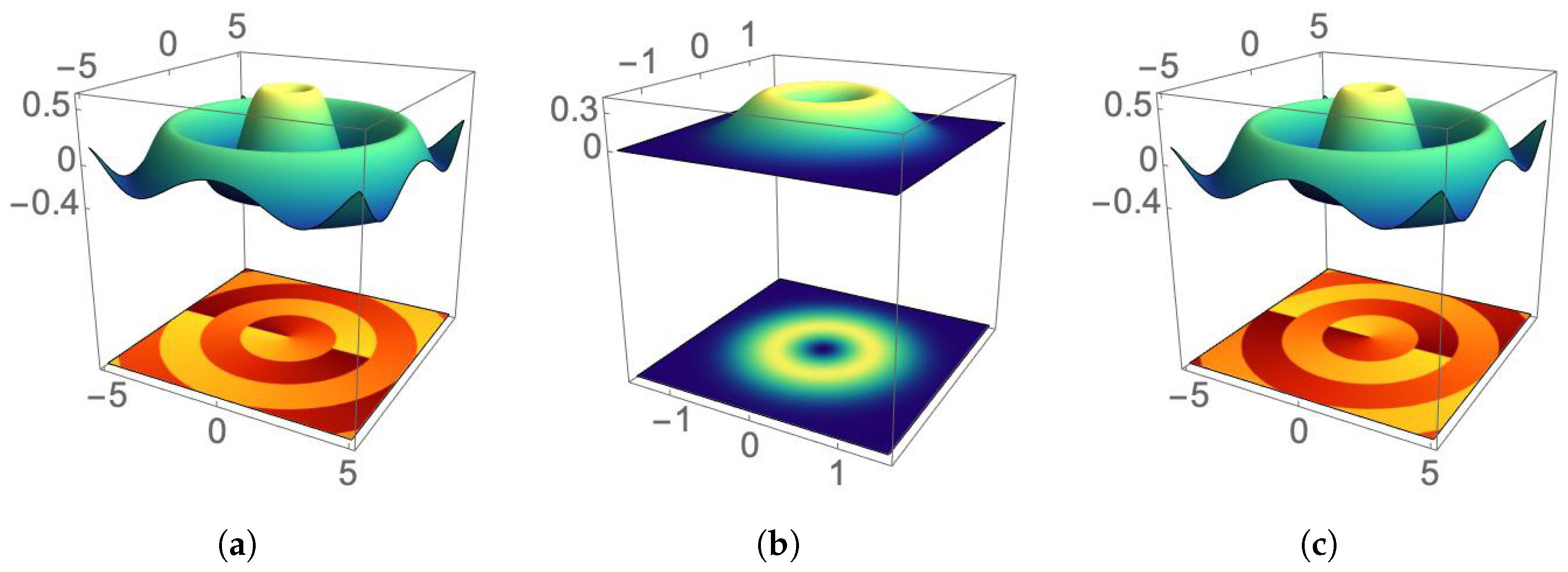
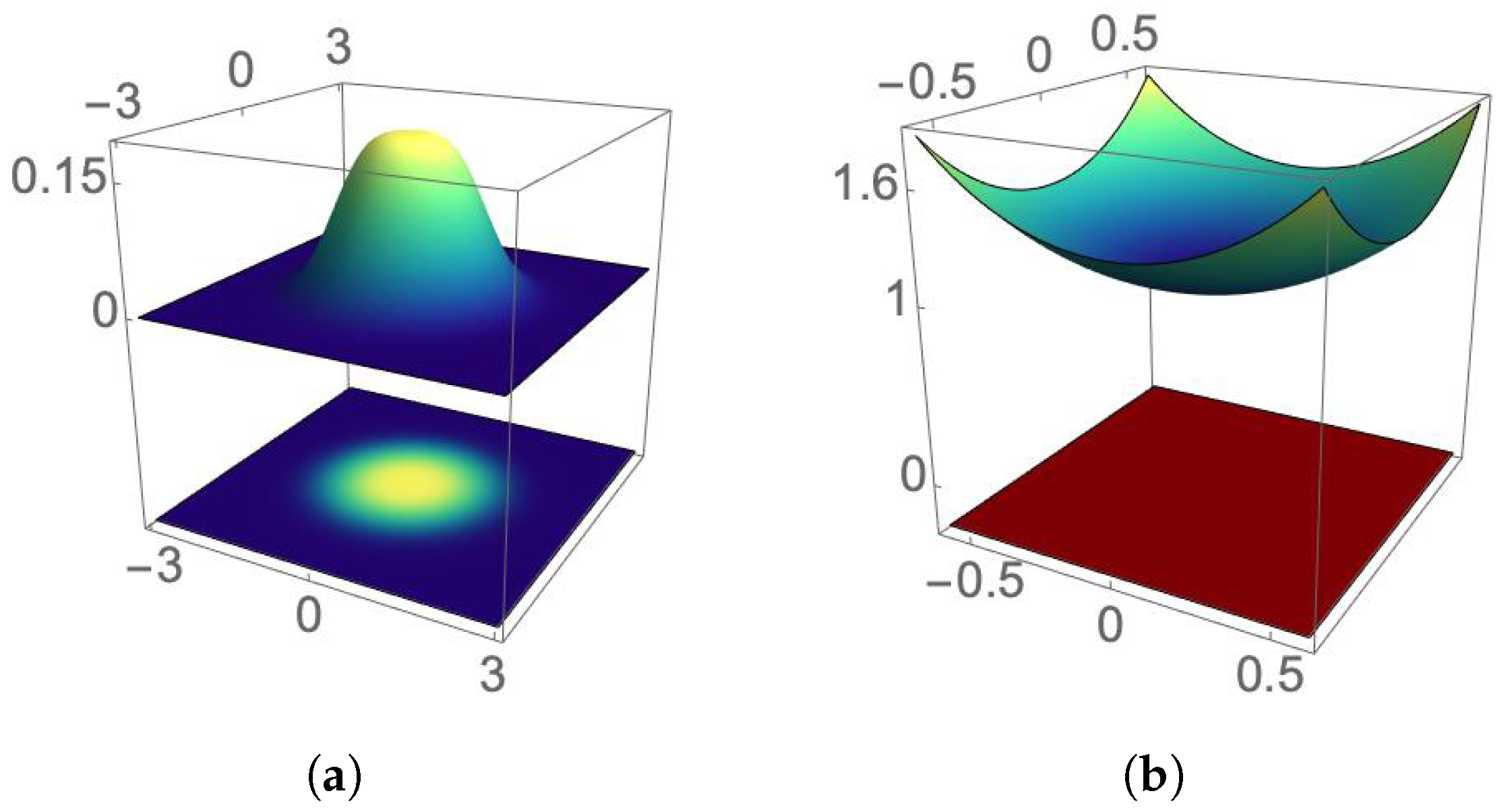
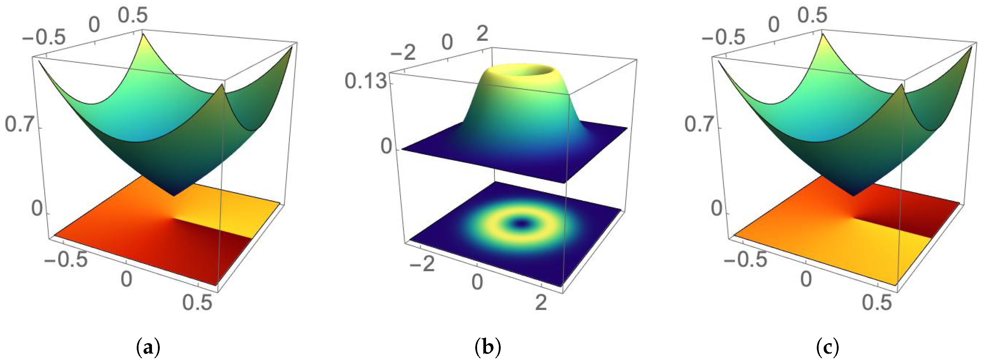
• Maximum spreading of the beam. At the points $z_n=\frac{1}{2}(2n+1)\pi z_R$, with $n\in \mathbb{Z}$, the coherent state $V_{\ell }(\mathit{r},z;\xi )$ changes its profile from the Bessel function of the first kind $J_{|\ell |}$ to the modified Bessel function $I_{|\ell |}$. The latter yields the maximum radial uncertainty of the beam. The intensity distribution is blurred on the transverse plane, and the phase distribution occurs without the radial distribution of the previous cases (the Bessel function $I_{\nu }\left(u\right)$ has no zeros along the real axis of the complex u-plane if $\nu$ is an integer [43]). Figure 8 and Figure 9 show the transverse intensity and phase distribution for $\ell =0$ and $\ell =1$, respectively.

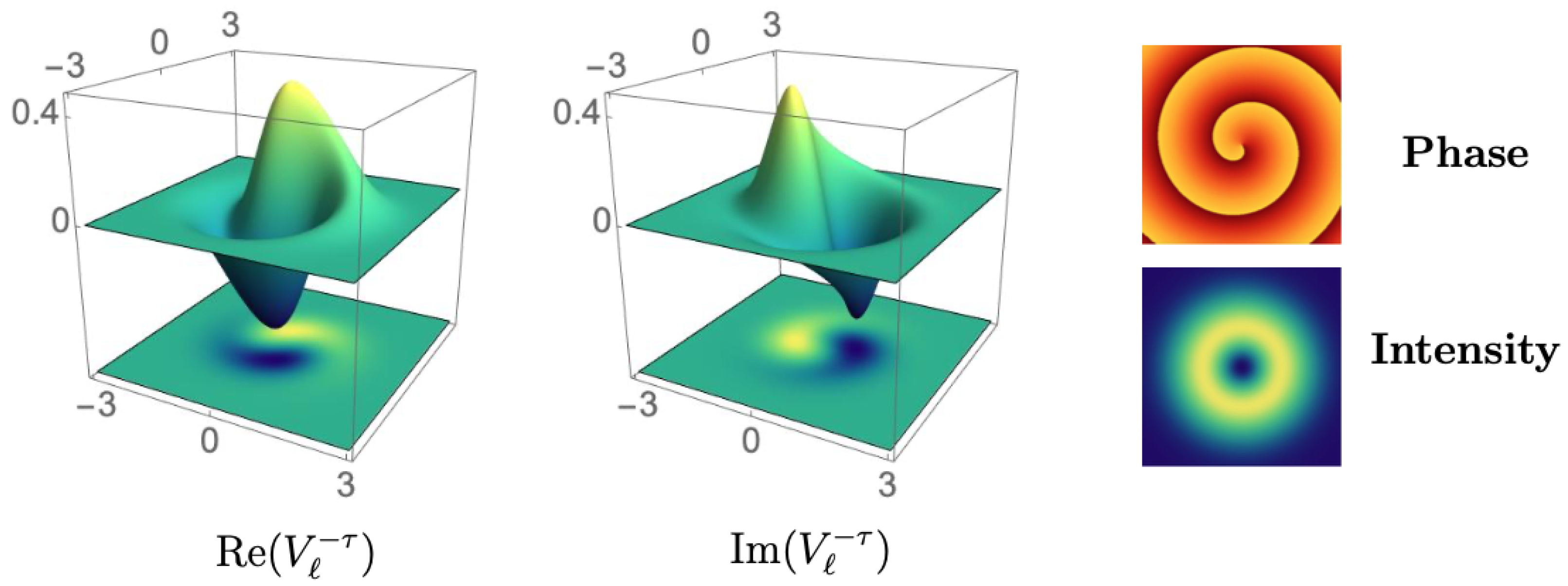
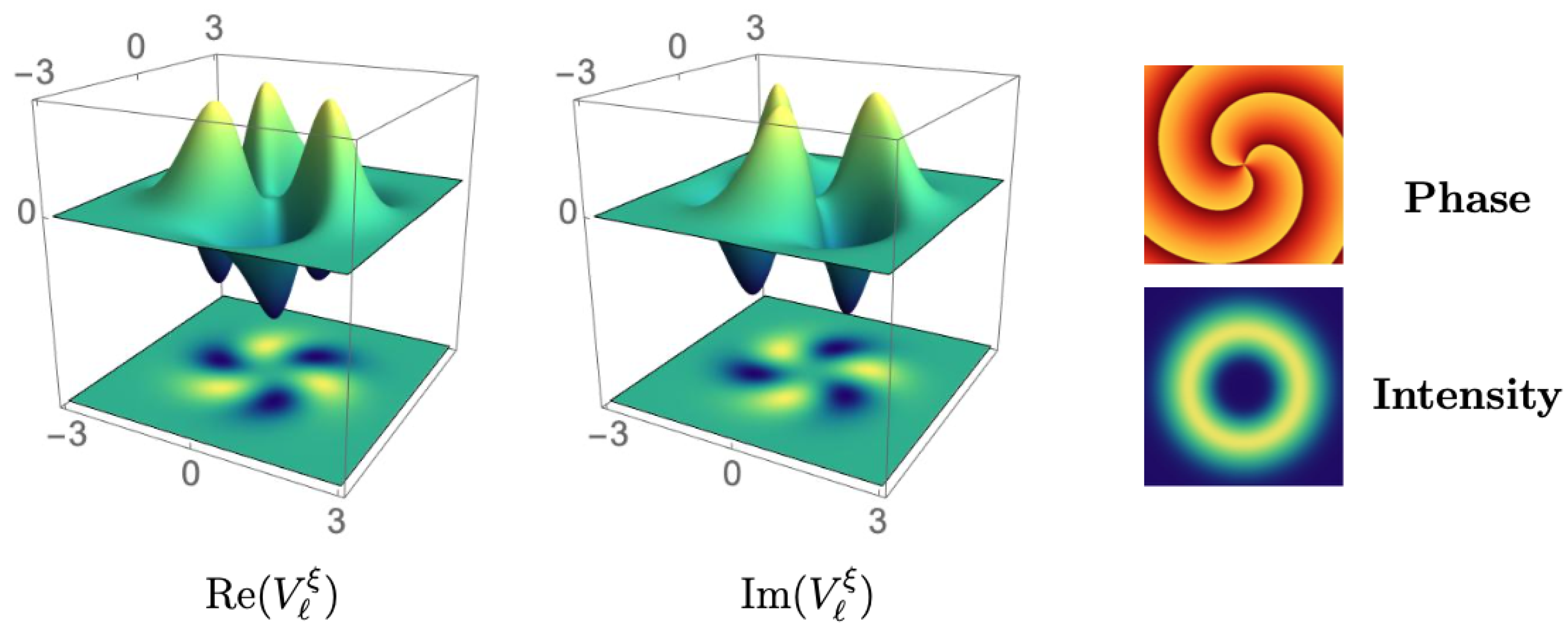
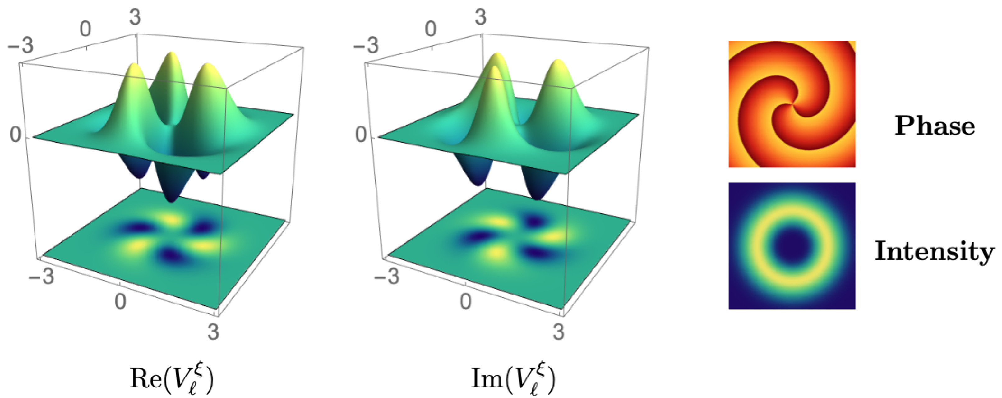
• Vortices. At any other point of the propagation axis, the Bessel function appearing in (10) is complex-valued. Thus, $J_{|\ell |}$ contributes to the global phase of $V_{\ell }(\mathit{r},z;-\tau )$ with a term that depends on $\rho$ in general. As a consequence, the phase distribution of the initial configuration is distorted such that it exhibits vortices. This is illustrated in Figure 10 for $\ell =1$, the real and imaginary parts of $V_1(\mathit{r},z;-\tau )$ change sign in different regions of the transverse plane. The phase distribution is, therefore, characterized by the quotient of such signs.

3.3.2. Behavior for Pure Imaginary Eigenvalues

Making $\xi =-i\tau$ in (8), the modified Bessel function $I_{|\ell |}$ is complex-valued, no matter the value of the propagation variable z. As in the previous case, $I_{|\ell |}$ contributes to the global phase of $V_{\ell }(\mathit{r},z;-i\tau )$ with a term that depends on $\rho$. See Figure 11 and Figure 12.

Figure 11 shows the real and imaginary parts of $V_{\ell }(\mathit{r},z;-i\tau )$ at $z=0$, with $\tau =1/2$. As in the previous case, these functions change signs in different regions of the transverse plane. Please note that the number of local maxima is defined by the value of ℓ; the same holds for the number of local minima (where the functions acquire negative values). The number of vortices in the phase distribution is also determined by ℓ. After the beam propagation, at $z=\frac{\pi }{2}{z}_R$, the distribution of local maxima and minima has changed, as well as the configuration of vortices, see Figure 12.

4. Discussion

We have studied the z-propagation of electromagnetic waves through weakly inhomogeneous media of parabolic refractive index. After imposing the constant beam-width condition, we focused on the electric field of guided Laguerre-Gauss modes propagating along the z-axis with constant width and carrying finite transverse optical power [16]. These exhibit helicity, distinguished by an integer $\ell \ne 0$, which is right-handed if $\ell >0$ and left-handed if $\ell <0$. Modes with no helicity are characterized by $\ell =0$.

The guided Laguerre-Gauss modes (LG modes for short) form an orthonormal basis for the space of solutions $\mathcal{H}$ of the paraxial wave equation and can be grouped according to the helicity parameter ℓ, so they span infinite-dimensional solution subspaces (called hierarchies) ${\mathcal{H}}_{\ell }\subset \mathcal{H}$ such that $\mathcal{H}={⨁}_{\ell }{\mathcal{H}}_{\ell }$.

The most striking feature of this decomposition is that the symmetry underlying the hierarchies ${\mathcal{H}}_{\ell }$ is linked to the simplest noncompact non-Abelian Lie group [60], denoted by $SU(1,1)$. We have shown that the hierarchies ${\mathcal{H}}_{\ell }$ are irreducible representation spaces for the Lie algebra $su(1,1)$, we have also identified the differential form of the generators ${\mathcal{L}}_{\ell }$, ${\mathcal{L}}_{\ell }^{\pm }$.

Surprisingly, the LG modes satisfy the eigenvalue equation of ${\mathcal{L}}_{\ell }$ with the corresponding propagation constants playing the role of eigenvalues. In turn, ${\mathcal{L}}_{\ell }^{\pm }$ are ladder operators that connect a certain LG mode to another with eigenvalues stepped by one unit. These results mean that the Lie algebra $su(1,1)$ determines the way the LG modes propagate along the z-axis.

Following the notion of coherent states introduced by Barut and Girardello [50], in each hierarchy ${\mathcal{H}}_{\ell }$, we have constructed a linear superposition of LG modes that is eigenfunction of ${\mathcal{L}}_{\ell }^{-}$ with complex eigenvalue $\xi =\tau e^{-i\varphi }$. These generalized coherent states are nothing more than guided Bessel–Gauss modes (BG modes) carrying finite transverse optical power that propagate with a well-defined optical angular momentum and self-focus along the z-axis. The phase $\varphi =arg\left(\xi \right)$ characterizes the profile of the mode (either $J_{|\ell |}$ or $I_{|\ell |}$), while the modulus $\tau =\left|\xi \right|$ is responsible for its quality.

We have found that by setting $\tau$ close to zero, the BG modes so constructed are as Gaussian as the limit $\tau \to 0$ allows. With this in mind, to evaluate the quality of a signal that is represented by any of these modes, we have analyzed the transverse-spread ${\sigma }_{\mathit{r}}{\sigma }_{\mathit{p}}$ of measuring the joint variability of the transverse-position $\mathit{r}$ and the transverse-propagation direction $\mathit{p}$. The Robertson inequality [52] produces a result that depends sinusoidally on the propagation variable z and is such that the smaller $\tau$, the shorter the difference ${\sigma }_{\mathit{r}}{\sigma }_{\mathit{p}}{{|}_{max}-{\sigma }_{\mathit{r}}{\sigma }_{\mathit{p}}|}_{min}$. In turn, the Schrödinger inequality [56] removes the dependence on z by providing ${\sigma }_{\mathit{r}}{\sigma }_{\mathit{p}}{|}_{min}$ only.

Using the above results, to determine how close a BG mode is to an ideal Gaussian beam, we have introduced the quantity $M_{\ell }^2\left(\tau \right)=k_0{\sigma }_{\mathit{r}}{\sigma }_{\mathit{p}}{|}_{min}=2\sqrt{{\langle {\mathcal{L}}_{\ell }\rangle }^2-{\tau }^2}\ge 1$, where $\langle {\mathcal{L}}_{\ell }\rangle$ is the expectation value of ${\mathcal{L}}_{\ell }$. It is remarkable that $M_{\ell }^2\left(\tau \right)$ coincides with the notion of the beam propagation factor (also called beam quality factor) ${\mathcal{M}}^2$ [44,45], the most important feature describing the quality of light beams [46,47].

It is necessary to emphasize that both the Robertson and the Schrödinger inequalities are commonly used in quantum mechanics but rarely reported in connection with the beam quality factor ${\mathcal{M}}^2$. Remarkable exceptions are [59], where it is suggested a link between some invariant quantities and generalized uncertainty relations like the Schrödinger one, and [24], where the ${\mathcal{M}}^2$ factor of Hermite-Gauss modes is directly related to the Schrödinger inequality for $\mathit{r}$ and $\mathit{p}$.

Our expression for ${\mathcal{M}}^2$ is in complete agreement with the results reported in, e.g., [32], where generic BG beams are studied. The authors of [32] develop a direct calculation of the second-order moments associated with the intensity distributions at the waist plane and in the far field, denoted ${\sigma }_0$ and ${\sigma }_{\infty }$ respectively, to write ${\mathcal{M}}^2=2\pi {\sigma }_0{\sigma }_{\infty }$. However, using algebraic techniques, without cumbersome calculations involved, with $M_{\ell }^2\left(\tau \right)$ we have introduced a simple and elegant way to evaluate ${\mathcal{M}}^2$ in terms of $\tau$, the modulus of the complex parameter $\xi$ that characterizes the BG modes as generalized coherent states.

Clearly, not only the profile and the way the BG modes propagate along the z-axis but also their quality is determined by the underlying symmetry of the hierarchy ${\mathcal{H}}_{\ell }$. This conclusion would not be clear without transferring notions that are quite natural in quantum mechanics to the field of optics. In particular, the construction of ladder operators for LG modes that have a well-defined optical angular momentum allows the creation of linear superpositions of them, whose coherence properties can be maximized to generate BG modes as generalized coherent states for the Lie algebra $su(1,1)$.

From the experimental point of view, our BG modes may be produced as the result of the interference of a Gaussian beam with itself [61] by means of all the available techniques to generate some other BG beams. These include, for instance, the assemblies of circular slits and focusing lenses [36] and the use of conical lenses (also called axicons) [62].

5. Conclusions

Summarizing some of the most notable coherence properties of the BG modes reported in this work, we have:

∘

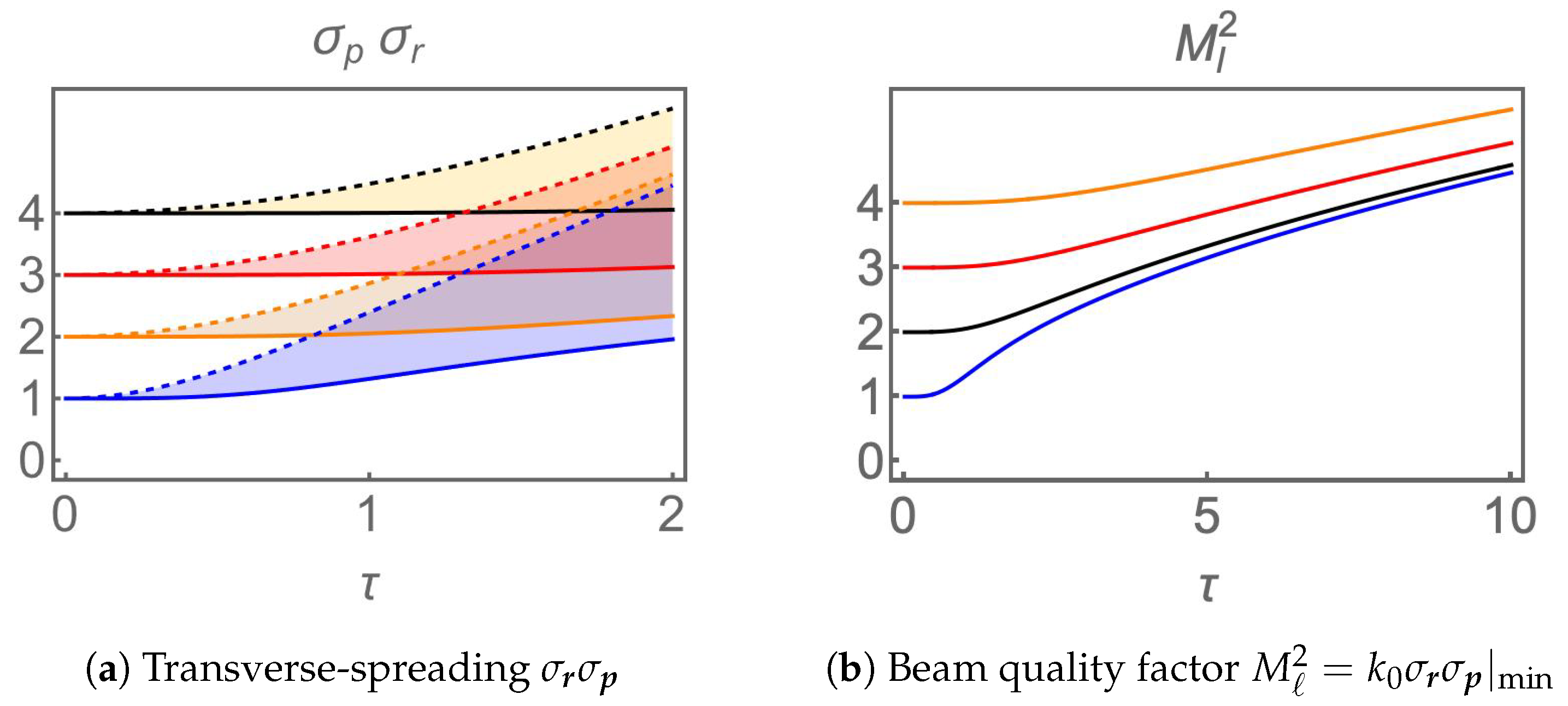
The maximum transverse-spreading of any BG mode is parameterized by $\tau =\left|\xi \right|$. The shorter the value of $\tau$, the better the collimation of the corresponding beam.

∘

The quality of the BG modes is also parameterized by $\tau$: the shorter the value of $\tau$, the closer the BG modes are to the Gaussian profile.

∘

The optical angular momentum $\ell \hslash$ spoils the beam quality: poor beam quality results for large $|\ell |$, no matter how small $\tau$ is.

∘

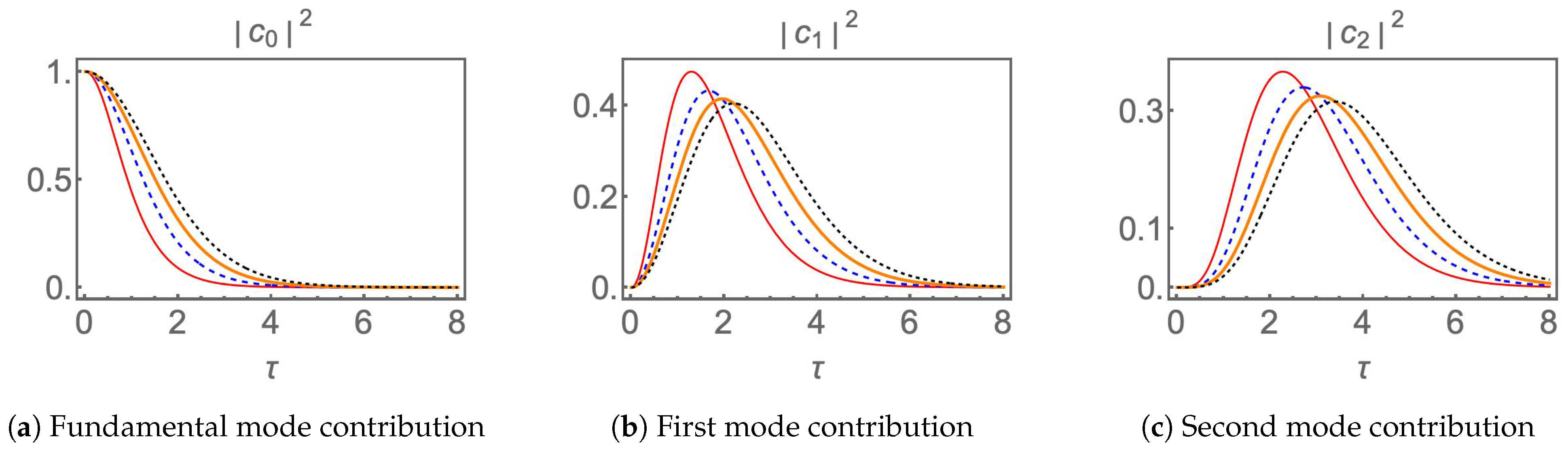
The fundamental LG mode is dominant in any superposition intended to build high-quality BG modes. The contribution of the remaining LG modes can be treated as a disturbance (noise) that deviates the BG mode from the ideal Gaussian profile.

∘

The profile of the BG mode is $I_{|\ell |}$ for $\varphi =arg\left(\xi \right)=0$, and $J_{|\ell |}$ for $\varphi =-\pi$.

∘

No matter the value of $\varphi$, the profile of the BG modes changes periodically from $I_{|\ell |}$ to $J_{|\ell |}$ as the beam propagates along the z-axis.

∘

The transverse-spreading of the BG modes is always finite and changes periodically from its maximum value to its minimum value at very specific points along the propagation axis.

∘

At any other point of the propagation axis, the phase distribution of the BG modes exhibits vortices.

All these properties are the result of constructing the BG modes as generalized coherent states for the Lie algebra $su(1,1)$, in terms of the irreducible representation spanned by LG modes that have a well-defined optical angular momentum.

Like other BG beam models, our generalized coherent states could find applications in optical engineering. For example, to design secure communication protocols [38,39] or improve efficiency in laser writing, such as micro-machining [61,62] and Bragg grating inscription on materials [63]. Higher-order BG beams are also efficient for controlling light filamentation in nonlinear materials [64] and for designing optical tweezers [21]. For applications in the quantum domain, since optical angular momentum can be entangled [20], the BG modes are more suitable for generating and studying entanglement in SPDC processes [65].

It is feasible to use other linear superpositions of LG modes to construct additional coherent states, this time in terms of the Lie group $SU(1,1)$, in the sense proposed by Perelomov [60]. In this case, it is well known that there will be several types of coherent states since $SU(1,1)$ has several series of unitary irreducible representations. The analysis of the coherence properties of the resulting modes can be achieved by following the procedure developed in this article. Work is underway in this direction and will be reported elsewhere.

References

1. Barnett, S.M.; Babiker, M.; Padgett, M.J. Optical orbital angular momentum. Philos. Trans. R. Soc. A 2017, 375, 20150444. [Google Scholar] [CrossRef]
2. Yao, A.M.; Padgett, M.J. Orbital angular momentum: Origins, behavior and applications. Adv. Opt. Photonics 2011, 3, 161–204. [Google Scholar] [CrossRef]
3. Barnett, S.M.; Babiker, M.; Padgett, M.J. (Eds.) Theme Issue “Optical Orbital Angular Momentum”; Royal Society: London, UK, 2017; Volume 375. [Google Scholar]
4. Allen, L.; Beijersbergen, M.W.; Spreeuw, R.J.C.; Woerdman, J.P. Orbital angular momentum of light and the transformation of Laguerre-Gaussian laser modes. Phys. Rev. A 1992, 45, 8185–8189. [Google Scholar] [CrossRef]
5. He, H.; Friese, M.E.J.; Heckenberg, N.R.; Rubinsztein-Dunlop, H. Direct Observation of Transfer of Angular Momentum to Absorptive particles from a Laser Beam with a Phase Singularity. Phys. Rev. Lett. 1995, 75, 826–829. [Google Scholar] [CrossRef] [PubMed]
6. Allen, L.; Padgett, M.J. The Poynting vector in Laguerre-Gaussian beams and the interpretation of their angular momentum density. Opt. Commun. 2000, 184, 67–71. [Google Scholar] [CrossRef]
7. Padgett, M.; Allen, L. Light with a twist in its tail. Contemp. Phys. 2000, 41, 275–285. [Google Scholar] [CrossRef]
8. Barnett, S.M. Optical angular momentum flux. J. Opt. B Quantum Semiclass Opt. 2002, 4, S7–S16. [Google Scholar] [CrossRef]
9. Chaturvedi, A.S.; Mukunda, N. On ‘Orbital’ and ‘Spin’ Angular Momentum of Light in Classical and Quantum Theories—A General Framework. Fortschr. Phys. 2018, 66, 1800040. [Google Scholar]
10. Bazhenov, V.Y.; Soskin, M.S.; Vasnetsov, M.V. Screw dislocations in light wavefronts. J. Mod. Opt. 1992, 39, 985–990. [Google Scholar] [CrossRef]
11. Beijersbergen, M.W.; Allen, L.; van der Veen, H.E.L.; Woerdman, J.P. Astigmatic mode converters of orbital angular momentum. Opt. Commun. 1993, 96, 123–132. [Google Scholar] [CrossRef]
12. Arlt, J.; Dholakia, K.; Allen, L.; Padgett, M.J. The production of multiringed Laguerre-Gaussian modes by computer-generated holograms. J. Mod. Opt. 1997, 45, 1231–1237. [Google Scholar] [CrossRef]
13. Ngcobo, S.; Aït-Ameur, K.; Passilly, N.; Hasnaoui, A.; Forbes, A. Exciting higher-order radial Laguerre-Gaussian modes in a dipole-pumped solid-state laser resonator. Appl. Opt. 2013, 52, 2093–2101. [Google Scholar] [CrossRef] [PubMed]
14. Forbes, A.; Dudley, A.; McLaren, M. Creation and detection of optical modes with spacial light modulators. Adv. Opt. Photonics 2016, 8, 200–227. [Google Scholar] [CrossRef]
15. Cruz y Cruz, S.; Escamilla, N.; Velázquez, V. Generation of Sources of Light with Well Defined Orbital Angular Momentum. J. Phys. Conf. Ser. 2016, 698, 012016. [Google Scholar] [CrossRef]
16. Cruz y Cruz, S.; Gress, Z.; Jiménez-Macías, P.; Rosas-Ortiz, O. Laguerre-Gaussian Wave propagation in Parabolic Media. In Geometric Methods in Physics XXXVIII; Trends in Mathematics Birkhäuser: Cham, Switzerland, 2020; pp. 117–128. [Google Scholar]
17. Gress-Mendoza, Z.; Cruz y Cruz, S.; Velázquez, V. Production and Characterization of Helical Beams by means of Diffraction Gratings. J. Phys. Conf. Ser. 2023, 2448, 012017. [Google Scholar] [CrossRef]
18. Willner, A.E.; Ren, Y.; Xie, G.; Yan, Y.; Li, L.; Zhao, Z.; Wang, J.; Tur, M.; Molisch, A.F.; Ashrafi, S. Recent advances in high-capacity free-space optical and radio-frequency communications using orbital angular momentum multiplexing. Philos. Trans. R. Soc. A 2017, 375, 20150439. [Google Scholar] [CrossRef] [PubMed]
19. Russell, P.S.; Beravat, R.; Wong, G.K.L. Helically twisted photonic crystal fibres. Philos. Trans. R. Soc. A 2017, 375, 20150440. [Google Scholar] [CrossRef]
20. Krenn, M.; Malik, M.; Erhard, M.; Zeilinger, A. Orbital angular momentum of photons and the entanglement of Laguerre-Gaussian modes. Philos. Trans. R. Soc. A 2017, 375, 20150442. [Google Scholar] [CrossRef]
21. Yang, Y.; Ren, Y.-X.; Chen, M.; Arita, Y.; Rosales-Guszmán, C. Optical trapping with structured light: A review. Adv. Photonics 2021, 3, 034001. [Google Scholar] [CrossRef]
22. Kotlyar, V.V.; Kovalev, A.A.; Nalimov, A.G. Propagation of hypergeometric laser beams in a medium with a parabolic refractive index. J. Opt. 2013, 15, 125706. [Google Scholar] [CrossRef]
23. Petrov, N.I. Spin-Dependent Transverse Force on a Vortex Light Beam in an Inhomogeneous Medium. JETP Lett. 2016, 13, 443–448. [Google Scholar] [CrossRef]
24. Cruz y Cruz, S.; Gress, Z. Group approach to the paraxial propagation of Hermite-Gaussian modes in a parabolic medium. Ann. Phys. 2017, 383, 257–277. [Google Scholar] [CrossRef]
25. Wu, Y.; Wu, J.; Lin, Z.; Fu, X.; Qiu, H.; Chen, K.; Deng, D. Propagation properties and radiation forces of the Hermite-Gaussian vortex beam in a medium with a parabolic refractive index. Appl. Opt. 2020, 59, 8342–8348. [Google Scholar] [CrossRef] [PubMed]
26. Puttnam, B.J.; Rademacher, G.; Luís, R.S. Space-division multiplexing for optical fiber communications. Optica 2021, 8, 1186–1203. [Google Scholar] [CrossRef]
27. Siegman, A.E. Lasers; California University Science Books: Melville, NY, USA, 1986. [Google Scholar]
28. Durnin, J. Exact solutions for nondiffracting beams I The scalar theory. J. Opt. Soc. Am. A 1987, 4, 651. [Google Scholar] [CrossRef]
29. Durnin, J.; Miceli, J.; Eberly, J. Diffraction-free beams. Phys. Rev. Lett. 1987, 58, 1499. [Google Scholar] [CrossRef] [PubMed]
30. Gori, F.; Guattari, G.; Padovani, C. Bessel-Gauss beams. Opt. Commun. 1987, 64, 491. [Google Scholar] [CrossRef]
31. Bagini, V.; Frezza, F.; Santarsiero, M.; Schettini, G.; Schirripa Spagnolo, G. Generalized Bessel-Gauss beams. J. Mod. Opt. 1996, 43, 1155–1166. [Google Scholar]
32. Borghi, R.; Santarsiero, M. M2 factor of Bessel-Gauss beams. Opt. Lett. 1997, 22, 262–264. [Google Scholar] [CrossRef]
33. Li, Y.; Lee, H.; Wolf, E. New generalized Bessel-Gaussian beams. J. Opt. Soc. Am. A 2004, 21, 640–646. [Google Scholar] [CrossRef]
34. Stoyanov, L.; Stefanov, A.; Dreischuh, A.; Paulus, G.G. Gouy phase of Bessel-Gaussian beams: Theory vs. experiment. Opt. Express 2023, 31, 13683–13699. [Google Scholar] [CrossRef]
35. Wolf, K.B. Diffraction-Free Beams Remain Diffraction Free under All Paraxial Optical Transformations. Phys. Rev. Lett. 1988, 60, 757–759. [Google Scholar] [CrossRef] [PubMed]
36. Uehara, K.; Kikuchi, H. Generation of Nearly Diffraction-Free Laser Beams. Appl. Phys. B 1989, 48, 125–129. [Google Scholar] [CrossRef]
37. Overfelt, P.L. Bessel-Gauss pulses. Phys. Rev. A 1991, 44, 3941–3947. [Google Scholar] [CrossRef] [PubMed]
38. Wang, T.-L.; Gariano, J.A.; Djordjevic, I.B. Employing Bessel-Gaussian Beams to Improve Physical-Layer Security in Free-Space Optical Communications. IEEE Photonics J. 2018, 10, 7907113. [Google Scholar] [CrossRef]
39. Wang, W.; Zhang, G.; Ye, T.; Wu, Z.; Bai, L. Scintillation of the orbital angular momentum of a Bessel-Gaussian beam and its application on multi-parameter multiplexing. Opt. Express 2023, 31, 4507–4520. [Google Scholar] [CrossRef]
40. Doster, T.; Watnik, A.T. Laguerre-Gauss and Bessel-Gauss beams propagation through turbulence: Analysis of channel efficiency. Appl. Opt. 2016, 55, 10239–10246. [Google Scholar] [CrossRef]
41. Gress, Z.; Cruz y Cruz, S. A Note on the Off-Axis Gaussian Beams Propagation in Parabolic Media. J. Phys. Conf. Ser. 2017, 839, 012024. [Google Scholar] [CrossRef]
42. Gress, Z.; Cruz y Cruz, S. Hermite Coherent States for Quadratic Refractive Index Optical Media, In Integrability, Supersymmetry and Coherent States; Kuru, S., Negro, J., Nieto, L.M., Eds.; CRM Series in Mathematical Physics; Springer: Berlin/Heidelberg, Germany, 2019; pp. 323–339. [Google Scholar]
43. Olver, F.W.J.; Lozier, D.W.; Boisvert, R.F.; Clark, C.W. (Eds.) NIST Handbook of Mathematical Functions; Cambridge University Press: Cambridge, UK, 2010. [Google Scholar]
44. Siegman, A.E. New developments in laser resonators. SPIE 1990, 1224, 1. [Google Scholar]
45. Siegman, A.E. Defining, measuring, and optimizing laser beam quality. SPIE 1993, 1868, 1. [Google Scholar]
46. Bélanger, P.-A.; Champagne, Y.; Paré, C. Beam propagation factor of diffracted laser beams. Pot. Commun. 1994, 105, 233. [Google Scholar] [CrossRef]
47. Saleh, B.E.A.; Teich, M.C. Fundamentals of Photonics, 2nd ed.; John Wiley: Hoboken, NJ, USA, 2007. [Google Scholar]
48. Glauber, R.J. Quantum Theory of Optical Coherence; Selected Papers and Lectures; Wiley-VCH: Weinheim, Germany, 2007. [Google Scholar]
49. Rosas-Ortiz, O. Coherent and Squeezed States: Introductory Review of Basic Notions, Properties, and Generalizations. In Integrability, Supersymmetry and Coherent States; Kuru, S., Negro, J., Nieto, L.M., Eds.; CRM Series in Mathematical Physics; Springer: Berlin/Heidelberg, Germany, 2019; pp. 187–230. [Google Scholar]
50. Barut, A.O.; Girardello, L. New “coherent” states associated with non-compact groups. Commun. Math. Phys. 1971, 21, 41. [Google Scholar] [CrossRef]
51. Gradshteyn, I.S.; Ryzhik, I.M. Table of Integrals, Series, and Products, 7th ed.; Academic Press: Burlington, MA, USA, 2007. [Google Scholar]
52. Robertson, H.P. The Uncertainty Principle. Phys. Rev. 1929, 34, 163. [Google Scholar] [CrossRef]
53. Kennard, E.H. Zur quanten mechanik einfacher bewegungstypen. Z. Phys. 1929, 44, 326. [Google Scholar] [CrossRef]
54. Gloge, D.; Marcuse, D. Formal Quantum Theory of Light Rays. J. Opt. Soc. Am. 1969, 59, 1629. [Google Scholar] [CrossRef]
55. Stoler, D. Operator methods in physical optics. J. Opt. Soc. Am. A 1981, 71, 334. [Google Scholar] [CrossRef]
56. Schrödinger, E. E Zum Heisenberschen Unsch"afprinzip. Ber. Kgl. Akad. Wiss. Berlin 1930, 24, 296. [Google Scholar]
57. Bandres, M.A.; López-Mago, D.; Gutérrez-Vega, J.C. Higher order moments and overlaps of rotationally symmetric beams. J. Opt. 2010, 12, 015706. [Google Scholar] [CrossRef]
58. Martínez-Herrero, R.; Manjavacas, A. Overall second-order parametric characterization of light beams propagating through spiral phase elements. Opt. Commun. 2009, 282, 473. [Google Scholar] [CrossRef]
59. Dodonov, V.V.; Man’ko, O.V. Universal invariants of quantum-mechanical and optical systems. J. Opt. Soc. Am. A 2000, 17, 2403. [Google Scholar] [CrossRef] [PubMed]
60. Perelomov, A. Generalized Coherent States and Their Applications; Springer: Berlin, Germany, 1986. [Google Scholar]
61. Beuton, R.; Chimier, B.; Quinoman, P.; González Alaiza de Martínez, P.; Nuter, R.; Duchateau, G. Numerical studies of dielectric material modifications by a femtosecond Bessel-Gauss laser beam. Appl. Phys. A 2021, 127, 334. [Google Scholar] [CrossRef]
62. Baltrukonis, J.; Ulčinas, O.; Orlov, S.; Jukna, V. High-Order Vector Bessel-Gauss Beams for Laser Micromachining of Transparent Materials. Phys. Rev. Appl. 2021, 16, 034001. [Google Scholar] [CrossRef]
63. Harb, J.; Talbot, L.; Petit, Y.; Bernier, M.; Canioni, L. Demonstration of Type A volume Bragg gratings inscribed with a femtosecond Gaussian-Bessel laser beam. Opt. Express 2023, 31, 15736–15746. [Google Scholar] [CrossRef] [PubMed]
64. Miller, J.K.; Tsvetkov, D.; Terekhov, P.; Litchinitser, N.M.; Dai, K.; Free, J.; Johnson, E.G. Spatio-temporal controlled filamentation using higher order Bessel-Gaussian beams integrated in time. Opt. Express 2021, 29, 19362–19372. [Google Scholar] [CrossRef]
65. McLaren, M.; Agnew, M.; Leach, J.; Roux, F.S.; Padgett, M.J.; Boyd, R.W.; Forbes, A. Entangled Bessel-Gaussian Beams. Opt. Express 2012, 20, 23589–23597. [Google Scholar] [CrossRef]
66. Finney, R.L.; Ostberg, D.R. Elementary Differential Equations with Linear Algebra; Addison-Wesley: Boston, MA, USA, 1976. [Google Scholar]
67. Negro, J.; Nieto, L.M.; Rosas-Ortiz, O. Confluent hypergeometric equations and related solvable potentials in Quantum Mechanics. J. Math. Phys. 2000, 41, 7964. [Google Scholar] [CrossRef]
68. Negro, J.; Nieto, L.M.; Rosas-Ortiz, O. Refined Factorizations of Solvable Potentials. J. Phys. A Math. Gen. 2000, 33, 7207. [Google Scholar] [CrossRef]
69. deLange, O.L.; Raab, R.E. Operator Methods in Quantum Mechanics; Clarendon Press: Oxford, UK, 1992. [Google Scholar]
70. Miller, W. Lie Theory and Special Functions; Academic Press: New York, NY, USA, 1968. [Google Scholar]
71. Gilmore, R. Lie Groups, Lie Algebras and Some of Their Applications; Kriege: Malabar, FL, USA, 1994. [Google Scholar]
72. Infeld, L.; Hull, T.E. The Factorization Method. Rev. Mod. Phys. 1951, 23, 21. [Google Scholar] [CrossRef]
73. Mielnik, B.; Rosas-Ortiz, O. Factorization: Little or great algorithm? J. Phys. A Math. Gen. 2004, 37, 10007. [Google Scholar] [CrossRef]
Figure 1. The propagation constant (3) is ( n + 1 )-fold degenerate for n = | | + 2 p = fixed . In such a case we write β | | p β ( n ) = n + 1 (horizontal arrays). For = fixed , the admissible values of β | | p are equidistant, with steps of two units (vertical arrays). In general, the entire set { β | | p } may be counted by a one-to-one correspondence with the energy spectrum of a two-dimensional harmonic oscillator in the quantum domain.
Photonics 10 01162 g001
Figure 3. The harmonics labeled with small p contribute more significantly to increasing the quality of the BG mode. By setting τ close to zero, the main contribution is provided by the fundamental mode (a). The remaining harmonics (figures (b,c) show p = 1 and p = 2 ) contribute by perturbing the fundamental harmonic in such a way that the BG mode deviates from the ideal Gaussian profile. The color-code is the same as in Figure 2.
Photonics 10 01162 g003
Figure 4. The transverse-spreading σ r σ p introduced in (14) for the Bessel–Gauss coherent states V ( r , z ; ξ ) oscillates between the extreme values σ r σ p | max and σ r σ p | min , dashed and continuous curves, respectively. The areas between these values are shadowed to facilitate the comparison of results (a). The function σ r σ p | max also refers to the mean energy and the quadrature deviations, compare (a) with Figure 2. The minimal value σ r σ p | min is directly proportional to the M 2 factor (18), plotted in (b). In all cases, the curves correspond to = 3 , 2 , 1 , 0 (from top to bottom). The horizontal and vertical axis are in units of τ and k 0 1 , respectively. The lowest bound defined by both the Robertson and the Schrödinger inequalities, is attained at τ = 0 for = 0 , written σ r σ p | Gauss = k 0 1 .
Photonics 10 01162 g004
Figure 5. Intensity of the BG coherent states V ( r , z ; ξ ) introduced in (8), from the longitudinal perspective, for ξ = τ and the indicated values of τ . The function V ( r , z ; ξ ) is periodic with period 2 π z R . Collimation: The beam is better collimated for small values of τ . Self-focusing: The configuration at z = 0 , where the radial uncertainty σ r is minimum and the value of σ p as well as intensity are maxima, is recovered at z q = q π z R . In turn, the maximum value of σ r (minimum value of σ p ) and minimum intensity are attained at z n = ( n + 1 2 ) π z R . In both cases, the transverse-spreading σ r σ p reaches its minimum value. Transverse profile: For = 0 the intensity is different from zero at ρ = 0 (upper row), but it cancels at ρ = 0 for | | = 1 (lower row). The behavior for | | 2 is qualitatively equivalent to the case | | = 1 .
Photonics 10 01162 g005
Figure 6. Intensity (a) and phase distribution (b) of the BG coherent state V ( r , z ; ξ ) for = 0 and ξ = 1 / 2 . These configurations occur in the transverse planes defined by the points z 2 q = 2 q π z R . The related profile is characterized by the Bessel function of the first kind J 0 depicted at the right, so the phase distribution is radial, with discontinuities located at the zeros of J 0 that represent a phase shift ± π . The brown zones correspond to positive values of J 0 and identify the phase e 0 = 1 . In turn, the yellow zones represent negative values of J 0 , with phase e i π = 1 .
Photonics 10 01162 g006
Figure 7. Intensity (b) and phase distribution of the coherent state V ( r , z ; ξ ) for ξ = 1 / 2 , with = 1 (a) and = 1 (c). These configurations occur in the transverse planes defined by the points z 2 q = 2 q π z R . The polar phase θ sweeps [ π , π ) once in each of the radial zones defined by the sign of the Bessel function J 1 . Brown and yellow color-codes identify the phases π and π , respectively. The helicity of mode = 1 is clockwise while = 1 is counterclockwise.
Photonics 10 01162 g007
Figure 8. Intensity (a) and phase distribution (b) of the coherent state V ( r , z ; ξ ) for = 0 and ξ = 1 / 2 . These configurations occur in the transverse planes defined by the points z 2 n = 1 2 ( 4 n + 1 ) π z R . The related profile is characterized by the modified Bessel function I 0 , which is positive (this function is depicted at the right). The latter means that in contrast with J 0 , the function I 0 provides no phase shifts to a coherent state (compare with Figure 6). Thus, the brown color-code refers to a phase e 0 = 1 .
Photonics 10 01162 g008
Figure 9. Intensity (b) and phase distribution of the coherent state V ( r , z ; ξ ) for ξ = 1 / 2 , with = 1 (a) and = 1 (c). These configurations occur in the transverse planes defined by the points z 2 n = 1 2 ( 4 n + 1 ) π z R . The polar phase θ sweeps [ π , π ) once in the transverse plane. Brown and yellow color-codes identify the phases π and π , respectively. The helicity of mode = 1 is clockwise while = 1 is counterclockwise.
Photonics 10 01162 g009
Figure 10. Real and imaginary parts of the coherent state V ( r , z ; ξ ) for = 1 , ξ = 1 / 2 and z = π 4 z R . Their contributions to the polar phase produce the vortex shown in the figure at the right, which also shows the field intensity.
Photonics 10 01162 g010
Figure 11. Real and imaginary parts of the BG coherent state V ( r , z ; ξ ) for = 3 , ξ = i / 2 and z = 0 . Their contributions to the polar phase produce the vortex shown in the figure at the right, which also shows the field intensity.
Photonics 10 01162 g011
Figure 12. Real and imaginary parts of the BG coherent state V ( r , z ; ξ ) for = 3 , ξ = i / 2 and z = π 2 z R . Their contributions to the polar phase produce the vortex shown in the figure at the right, which also shows the field intensity.
Photonics 10 01162 g012