Abstract
Optical coherence tomography (OCT) represents a non-invasive, high-resolution cross-sectional imaging modality. Macular edema is the swelling of the macular region. Segmentation of fluid or cyst regions in OCT images is essential, to provide useful information for clinicians and prevent visual impairment. However, manual segmentation of fluid regions is a time-consuming and subjective procedure. Traditional and off-the-shelf deep learning methods fail to extract the exact location of the boundaries under complicated conditions, such as with high noise levels and blurred edges. Therefore, developing a tailored automatic image segmentation method that exhibits good numerical and visual performance is essential for clinical application. The dual-tree complex wavelet transform (DTCWT) can extract rich information from different orientations of image boundaries and extract details that improve OCT fluid semantic segmentation results in difficult conditions. This paper presents a comparative study of using DTCWT subbands in the segmentation of fluids. To the best of our knowledge, no previous studies have focused on the various combinations of wavelet transforms and the role of each subband in OCT cyst segmentation. In this paper, we propose a semantic segmentation composite architecture based on a novel U-net and information from DTCWT subbands. We compare different combination schemes, to take advantage of hidden information in the subbands, and demonstrate the performance of the methods under original and noise-added conditions. Dice score, Jaccard index, and qualitative results are used to assess the performance of the subbands. The combination of subbands yielded high Dice and Jaccard values, outperforming the other methods, especially in the presence of a high level of noise.
1. Introduction
Diabetes is one of the fastest-growing chronic diseases, affecting more than 422 million people, especially in low- and middle-income countries [1]. Diabetic macular edema (DME) is the leading cause of blindness in the middle-aged population [2], and age-related macular degeneration (AMD), which mainly affects the elderly [3] and is an untreatable progressive condition, yields fluid leakage [4], macular cysts [5], and swelling in the central part of the retina. Optical coherence tomography (OCT) is well known in the diagnosis of DME and AMD [4,6].
OCT is a non-invasive imaging modality that extracts high-resolution cross-sectional and volumetric images from biological tissue. This modality has been widely utilized in diagnosing different retinal pathologies [7,8].
A macular cyst (fluid) refers to a sac-like pocket of membranous tissue [9] (Figure 1) and is one of the leading causes of blindness in developed countries [10]. Depending on the location of the cyst, three sub-categories are introduced: intra-retinal fluid (IRF), sub-retinal fluid (SRF), and pigment epithelial detachment (PED) [10]. Determining each sub-class is crucial and discussed clinically [9,10]. Due to the complex structure of the fluid, medical professionals sometimes are unable to accurately locate the site of lesions. Therefore, this leads to missed diagnoses and misdiagnoses and can lead to blindness [11].
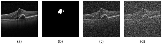
Figure 1.
(a) Original Image; (b) True Mask; (c) Noisy (σ = 80); (d) Noisy (σ = 160). Sample retinal OCT image, mask, and noise-added images with standard deviations of 80 and 160.
Semantic segmentation is a classical method for partitioning an image into regions and assigning a class label to each pixel. Manual OCT image segmentation is often time-consuming and depends on level of expertise [12]. However, automated fluid segmentation from OCT images is a challenging task, due to the particular characteristics of the OCT image and the diverse shapes and locations of the fluids [13,14]. Different approaches have been suggested to tackle this problem. Traditional machine learning methods such as support vector machine (SVM), decision tree [15], and deep learning [13,16] methods have been explored. Deep learning approaches were recently discussed, focusing on input characteristics and using time and frequency transformation [17,18].
Traditional techniques, however, need specific parameters to be defined and manual feature extraction based on expertise. Consequently, the outcomes of these techniques are unsatisfactory. Additionally, there are two distinct areas where deep learning techniques might be enhanced, by including either a new architecture with results close to each other or better network inputs. In addition, the fluid size is often too small in comparison to the background, due to the high noise and artifacts in OCT images; the background region is complex; and the fluid size is too small relative to the background region [19]. We need a robust method that works perfectly for OCT image segmentation. Therefore, we present dual-tree complex wavelet input transform for cyst segmentation in OCT mages, based on a deep learning framework to resolve these problems and improve results [11,20].
1.1. Network Architecture Overview
In recent years, deep learning-based approaches, especially convolutional neural networks (CNN) [21,22], have become dominant and achieved outstanding results in different machine vision tasks, such as segmentation, object detection, and classification [23].
One of the first deep learning methods for semantic segmentation based on CNN was fully convolutional networks (FCNs) [24]. Unet [24], Attention Unet [25], and Deeplabv3+ [26] are some examples of cutting-edge deep learning architectures for image segmentation. FCN with a U-shaped model structure has become the gold standard in medical image segmentation. The U-net architecture uses symmetric encoder and decoder paths with skip connections to capture the context in the image and to enable precise localization using transposed convolutions [24].
In recent years, many deep learning techniques have been used to segment retinal layers and lesions. The OPTIMA dataset [27] was utilized in several scenarios to generalize the model, by retraining it. Furthermore, the RETOUCH challenge dataset has been used in a variety of settings. Liu, D. et al. [28] used a fully convolutional network for OCT semantic segmentation on the OPTIMA dataset. As a result, as proven by ReLayNet [29], excellent segmentation of retinal layers improved the precision of segmentation of the OCT fluid. The UCF group [30] suggested a deep CNN ResNet-based pixel categorization architecture. The RMIT group [31] employed a modified U-net model, in conjunction with an adversarial network. Similarly, Lee et al. [32] used the U-net model on a large dataset and obtained excellent results in OCT image segmentation.
Gopinath et al. [33] applied a CNN-based architecture to segment cystoid macular edemas, which included a post-processing phase that used clustering to refine previously detected cystoid areas. Xiaoming Liu et al. [34] presented a novel loss function and attention U-net for tiny cysts.
However, the deep learning-based solutions described above have certain drawbacks. Some of them have to train several networks to identify and segment fluids, which increases the training complexity. Furthermore, most approaches do not take into account the independent and tiny fluid area in macular edema imaging, and the edges are not extracted correctly in the results. Weak robustness to noise is another problem of these methods.
Certain approaches are applied in this paper that have not previously been evaluated in OCT fluid segmentation. Moreover, in this paper, state-of-the-art architectures are compared to each other. Although CNN-based methods have some drawbacks, including the intrinsic locality of convolution operation, these approaches have excellent representation ability. We applied different and other gold-standard study methods to select the best model, as a base for testing different subbands. The variants of U-net [24], such as Attention Unet [25], Unet+++ [35], R2 Unet [36], Trans-Unet [37], Swin Unet [38], and [28,32,34] were implemented to obtain the best performance for analyzing the effect of different input transform combinations. To address these issues, we used DTCWT’s various subband combinations.
1.2. Input Image Transformations Overview
For better use of image features, we applied the selected model in the transform domain and proposed using different DTCWT combinations to improve the performance of the semantic segmentation method for clean and noisy OCT images.
This study focused on the various combinations of DTCWT and the roles of each subband’s combination in OCT cyst semantic segmentation. In this article, for different types of input subband model (i.e., concatenation, undecimation, separation, etc.), the effects of different inputs were examined in terms of multiple performance metrics, such as the Jaccard index and Dice scores. As far as we know, to date, no study has compared these different transformation inputs in OCT images. Thus, we present a comprehensive comparison study on applying different DTCWT subbands, to find the best input model in cyst segmentation for noisy and regular conditions.
In recent decades, the wavelet transform has become an effective time-frequency analysis tool that decomposes a signal at different timescales using a family of basic functions [39]. DTCWT subbands better preserve edges in the image, while having a low computational complexity compared with other X-lets, and have been utilized in several promising applications [40]. Generally, wavelet transforms allow an improved time-frequency analysis of data and have been successfully applied to deep learning segmentation tasks [39]. X-lets are implemented in two techniques in the deep learning framework: (1) First, they are used in the network architecture; for example, wavelet layers were applied instead of the pooling layer. (2) Sparse wavelet representations of the image are directly used as the input of the network.
Changing the network structure with the wavelet transform has been used to try to remedy pooling problems. Conventional downsampling methods such as max-pooling and average pooling usually ignore the classic Nyquist sampling theorem [41]. Anti-aliased CNNs [42] integrate the wavelet transform with the deep networks, increasing the segmentation accuracy. Hongya Lu et al. used DTCWT-based CNN to segment human thyroid applications. They tried to apply DTCWT in CNN layers, instead of the max-pooling layer [40]. Similarly, Qiufu Li et al. proposed a modified U-net model accompanied by a wavelet layer named Wavenet [41]. Andréde Souza Brito et al. combined max-pooling and wavelet pooling for better performance results [43]. This team suggested a new multi-pooling strategy mixing wavelet and traditional pooling. Alijamaat et al. tried to fuse wavelet pooling and Unet to obtain a better performance in semantic segmentation to extract different directions in brain MRI images [44,45]. Guiyi Yang et al. applied wavelet transform in the Attention Unet for concrete crack segmentation [46].
In most of these studies, subbands were implemented in the network structure. However, some works tried to apply subbands as the input image. Yi Zhang et al. utilized a marine raft segmentation network based on Attention U-net [47]. This team tried to use contourlet subbands as the input. Haixia B utilized 3D discrete wavelet transform as the input image for polarimetric SAR images [48].
Regarding the importance of the automated OCT fluid segmentation in previous works, utilizing subband combinations as input to improve the performance of deep learning methods in normal and noisy conditions can be very useful. In addition, analyzing various subband combinations types in a deep learning framework is very beneficial. Accordingly, this paper presents a DTCWT subband combination based on a deep learning framework, to perform OCT fluid segmentation and improve accuracy.
In this article, we try to go beyond the state-of-the-art in various ways:
- To determine the best semantic segmentation structure for fluid regions and fluid segmentation, we implemented different U-net architectures and other state-of-the-art architectures, to find the best structure to utilize semantic segmentation in OCT images.
- DTCWT subbands were used to extract some critical features in the image. In this way, various subbands and different subband features could be merged to achieve a more accurate segmentation performance in regular and noisy cases. The classical subbands with different layers as input images were also described and tested as input images.
2. Materials and Method
Different mixtures of DTCWT subbands were utilized to analyze each combination’s effect and improve the performance in the deep learning framework, with the best input image combination selection for fluid segmentation.
Various deep learning architectures with different subband inputs and conditions were evaluated in this research. These architectures were coded in the Python programming language, and the deep learning models were trained and tested on a machine with 64 GB of RAM, two parallel GEFORCE GTX 1080 Ti GPUs, and an i7 core 7th generation CPU. Cuda version 10 and cuDNN version 7.5 were utilized on PCs. In this section, we first introduce the dataset. We present the different input image combinations, and in the last section, the theoretical basics of the proposed deep neural network method are discussed.
2.1. Dataset
Two disparate datasets were applied to analyze the effect of different DTCWT subband combinations. The first dataset contained 194 B-scans (fluid and normal) from the cirrus or Heidelberg OCT device. This dataset had previously been collected by our team [49]. To improve our performance, we needed to expand our dataset. The Retinal OCT Fluid Challenge (OPTIMA) [27] was combined with our dataset. This dataset contains 356 Cirrus OCT B-cans images with different resolutions, including both normal and fluid images. We resized all images and ground truth masks from the different datasets to 512 × 51 resolutions. Data are available using this link https://github.com/rezadarooei/OCT_fluid_dataset (accessed on 1 December 2022).
Data augmentation techniques such as rotation, shift, and crop were used to enrich our dataset and assess the agreement and repeatability of the proposed method network. The datasets were randomly divided into training and test sets.
The robustness to noise is an essential factor for the evaluation of each method. We incorporated multiple degrees of noise, since Heidelberg images have a low noise power. Different levels of white noise were added to the database images, creating a new database, including 70% of images selected to be noisy and 30% as the original version. This experiment aimed at investigating the influence of noise in subbands. In addition, this dataset was split randomly into 80% and 20% for training and testing. An example of the proposed OCT dataset with a true mask for the normal and noisy cases is shown in Figure 1.
2.2. Input Image Transformations
Time-frequency transforms were implemented in digital signal and image processing applications. The main advantage of time-frequency transforms is that their subbands contain rich information.
In this paper, we focused on comparing the different combinations of DTCWT in a deep learning framework. The DTCWT transform applies directional features and extracts various features that highlight objects in an image.
In one dimension, the DTCWT employs two real discrete wavelet transformers: one for the real part, and one for the complex part of the transform. The two real wavelet filter banks use different sets of special low-pass and high-pass filters, so the overall transform approximates an analytic transform. The 2D DTCWT requires four separable discrete wavelet transforms in parallel and achieves a series of directional filters using a clever combination of low-pass and high-pass filters in the x- and y-directions [50]. We employed six directional band-pass subbands.
2.3. Input Image Transformations
2.3.1. Subband Architectures
The subband-based OCT image segmentation system can be seen as a combination of multiple different subband architecture associated with a better output module. Figure 2 illustrates the different subband combinations for OCT image segmentation that will be discussed in this section.
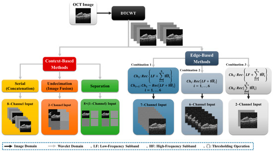
Figure 2.
General overview of the different subbands combination in the noisy and denoised conditions.
Two different types of subband combination were considered in these architectures: context-based combinations, and edge-based combinations.
2.3.2. Context-Based Combination
Image subbands are employed as input data in this type of image subbands combination. This strategy uses a variety of strategies, including:
- concatenation or serialization;
- undecimation;
- separation.
The input image for the serial or concatenation mode of DTCWT consists of eight channels of different subbands that are put alongside each other.
Undecimated DTCWT coefficients contain two different image channels with subbands placed next to each other, with the main image size. The input image of the undecimated DTCWT has two-channel images with a modified mask.
Another input shape is channel separation, which is applied to investigate the impact of each of the eight subbands on OCT input images. All images are similar to the input image size, and those are one-channel images.
2.3.3. Edge-Based Combination
Unlike the context-based combination, the Edge-based combination highlights the edges, to adapt the network for semantic segmentation tasks. This approach reconstructs subband images using a soft thresholding method [50,51], to reduce noise. Soft thresholding only applies to high-pass and band-pass subbands. This reconstruction approach takes into account the following new sorts of input images:
- Combination 1 is a seven-channel input including reconstruction of all subbands as channel 1 and channels 2 to 7, including subtraction of the first channel with the reconstruction of low-frequency subbands and each high-frequency subband;
- Combination 2 is a six-channel input that comes from the reconstruction of low-frequency subbands and each high-frequency subband;
- Combination 3 is a two-channel input consisting of the reconstruction of all subbands in channel 1 and all high-frequency subbands in channel 2.
An edge-based method architecture is shown on the right side of Figure 2. This architecture is also useful for noisy conditions, because it preserves edges. In this method, wavelet transform decomposes data as averaging filters, with others that produce details. If the details are small, they can be eliminated without significantly impacting the data set’s key aspects. Thresholding is the process of setting all high-frequency subband coefficients to less than a certain threshold to zero. These coefficients are employed in an inverse wavelet transformation. We used DTCWT as a wavelet transform and implemented it in the different subbands.
2.4. Deep Learning Architecture Methods
Unet is an architecture developed for biomedical image segmentation [52]. Different variants of Unet and other architectures networks have been proposed to improve the performance of classic methods. To discover the optimal baseline models, multiple Unet algorithms and other cutting-edge networks were used on the proposed dataset of this study. We compared Unet, Unet+++, R2 Unet, Trans-Unet, and Swin Unet, and another three methods with optimal hyperparameters, and found that Trans-Unet produced the best results among the many methods; due to that, in this section, we will only cover the Trans-Unet method. Figure 3 shows the structure proposed Trans-UNet network.
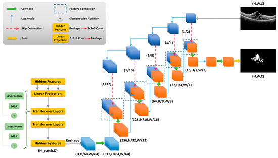
Figure 3.
Proposed Trans-Unet architecture for image segmentation.
2.4.1. Transformers
Transformers are novel structures that have been applied in various fields, such as natural language processing (NLP) [53], image segmentation [37], and image classification. This method tries to solve a problem through sequence-to-sequence tasks. This architecture solely depends on the self-attention mechanism. Trans-Unet is a deep learning segmentation algorithm that combines both transforms and Unet. The first part of the Trans-Unet is similar to the Conventional Unet. It extracts high-level features using convolutional layers, and it decodes in the last part; but using Trans-Unet, it applies a self-attention mechanism in the encoder part. In a Trans-Unet image with a size of , is the spatial resolution of the image and is the number of input channels; and this input is divided into embedding sequences [37].
2.4.2. Encoder
The proposed network is comprised of an encoder and decoders, as illustrated in Figure 3. Basic convolutional filter layers are implemented in the encoder section, followed by the ReLU activation map. Each input image is tokenized into flattened non-overlapping patches. The number of patches is calculated with the size of the patch ( with the length and sequence as input of the transformer.
To use the transformer layer to extract hidden features, vectorized image patches need to reshape it into a latent D-dimensional embedding space. This process is done using trainable linear projection. Patch spatial information is necessary for segmentation tasks that are encoded using position-embedding data. A trainable positional embedding layer is added to encode the patch spatial information. This layer holds the spatial information, which the transformer encoder layer has to model perfectly.
Equation (2) shows the initial value of the encoder, in which is the patch embedding projection, is the position embedding, and is the ith vectorized patch.
Each transformer encoder layer in Trans-Unet consists of the multihead self-attention (MSA) blocks and multi-layer perceptron (MLP) blocks. Equations (3) and (4) show how the MSA and MLP blocks are calculated for L layers.
In these equations, denotes the layer normalization operator. A residual connection is used to bypass each block, to build an identity map, and a layer normalization operator is placed in front of each block. The encoded image is finally obtained after iterative calculations of (3) and (4).
2.4.3. Decoder
As shown in Figure 3, the decoder tries to receive the abstract representation, which is similar to the Unet expanding part. The CNN decoder absorbs the transformer encoder’s feature maps and restores them to their original size. The decoder block starts with upsampling. An easy technique for segmentation is to simply upsample the encoded feature representation to full resolution, before predicting the dense output. The feature maps from the preceding layer are then concatenated using conventional convolution procedures. Up to this stage, it is similar to the Unet decoder. Here, to recover the spatial order, the size of the encoded feature should first be reshaped from to . Then, 1 × 1 convolution is applied to obtain a full-resolution image. The resulting tensor from the last layer is concatenated with the extracted transformer feature maps to enrich features. A one-dimensional predicted mask results from fusing the last layer result in the last stage.
2.4.4. Loss Function
OCT images are unbalanced, which means the fluid ratio is much higher than the non-fluid part in the gold standard mask [54]. One of the most difficult aspects of the OCT fluid segmentation process is dealing with imbalanced data. One of the options to handle imbalanced data is using the Dice score coefficient (DSC) as a loss function. Tversky loss is offered as a replacement for the Dice coefficient, which equally considers false negatives (FNs) and false positives (FPs) [55].
The Tversky index (TI) is an asymmetric similarity measure that combines the Dice coefficient, and it is calculated as below:
The has two additional parameters, , where . In the case of , it is reduced to the Dice coefficient.
2.4.5. Metrics
Dice Coefficient
The Dice coefficient or f1-score represents the basic similarity between images’ predicted masks and grand truth masks. It calculates the overlap between the and images, one as a predicted image and the other as a true mask. The formula is defined as follows:
Jaccard Index
The Jaccard similarity index is similar to the Dice coefficient. It compares members for two sets and calculates the similarities between sample sets. and are similar to the Dice definition. One of them is the predicted image, and the other one is the true mask It is defined as in the below formula:
3. Results
The proposed methods for fluid segmentation were combined with different subband architectures to segment all pixels in each B-scan into IRF, SRF, PED, and tissue. In the first step, different Unet model techniques and other cutting-edge methods were applied for OCT semantic segmentation, to select the Unet base model for subband comparisons. Various subbands with different input channels and types were investigated in this study. Dice coefficients and the Jaccard metrics for semantic segmentation tasks were employed as assessment metrics. Furthermore, we analyzed the visualization results of the different subbands. For a fair comparison, we implemented a fixed 150 epochs for Unet selection and subband compressions, and this number was selected based on the available results.
A brief description of each approach’s results is given below:
- Different types of cutting-edge semantic segmentation network, such as Unet, Attention Unet, Unet+++, R2 Unet, Trans-Unet, and Swin Unet with best-fit parameters, and three other completely different models for this application were implemented;
- The DTCWT extracted subbands with various architectures were applied to analyze the best subband combinations;
- Each subband was tested separately, to find the best results among all subband images.
We also investigated subbands in a noisy environment using different subband formations with denoised reconstruction, to perform fluid area segmentation in the noisy condition and to assess the efficacy of the suggested approaches, which will be discussed later in the experiment section.
3.1. Unet Selection
For the localization of fluid in DME and AMD patients, we examined the performance of multiple state-of-the-art Unets for fluid segmentation techniques. In addition to networks, three alternative network models with superior performance were employed for comparison [28,32,34]. First, we undertook a quantitative study of the segmentation findings on images from two datasets (OPTIMA and our dataset). The segmentation results are given in Figure 4. We adopted the K-fold cross-validation (K = 5) procedure, in which we employed four sets (4400 images with an augmentation process) of five images as the training set and one set (1100 images) as the test set.
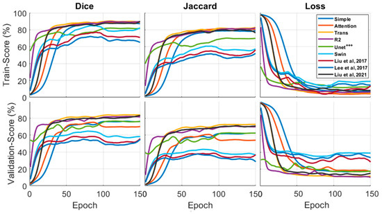
Figure 4.
The Dice, Jaccard, and loss curves were used to compare the different models. All of the models performed well in the metrics comparison. The best Dice and Jaccard results were obtained by Trans-Unet models, with 90.7 and 82.1 validation, while Swin Unet produced the worst results.
The quantitative results of the segmentation after applying hyperparameter optimization of the proposed networks on images from nine networks are shown in Figure 5. While Table 1 illustrates the results of different models using Jaccard and Dice outcomes.
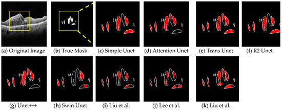
Figure 5.
Comparison of segmentation results of the different Unet experiments on the B-Scan. (a) the original image. (b) True Mask. (c) Simple Unet. (d) Attention Unet. (e) Trans-Unet. (f) R2 Unet. (g) Unet+++. (h) Swin Unet. (i–k) Different state of the arts network structures [28,32,34]. Segmentations contain a white boundary that compares the extracted result with the true mask.

Table 1.
Five-fold cross-validation score of all Unet models after applying hyperparameter optimization.
The first and second columns in Figure 4 show the Dice and Jaccard outcomes of the various networks. The loss function results are in the third column. As seen in the diagram, the trans-Unet technique had the best performance compared to the other Unets and cutting-edge networks. The Trans-Unet with the parameters in Table 2 had a superior validation outcome to the other networks with the same filter sizes.
Table 2.
Trans-Unet network parameters.
Figure 5 shows the qualitative results of the networks with fluid, the ground-truth annotations (second column), and the segmentation results of each network in further cells. As seen in the figure, the Trans-Unet approach had the best performance for both closed and large fluid areas. Due to these results, we chose Trans-Unet with the optimum parameters for the basic network for analyzing the subband inputs.
3.2. Input Image Transformations
As previously stated, this study considered two distinct subband combinations: context-based, and edge-based. In the concatenating wavelet, subbands of images are combinations that put images alongside each other. This structure examines the influence of subbands when they are concatenated with each other. In DTCWT, all subbands are employed in this type of combination.
Channel separation results are another type of context-based solution to the fluid segmentation problem. The task of separating an image into its different subband contents is beneficial for analyzing the effect of each subband. We chose the best separation results between the various subband combinations. In Figure 6, a boxplot of the sensitivity and false positive ratio (FPR) of each subband is shown, using this formula:
where is similar to Equation (5) (true positive), and is (false positive) is the number of pixels that are correctly and incorrectly predicted as tumor pixels in the image, respectively. In addition, is the number of actual tumor pixels in the image, and is the total number of non-tumor pixels. The L1 and L2 subbands performed better than the other subbands. We chose the L1 subband because it had a high sensitivity and less FPR than the other methods.
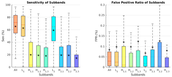
Figure 6.
Boxplot of the comparative analysis between the different subband segmentation separation results for the test data set. (Left panel): Sensitivity. (Right panel): False positive ratio. The star (*) in each box is the mean score. The line represents the median scores.
Undecimated wavelet transform combination methods demonstrate the importance of subbands in a single image and are also a novel formation that can be applied and fused. In an undecimated combination, we need different loss functions because of the changing masks. Therefore, our problem has slightly changed. Previously, we had unbalanced tasks. Our problem has changed to a more balanced condition, by changing the masks. Thus, the loss function was changed, to collect the best results for this type. The focal Tversky loss function with the following formula was applied for this reason [56]:
In Figure 7, the first column is the Dice results, the second column is the Jaccard results, and the third column is the loss function results, based on a fixed 150 epochs. Figure 8 shows the concatenation, and the best separation subband produced a better result than a simple image. In these results, we examined different methods alongside each other. These results were context-based and had a good performance when comparing simple images.
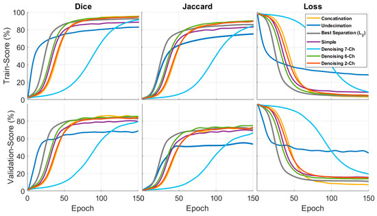
Figure 7.
Quantitative results for the Dice, Jaccard, and loss functions of the proposed input architectures. The first and second columns indicate the Dice and Jaccard scores on the training and test datasets. The third column illustrates the loss function curve.
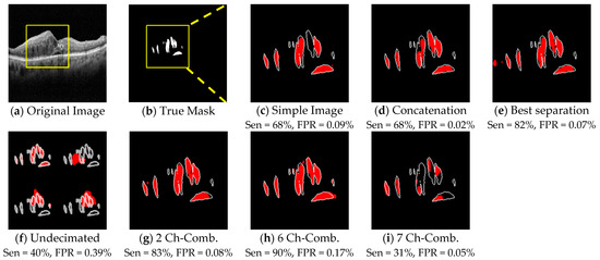
Figure 8.
Comparison of different method segmentation results. (a) Original image, (b) a true mask from experts, and (c) the result of a simple image extracted using trans-Unet. (d~f) Segmentation results of the different proposed context-based method combinations. (g~i) segmentation results of the edge-based method combinations.
Another type of method compared in this figure is the edge-based technique. We tried to highlight edges in three novel ways with edge-based techniques.
There are a variety of denoising approaches that can be employed in the reconstruction of OCT images. For noise reduction in OCT images, a soft threshold-based denoising methodology is used [56]. The extracted combination subbands for DTCWT that were explained in the material and method section are as follows:
- two-channel;
- six-channel;
- seven-channel.
A comparison of edge-based techniques with simple and context-based images is given in Figure 7. As can be seen, the edge-based methods outperformed the others, particularly in terms of their quicker convergence. The convergence speed and outcomes of the two-channel edge-based approach were satisfactory. The rationale for the improved performance of the edge-based approaches over the simple images is that edge-based combination edges are highlighted, allowing the network to execute semantic segmentation more easily.
Table 3 displays the quantitative results for Dice and Jaccard for the various combinations. The excellent impact of the DTCWT subbands in comparison to the simple image is exhibited in this table. These combinations allowed improvement of the semantic segmentation outcomes. Edge-based combinations had better results than context-based ones. The six-channel edge-based combination had better results than the others. The quantitative results of the different methods are demonstrated in Figure 8, illustrating the excellent effect of the subbands used in DTCWT. The qualitative results proved that subbands could extract better boundaries for a sample image. The sensitivity and FPR were calculated for each subband. According to Table 3 and Figure 8, the two-channel and six-channel edge-based techniques had a better performance than the others.
Table 3.
Comparison of the different individual DTCWT subbands in the proposed dataset.
The results for varying numbers of input transforms are shown in Figure 9. This figure allows a numeric analysis based on the qualitative results. As can be seen, edge-based six- and two-channel techniques had a high sensitivity and lower amount of FPR.
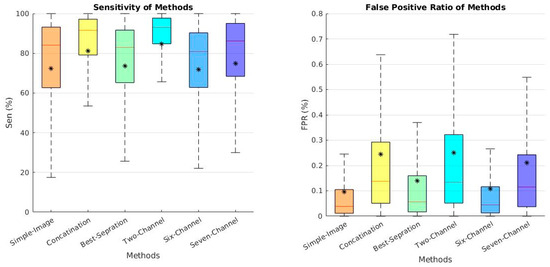
Figure 9.
Boxplot of a comparative analysis between the different inputs for transformation segmentation. The star (*) in each box is the mean score.
3.3. Results of Noise Adding
Although our dataset contained Heidelberg images with a low noise level, some of the OCT modalities contain a high noise level, and our method needed to be tested on noisy conditions. Therefore, we added Gaussian noise and denoised images and subbands to evaluate the subbands’ behavior in a noisy environment.
Gaussian noise with different standard deviations was added to the image in the pixel domain, to create a new dataset with which to test the robustness of the proposed method. A variety of denoising approaches can be employed in OCT images. For noise reduction in OCT images, we used the soft thresholding denoising methodology in the DTCWT domain [57]. Two standard deviations of 80 and 160 were added to images in the noisy condition, to test the robustness of using the different inputs. The main goal of this experiment was to evaluate the OCT fluid segmentation results in the noise-added conditions; in this regard, we implemented edge-based combinations. Edge-based approaches attempt to emphasize edges and perform well in noisy environments.
Figure 10 and Figure 11 show the Dice and Jaccard of the train and validation results. This experiment was similar to the other parts we compared with Dice, Jaccard, and loss graphs. The edge-based methods had a significant result, especially in the validation index. In addition, as can be deduced from Figure 10 and Figure 11, the six-channel results had a better performance in both noise-added conditions.
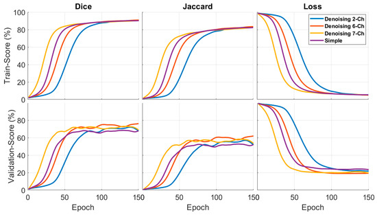
Figure 10.
Effect of added noised on the segmentation Dice and Jaccard, σ = 80. The results were obtained using edge-based methods.
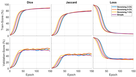
Figure 11.
Effect of added noised on the segmentation Dice and Jaccard, high level of noise (σ = 160). The results were obtained using edge-based methods.
Table 4 reports the values of the different methods: the subband combination results were similar and they performed significantly better than a simple image. The six-channel and two-channel results were comparable and exceeded the others.
Table 4.
Summarized performance with different levels of noise added after denoising and reconstruction.
The sensitivity and FPR performance the of edge-based methods in noised added conditions is presented in Figure 12. The six-channel method exhibited a good sensitivity and a decreased FPR with high noise levels, as illustrated in Figure 12. The two-channel findings were quite similar to the six-channel results. These graphs demonstrate that the edge-based methods provided a superior visualization over the simple images.
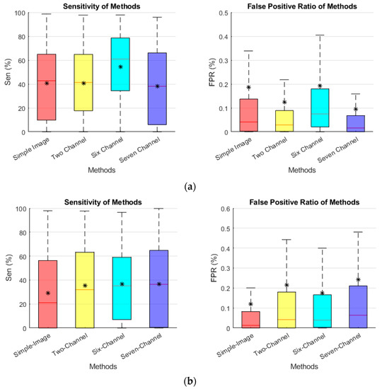
Figure 12.
Effect of added noised on the segmentation sensitivity and FPR. (a) σ = 80. (b) σ = 160. The star (*) in each box is the mean score.
Finally, Figure 13 illustrates the qualitative results. The subband combinations could persevere the edges in noisy image segmentation, and the subband combination images extracted the boundaries and fluid sections better than the simple images.
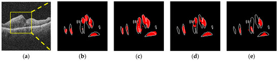
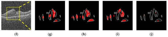
Figure 13.
Sample image for different noise-added conditions (noise 80 and 160). The first row is with a noise level of 80, and the second row is the result of the 160 noise level. (a) σ = 80. (b) 2 Ch-Comb. Sen = 44%, FPR = 0.15%. (c) 6 Ch-Comb. Sen = 73%, FPR = 0.25%. (d) 7 Ch-Comb. Sen = 48%, FPR = 0.09%. (e) Simple image. Sen = 31%, FPR = 0.04%. (f) σ = 160. (g) 2 Ch-Comb. Sen = 33%, FPR = 0.12%. (h) 6 Ch-Comb. Sen = 47%, FPR = 0.19%. (i) 7 Ch-Comb. Sen = 38%, FPR = 0.19%. (j) Simple image. Sen = 3%, FPR = 0%.
4. Discussion
We suggested subband-based DTCWT fluid segmentation approaches based on deep learning transformers. We used numerous measures and strategies to evaluate the performance of the proposed inputs and subbands. The optimum network for OCT segmentation was chosen in this procedure. As illustrated in Figure 2, context-based and edge-based methods were suggested for the input transform. The DTCWT subband combination approach produced the best comparative results when selecting the best combination. Our technique and some of the diverse inputs resulted in better Dice and Jaccard results in the quantitative analysis and a faster loss reduction. The visualization results analysis revealed considerable improvements for the various subband formations. In addition, the FPR and sensitivity of the various methods were calculated, to compare the performance of the methods in the visualization. The performance of pairs that emphasized edges (edge-based methods) outperformed the context-based techniques. The six-channel and two-channel edge-based methods produced the best input for OCT cyst segmentation.
The findings in the different figures reveal that applying subbands in the different methods was more suitable for closely segmenting the fluid regions. This allowed separating the independent regions more precisely. Furthermore, it was demonstrated that employing subbands under noise-added situations was effective. We conducted tests to compare the influence of images under noise-added conditions with various noise intensity parameters. It was discovered that the applied subband outperformed the simple image for edge-based methods. The robustness of the suggested strategy was demonstrated by the findings shown in Figure 11 and Figure 12. We also investigated the performance of each subband and analyzed the performance of each subband for low-pass and high-pass filters. The results indicated that each subband could add more information to the main image.
5. Conclusions and Future Work
Segmenting fluid areas in retinal OCT images is very important, since it may help the clinician detect macular edema and conduct treatment procedures promptly. This paper proposed an automatic fluid segmentation method in retinal OCT images using DTCWT subband combinations based on deep learning. The study’s main purpose was to examine the performance of DTCWT in semantic segmentation of normal and noisy images of OCT corrupted by different noise levels.
Network and different input approaches were considered. A novel U-net algorithm for OCT segmentation was applied as the base of the network. To exploit a U-net based on transformers, different wavelet-based subband combinations were constructed.
We introduced different subband formations, context-based and Edge-based, as the input transforms to properly segment fluid regions in OCT images. We also analyzed each combination, to find the best subbands that could process the main images for segmentation. The proposed methods showed very promising segmentation performances, and which were competitive with the state-of-the-art alternatives.
The results showed that the DTCWT subband combinations in the proposed U-net yielded better semantic segmentation results for both datasets. The enhanced performance was due to the subbands’ capacity to capture the directional properties of linear and nonlinear discontinuities. The six-channel and two-channel edge-based techniques had the best performance among the other input transform shapes.
A variety of future tasks must be completed. For instance, one planned future work includes fine-tuning the parameters and incorporating a loss function and a model hyperparameter. Future work will include using other X-lets, selecting the optimal combination among them, and introducing a unique loss function, and this will be published shortly. This loss function could be used to analyze subbands as a network loss function, and also a novel U-net architecture based on subbands will be proposed. Another idea we will investigate in the future is applying different X-let subbands, using a mixture of experts.
Author Contributions
Conceptualization, R.K. and H.R.; methodology, R.D., R.K. and H.R.; software, R.D. and M.N.; validation, R.D., R.K. and H.R.; formal analysis, R.D. and M.N.; investigation, R.D.; resources, H.R.; data curation, R.D. and M.N.; writing—original draft preparation, R.D., M.N., R.K. and H.R.; writing—review and editing, R.D., R.K. and H.R.; visualization, R.D. and M.N.; supervision, H.R.; project administration, H.R.; funding acquisition, H.R. All authors have read and agreed to the published version of the manuscript.
Funding
This research received no external funding.
Institutional Review Board Statement
Not applicable.
Informed Consent Statement
Not applicable.
Data Availability Statement
Not applicable.
Acknowledgments
We sincerely appreciate all valuable comments and suggestions of Gerlind Plonka, which helped us to improve the quality of the article.
Conflicts of Interest
The authors declare no conflict of interest.
References
- Roglic, G. WHO Global report on diabetes: A summary. Int. J. Noncommun. Dis. 2016, 1, 3–8. [Google Scholar] [CrossRef]
- Ciulla, T.A.; Amador, A.G.; Zinman, B. Diabetic retinopathy and diabetic macular edema: Pathophysiology, screening, and novel therapies. Diabetes Care 2003, 26, 2653–2664. [Google Scholar] [CrossRef] [PubMed]
- de Jong, E.; Geerlings, M.; den Hollander, A. Chapter 10-Age-Related Macular Degeneration; Academic Press: Cambridge, MA, USA; pp. 155–180.
- Wang, Y.; Zhang, Y.; Yao, Z.; Zhao, R.; Zhou, F. Machine learning based detection of age-related macular degeneration (AMD) and diabetic macular edema (DME) from optical coherence tomography (OCT) images. Biomed. Opt. Express 2016, 7, 4928–4940. [Google Scholar] [PubMed]
- Bhagat, N.; Grigorian, R.A.; Tutela, A.; Zarbin, M.A. Diabetic macular edema: Pathogenesis and treatment. Surv. Ophthalmol. 2009, 54, 1–32. [Google Scholar] [PubMed]
- Kaymak, S.; Serener, A. Automated age-related macular degeneration and diabetic macular edema detection on oct images using deep learning. In Proceedings of the 2018 IEEE 14th International Conference on Intelligent Computer Communication and Processing (ICCP), Cluj-Napoca, Romania, 6–8 September 2018; IEEE: Piscataway, NJ, USA, 2018. [Google Scholar]
- Panozzo, G.; Gusson, A.; Parolini, B.; Mercanti, A. Role of OCT in the diagnosis and follow up of diabetic macular edema. in Seminars in ophthalmology. Semin Ophthalmol. 2003, 18, 74–81. [Google Scholar]
- Alsaih, K.; Lemaitre, G.; Rastgoo, M.; Massich, J.; Sidibé, D.; Meriaudeau, F. Machine learning techniques for diabetic macular edema (DME) classification on SD-OCT images. Biomed. Eng. Online 2017, 16, 68. [Google Scholar]
- Parhi, K.K.; Rashno, A.; Nazari, B.; Sadri, S.; Rabbani, H.; Drayna, P.; Koozekanani, D.D. Automated fluid/cyst segmentation: A quantitative assessment of diabetic macular edema. Investig. Ophthalmol. Vis. Sci. 2017, 58, 4633. [Google Scholar]
- Rashno, A.; Koozekanani, D.D.; Drayna, P.M.; Nazari, B.; Sadri, S.; Rabbani, H.; Parhi, K.K. Fully automated segmentation of fluid/cyst regions in optical coherence tomography images with diabetic macular edema using neutrosophic sets and graph algorithms. IEEE Trans. Biomed. Eng. 2017, 65, 989–1001. [Google Scholar] [CrossRef]
- Schlegl, T.; Waldstein, S.M.; Bogunovic, H.; Endstraßer, F.; Sadeghipour, A.; Philip, A.M.; Podkowinski, D.; Gerendas, B.S.; Langs, G.; Schmidt-Erfurth, U. Fully automated detection and quantification of macular fluid in OCT using deep learning. Ophthalmology 2018, 125, 549–558. [Google Scholar] [CrossRef]
- Garcia-Garcia, A.; Orts-Escolano, S.; Oprea, S.; Villena-Martinez, V.; Garcia-Rodriguez, J. A review on deep learning techniques applied to semantic segmentation. arXiv 2017, arXiv:1704.06857. [Google Scholar]
- Lateef, F.; Ruichek, Y. Survey on semantic segmentation using deep learning techniques. Neurocomputing 2019, 338, 321–348. [Google Scholar] [CrossRef]
- Alsaih, K.; Yusoff, M.Z.; Tang, T.B.; Faye, I.; Mériaudeau, F. Deep learning architectures analysis for age-related macular degeneration segmentation on optical coherence tomography scans. Comput. Methods Programs Biomed. 2020, 195, 105566. [Google Scholar] [CrossRef]
- Hao, S.; Zhou, Y.; Guo, Y. A brief survey on semantic segmentation with deep learning. Neurocomputing 2020, 406, 302–321. [Google Scholar] [CrossRef]
- Ulku, I.; Akagündüz, E. A survey on deep learning-based architectures for semantic segmentation on 2d images. Appl. Artif. Intell. 2022, 36, 2032924. [Google Scholar] [CrossRef]
- Garcia-Garcia, A.; Orts-Escolano, S.; Oprea, S.; Villena-Martinez, V.; Martinez-Gonzalez, P.; Garcia-Rodriguez, J. A survey on deep learning techniques for image and video semantic segmentation. Appl. Soft Comput. 2018, 70, 41–65. [Google Scholar] [CrossRef]
- Ansari, R.A.; Malhotra, R.; Buddhiraju, K.M. Identifying Informal Settlements Using Contourlet Assisted Deep Learning. Sensors 2020, 20, 2733. [Google Scholar] [CrossRef]
- Lin, M.; Bao, G.; Sang, X.; Wu, Y. Recent Advanced Deep Learning Architectures for Retinal Fluid Segmentation on Optical Coherence Tomography Images. Sensors 2022, 22, 3055. [Google Scholar] [CrossRef]
- Chen, Z.; Li, D.; Shen, H.; Mo, H.; Zeng, Z.; Wei, H. Automated segmentation of fluid regions in optical coherence tomography B-scan images of age-related macular degeneration. Opt. Laser Technol. 2020, 122, 105830. [Google Scholar] [CrossRef]
- Ciresan, D.; Giusti, A.; Gambardella, L.; Schmidhuber, J. Deep neural networks segment neuronal membranes in electron microscopy images. In Proceedings of the Advances in Neural Information Processing Systems, Lake Tahoe, NV, USA, 3–6 December 2012; 2012; Volume 25. [Google Scholar]
- Hariharan, B.; Arbeláez, P.; Girshick, R.; Malik, J. Simultaneous detection and segmentation. In Proceedings of the European Conference on Computer Vision, Zurich, Switzerland, 6–12 September 2014; Springer: New York, NY, USA, 2014. [Google Scholar]
- Mo, Y.; Wu, Y.; Yang, X.; Liu, F.; Liao, Y. Review the state-of-the-art technologies of semantic segmentation based on deep learning. Neurocomputing 2022, 493, 626–646. [Google Scholar] [CrossRef]
- Long, J.; Shelhamer, E.; Darrell, T. Fully convolutional networks for semantic segmentation. In Proceedings of the IEEE Conference on Computer Vision and Pattern Recognition, Boston, MA, USA, 7–12 June 2015. [Google Scholar]
- Oktay, O.; Schlemper, J.; Folgoc, L.L.; Lee, M.; Heinrich, M.; Misawa, K.; Mori, K.; McDonagh, S.; Hammerla, N.Y.; Kainz, B.; et al. Attention u-net: Learning where to look for the pancreas. arXiv 2018, arXiv:1804.03999. [Google Scholar]
- Chen, L.C.; Zhu, Y.; Papandreou, G.; Schroff, F.; Adam, H. Encoder-decoder with atrous separable convolution for semantic image segmentation. In Proceedings of the European Conference on Computer Vision (ECCV), Munich, Germany, 8–14 September 2018. [Google Scholar]
- Optima Cyst Segmentation Challenge. 2015. Available online: https://optima.meduniwien.ac.at/research/challenges/ (accessed on 5 October 2015).
- Liu, D.; Liu, X.; Fu, T.; Yang, Z. Fluid region segmentation in OCT images based on convolution neural network. In Proceedings of the Ninth International Conference on Digital Image Processing (ICDIP 2017), Hong Kong, China, 19–22 May 2017; SPIE: Bellingham, WA, USA, 2017. [Google Scholar]
- Roy, A.G.; Conjeti, S.; Karri SP, K.; Sheet, D.; Katouzian, A.; Wachinger, C.; Navab, N. ReLayNet: Retinal layer and fluid segmentation of macular optical coherence tomography using fully convolutional networks. Biomed. Opt. Express 2017, 8, 3627–3642. [Google Scholar] [CrossRef] [PubMed]
- Morley, D.; Foroosh, H.; Shaikh, S.; Bagci, U. Simultaneous detection and quantification of retinal fluid with deep learning. arXiv 2017, arXiv:1708.05464. [Google Scholar]
- Tennakoon, R.; Gostar, A.K.; Hoseinnezhad, R.; Bab-Hadiashar, A. Retinal fluid segmentation and classification in OCT images using adversarial loss based CNN. In Proceedings of the 2018 IEEE 15th International Symposium on Biomedical Imaging (ISBI 2018), Washington DC, USA, 4–7 April 2018; pp. 30–37. [Google Scholar]
- Lee, C.S.; Tyring, A.J.; Deruyter, N.P.; Wu, Y.; Rokem, A.; Lee, A.Y. Deep-learning based, automated segmentation of macular edema in optical coherence tomography. Biomed. Opt. Express 2017, 8, 3440–3448. [Google Scholar] [CrossRef] [PubMed]
- Gopinath, K.; Sivaswamy, J. Segmentation of retinal cysts from optical coherence tomography volumes via selective enhancement. IEEE J. Biomed. Health Inform. 2018, 23, 273–282. [Google Scholar] [CrossRef] [PubMed]
- Liu, X.; Wang, S.; Zhang, Y.; Liu, D.; Hu, W. Automatic fluid segmentation in retinal optical coherence tomography images using attention based deep learning. Neurocomputing 2021, 452, 576–591. [Google Scholar] [CrossRef]
- Huang, H.; Lin, L.; Tong, R.; Hu, H.; Zhang, Q.; Iwamoto, Y.; Han, X.; Chen, Y.W.; Wu, J. Unet 3+: A full-scale connected unet for medical image segmentation. In Proceedings of the ICASSP 2020-2020 IEEE International Conference on Acoustics, Speech and Signal Processing (ICASSP), Barcelona, Spain, 4–8 May 2020; IEEE: Piscataway, NJ, USA, 2020. [Google Scholar]
- Alom, M.Z.; Hasan, M.; Yakopcic, C.; Taha, T.M.; Asari, V.K. Recurrent residual convolutional neural network based on u-net (r2u-net) for medical image segmentation. arXiv 2018, arXiv:1802.06955. [Google Scholar]
- Chen, J.; Lu, Y.; Yu, Q.; Luo, X.; Adeli, E.; Wang, Y.; Lu, L.; Yuille, A.L.; Zhou, Y. Transunet: Transformers make strong encoders for medical image segmentation. arXiv 2021, arXiv:2102.04306. [Google Scholar]
- Cao, H.; Wang, Y.; Chen, J.; Jiang, D.; Zhang, X.; Tian, Q.; Wang, M. Swin-unet: Unet-like pure transformer for medical image segmentation. arXiv 2021, arXiv:2105.05537. [Google Scholar]
- Addison, P.S.; Walker, J.; Guido, R.C. Time--frequency analysis of biosignals. IEEE Eng. Med. Biol. Mag. 2009, 28, 14–29. [Google Scholar] [CrossRef]
- Lu, H.; Wang, H.; Zhang, Q.; Won, D.; Yoon, S.W. A dual-tree complex wavelet transform based convolutional neural network for human thyroid medical image segmentation. In Proceedings of the 2018 IEEE International Conference on Healthcare Informatics (ICHI), New York, NY, USA, 4–7 June 2018; IEEE: Piscataway, NJ, USA, 2018. [Google Scholar]
- Li, Q.; Shen, L. Wavesnet: Wavelet integrated deep networks for image segmentation. arXiv 2020, arXiv:2005.14461. [Google Scholar]
- Zhang, R. Making Convolutional Networks Shift-Invariant Again. In Proceedings of the 36th International Conference on Machine Learning, Long Beach, CA, USA, 9–15 June 2019; Kamalika, C., Ruslan, S., Eds.; PMLR: Proceedings of Machine Learning Research. pp. 7324–7334. [Google Scholar]
- de Souza Brito, A.; Vieira, M.B.; de Andrade ML, S.C.; Feitosa, R.Q.; Giraldi, G.A. Combining max-pooling and wavelet pooling strategies for semantic image segmentation. Expert Syst. Appl. 2021, 183, 115403. [Google Scholar] [CrossRef]
- Alijamaat, A.; NikravanShalmani, A.R.; Bayat, P. Diagnosis of Multiple Sclerosis Disease in Brain MRI Images using Convolutional Neural Networks based on Wavelet Pooling. J. AI Data Min. 2021, 9, 161–168. [Google Scholar]
- Alijamaat, A.; NikravanShalmani, A.; Bayat, P. Multiple sclerosis identification in brain MRI images using wavelet convolutional neural networks. Int. J. Imaging Syst. Technol. 2021, 31, 778–785. [Google Scholar] [CrossRef]
- Yang, G.; Geng, P.; Ma, H.; Liu, J.; Luo, J. DWTA-Unet: Concrete Crack Segmentation Based on Discrete Wavelet Transform and Unet. In Proceedings of the 2021 Chinese Intelligent Automation Conference, Zhanjiang, China, 5–7 November 2021; Springer: New York, NY, USA, 2021. [Google Scholar]
- Zhang, Y.; Wang, C.; Ji, Y.; Chen, J.; Deng, Y.; Chen, J.; Jie, Y. Combining segmentation network and nonsubsampled contourlet transform for automatic marine raft aquaculture area extraction from sentinel-1 images. Remote Sens. 2020, 12, 4182. [Google Scholar] [CrossRef]
- Bi, H.; Xu, L.; Cao, X.; Xue, Y.; Xu, Z. Polarimetric SAR image semantic segmentation with 3D discrete wavelet transform and Markov random field. IEEE Trans. Image Process. 2020, 29, 6601–6614. [Google Scholar] [CrossRef]
- Montazerin, M.; Sajjadifar, Z.; Khalili Pour, E.; Riazi-Esfahani, H.; Mahmoudi, T.; Rabbani, H.; Movahedian, H.; Dehghani, A.; Akhlaghi, M.; Kafieh, R. Livelayer: A semi-automatic software program for segmentation of layers and diabetic macular edema in optical coherence tomography images. Sci. Rep. 2021, 11, 13794. [Google Scholar] [CrossRef]
- Selesnick, I.W.; Baraniuk, R.G.; Kingsbury, N.C. The dual-tree complex wavelet transform. IEEE Signal Process. Mag. 2005, 22, 123–151. [Google Scholar] [CrossRef]
- Chitchian, S.; Fiddy, M.A.; Fried, N.M. Denoising during optical coherence tomography of the prostate nerves via wavelet shrinkage using dual-tree complex wavelet transform. J. Biomed. Opt. 2009, 14, 014031. [Google Scholar] [CrossRef]
- Ronneberger, O.; Fischer, P.; Brox, T. U-net: Convolutional networks for biomedical image segmentation. In Proceedings of the International Conference on Medical Image Computing and Computer-Assisted Intervention, Munich, Germany, 5–9 October 2015; Springer: New York, NY, USA, 2015. [Google Scholar]
- Otter, D.W.; Medina, J.R.; Kalita, J.K. A survey of the usages of deep learning for natural language processing. IEEE Trans. Neural Netw. Learn. Syst. 2020, 32, 604–624. [Google Scholar] [CrossRef]
- Oguz, I.; Zhang, L.; Abràmoff, M.D.; Sonka, M. Optimal retinal cyst segmentation from OCT images. In Proceedings of the Medical Imaging 2016: Image Processing, San Diego, CA, USA, 10 January 2016; International Society for Optics and Photonics: Bellingham, WA, USA, 2016. [Google Scholar]
- Sudre, C.H.; Li, W.; Vercauteren, T.; Ourselin, S.; Jorge Cardoso, M. Generalised dice overlap as a deep learning loss function for highly unbalanced segmentations. In Deep Learning in Medical Image Analysis and Multimodal Learning for Clinical Decision Support; Springer: New York, NY, USA, 2017; pp. 240–248. [Google Scholar]
- Abraham, N.; Khan, N.M. A novel focal tversky loss function with improved attention u-net for lesion segmentation. In Proceedings of the 2019 IEEE 16th International Symposium on Biomedical Imaging (ISBI 2019), Venezia, Italy, 8–11 April 2019; IEEE: Piscataway, NJ, USA, 2019. [Google Scholar]
- Sendur, L.; Selesnick, I.W. Bivariate shrinkage functions for wavelet-based denoising exploiting interscale dependency. IEEE Trans. Signal Process. 2002, 50, 2744–2756. [Google Scholar] [CrossRef]
Disclaimer/Publisher’s Note: The statements, opinions and data contained in all publications are solely those of the individual author(s) and contributor(s) and not of MDPI and/or the editor(s). MDPI and/or the editor(s) disclaim responsibility for any injury to people or property resulting from any ideas, methods, instructions or products referred to in the content. |
© 2022 by the authors. Licensee MDPI, Basel, Switzerland. This article is an open access article distributed under the terms and conditions of the Creative Commons Attribution (CC BY) license (https://creativecommons.org/licenses/by/4.0/).