
Article

Decadal Shifts in Zooplankton Size Structure and Biomass in a Warming Tropical Lake
1
Department of Fisheries and Water Resources, University of Energy and Natural Resources, Sunyani P.O. Box 214, Ghana
2
Department of Ecology, Faculty of Humanities and Natural Sciences, University of Presov, 17. novembra 1, 080 01 Prešov, Slovakia
3
Department of Environmental Management, University of Energy and Natural Resources, Sunyani P.O. Box 214, Ghana
*
Authors to whom correspondence should be addressed.
Limnol. Rev. 2026, 26(3), 47; https://doi.org/10.3390/limnolrev26030047
Submission received: 24 April 2026 / Revised: 24 July 2026 / Accepted: 5 August 2026 / Published: 10 August 2026
(This article belongs to the Topic Water Management in the Age of Climate Change)

Abstract

Climate warming can alter lake zooplankton through changes in thermal structure, oxygen availability, nutrient cycling, and phytoplankton dynamics, but decadal evidence from African lakes remains scarce. We compared zooplankton size structure and biomass in Lake Bosumtwi, Ghana, between 2005–2006 and 2018–2020, using harmonised historical data and recent observations of zooplankton, temperature, dissolved oxygen, nutrients, chlorophyll a, and water transparency. Water temperatures increased across all depth strata, with the largest increase in the epilimnion (+0.30 °C), while dissolved oxygen declined by approximately 27%. Epilimnetic total nitrogen, total phosphorus, and chlorophyll a increased, and water transparency decreased. Chlorophyll a rose by 142% between periods, while mean total zooplankton biomass increased 2.33-fold, mainly because of higher copepod biomass. Mean body length decreased in nauplii but increased in copepodites and adult copepods, indicating contrasting stage-specific shifts in size structure. The median zooplankton biomass-to-chlorophyll a ratio increased from 59.46 to 79.24 (Mann–Whitney U = 210, p = 0.032). Biomass differed significantly among years for copepods, rotifers, and total zooplankton, but not for cladocerans. These findings show that warmer and less oxygenated conditions with higher chlorophyll a concentrations were accompanied by a substantial increase in copepod-dominated biomass and stage-specific changes in zooplankton size structure.

1. Introduction

Zooplankton dynamics in lakes are regulated by a complex array of biological, environmental, climatic, and anthropogenic factors such as nutrient enrichment, climate warming, land use change, hydrological variability, and trophic interactions. These drivers also affect long-term shifts in abundance, biomass, and community structure [1,2,3,4]. Nutrient loading and eutrophication stimulate phytoplankton production, reducing zooplankton species richness and diversity [3]. Hydrodynamic changes, such as wind-driven mixing, affect vertical migration and reproduction, while top-down (e.g., predation) and bottom-up (e.g., food availability) forces regulate zooplankton biomass [2]. Lake temperatures have risen globally, with an average warming rate of approximately 0.34 °C per decade reported for 1985–2009 [5,6,7,8]. Continued warming is expected to alter thermal structure, biotic community structure, and food-web functioning in aquatic ecosystems [9,10,11,12,13]. Warming can alter zooplankton body size, phenology, survival, development, and metabolic demand, although responses vary among taxa and ecosystems [14,15,16,17,18,19,20,21,22,23]. For example, cyclopoid copepods of the genus Mesocyclops are trophically flexible omnivores that can exploit suitable phytoplankton, ciliates, rotifers, and small cladocerans, allowing them to respond to changes in both basal resources and the availability of animal prey [24,25,26].
In many tropical lakes, climate warming has intensified stratification, prolonged thermal stability, reduced mixing depth, altered vertical nutrient transport, and modified the oxygenated habitat [27,28,29]. Climate change alters the structure and functioning of tropical lakes [30], with increased epilimnetic temperatures promoting persistent stratification and reduced seasonal mixing depths [27,31], thereby affecting nutrient cycling, primary productivity, and zooplankton communities. Sharp density gradients in warm waters make tropical lakes particularly prone to intensified stratification and warming [8,32]. Thermoclines in deep tropical African lakes also fluctuate widely with climate variability within a narrow but high temperature range [33]. Declines in primary productivity have been linked to prolonged stratification and nutrient accumulation in deep waters under warming conditions [28,34]. Warmer lake temperatures can alter habitat conditions and affect lake biota [35], including zooplankton [23], through cumulative physiological and ecological stressors [11] that may reduce reproductive success [36].
Evidence from marine, temperate freshwater, and tropical freshwater ecosystems indicates that climate-related environmental change can substantially alter zooplankton biomass, although the direction and magnitude of responses vary among ecosystems, taxa, and functional groups [23,37]. Model projections suggest that future reductions in phytoplankton biomass could cause corresponding declines in zooplankton, with unequal effects among functional groups [37]. Warming and increased water-column stability may also alter phytoplankton composition and favour less palatable taxa, thereby affecting zooplankton production [33]. At the same time, warming can shift zooplankton communities toward smaller crustaceans and alter the production and size structure of short-lived species [23,38]. These contrasting outcomes indicate that taxon- and stage-specific responses are more informative than assumptions of a uniform community-level change.
Zooplankton diversity, community composition, abundance, and biomass have been extensively studied in African tropical lakes, which are highly sensitive to climate change across all time scales [39]. Over the past two decades, widespread warming in these lakes has been consistently documented (e.g., [27,40,41,42,43]). However, our understanding of zooplankton responses to climate-induced warming is limited by the absence of long-term monitoring and by the scarcity of data from periods separated by one to two decades. The lack of such data hampers evidence-based conservation and management of African lake ecosystems. In this study, we compared water-temperature and zooplankton biomass data between two periods (2005–2006 and 2018–2020) to assess the magnitude of lake warming and its effects on zooplankton biomass. We also evaluated how warming-related changes in lake temperature, thermocline depth, dissolved oxygen, nutrients, and chlorophyll a were associated with decadal changes in zooplankton biomass.
Accordingly, this study aimed to (1) quantify differences in thermocline depth and epilimnetic, metalimnetic, and hypolimnetic temperatures and (2) assess associated changes in zooplankton body-size structure and biomass between the two study periods, 2005–2006 and 2018–2020. We expected that differences in mixing depth, oxygen availability, nutrient concentrations, and phytoplankton standing biomass would be accompanied by taxon- and stage-specific shifts in zooplankton size structure and total biomass [15,23,33,37,38]. Greater basal resource availability could favour the omnivorous cyclopoid Mesocyclops bosumtwii Mirabdullayev, Sanful & Frempong, 2007 through direct consumption of suitable phytoplankton and indirect pathways involving ciliates and other animal prey, with potential top-down consequences for smaller zooplankton [24,25,26,44].

2. Materials and Methods

2.1. Study Site

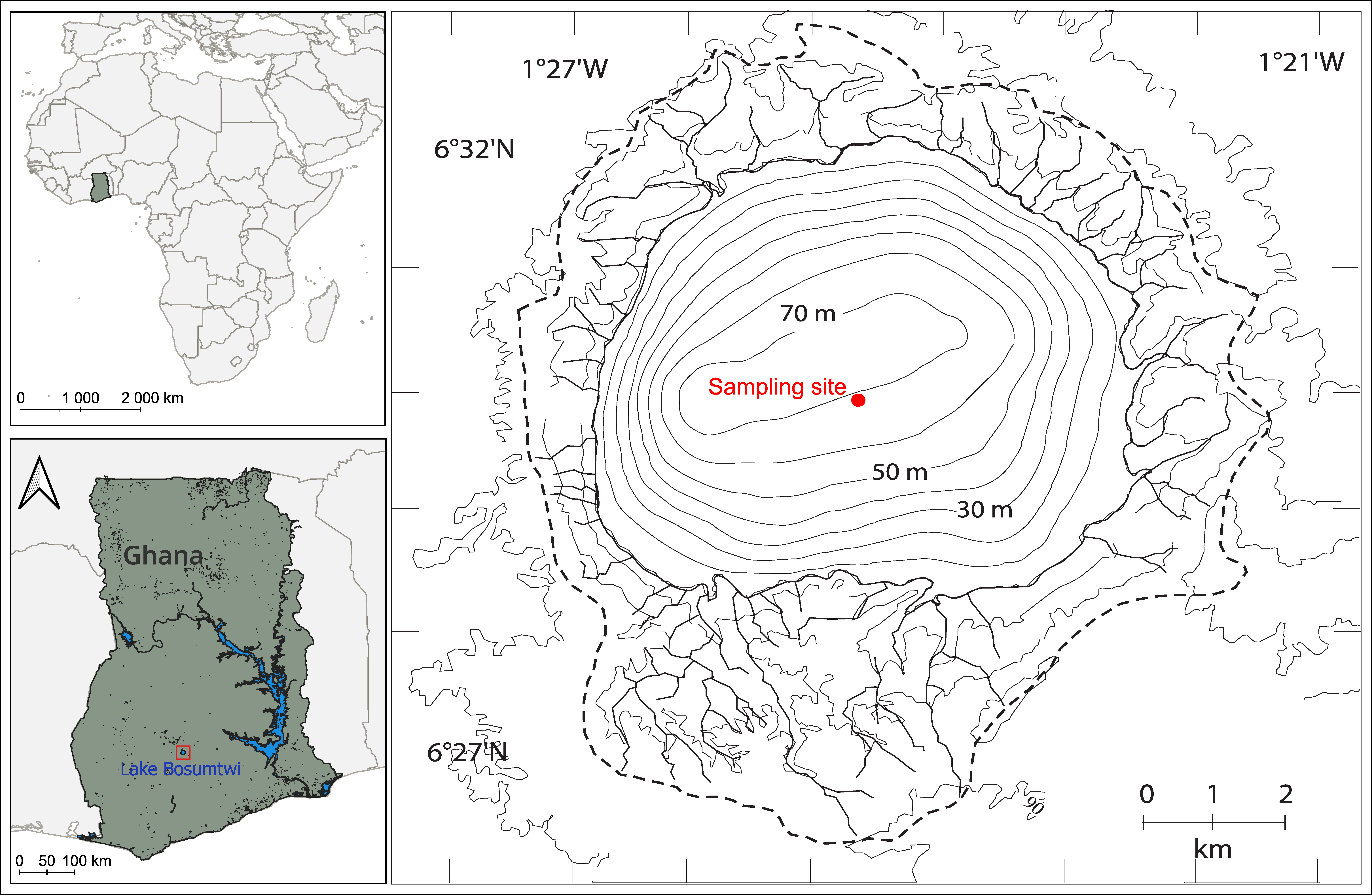
Lake Bosumtwi (Figure 1) is a deep, tropical, closed crater lake formed by a meteorite impact 1.07 million years ago [45,46,47]. The lake is located at 6°30′ N, 1°25′ W, at an elevation of 99 m a.s.l. in the south-central region of Ghana, West Africa. The crater is characterised by high walls rising to 460 m above the lake surface. However, groundwater input is highly restricted due to a thick layer of sediment [46]. The crater has a diameter of 10.5 (±0.5) km, whereas the lake surface has a diameter of 8–8.5 km. The lake has a maximum depth of 81 m, an average depth of 45 m, and a surface area of 52 km2 [45,47,48]. The hydrology of the lake is principally determined by relative annual rates of precipitation and evaporation, with 80% of the water balance dictated by direct rainfall on the lake surface. Rainfall is seasonally high, with a primary peak in May/June and a secondary peak in September/October. The pronounced crater walls restrict wind-generated mixing of the water column [49]. The lake is strongly stratified with a well-mixed epilimnion and an anoxic hypolimnion below a depth of 15–18 m [49,50,51]. Due to high wind speeds, low maximum daily atmospheric temperature, high daily average humidity [50], and the combined effects of high evaporation and radiative cooling of surface waters [52], deep annual mixing frequently occurs in August, resulting in a complete overturn [49,50,52].
Seasonal variability in the water column is driven by stratification and mixing patterns that exhibit high interannual variability concerning the timing, duration, and intensity of mixing events [50]. The lake is characterised by distinct stratification and mixing cycles, which show strong interannual variability, with wide fluctuations in mixing depth [50,51]. The thermocline, usually found at a depth of 8–10 m during the long-stratified period, fluctuates seasonally to depths of 30–40 m and below, depending on the intensity of convective cooling and wind stress [50]. Unlike in the past, the lake is no longer turning over completely, which may be indicative of climate warming effects. As such, the lake has shifted from holomixis to meromixis, marked by permanent anoxia below 30 m and the exclusion of seasonal circulation from the deepest part of the lake [49,50].
Dissolved inorganic nitrogen (DIN), total phosphorus (TP), soluble reactive phosphorus (SRP), pH, temperature, dissolved oxygen, conductivity, and chlorophyll a all show strong vertical gradients in the water column [29,50]. There is high nutrient enrichment in the deep, anoxic waters [49,50,55], due to prolonged stratification and less intense mixing. In addition, gases such as CO2 (average concentration of 59 µmol L−1), H2S, NH4 and CH4 have been found in deep water [50,55]. The usually hypoxic mid-water (depth of 12.5–30 m) hosts a deep chlorophyll maximum (DCM) that peaks (>100 µg L−1 chlorophyll a) during the stratified period (usually in May/June), coinciding with increased lake transparency [51,56]. The water chemistry is characterised by an average pH of 8.9 (above 9 in surface water above the thermocline), average conductivity of 1150 µS cm−1, and an acid-neutralising capacity of 10.32 mEq L−1 [50]. The lake supports a phytoplankton community historically dominated in biomass by cyanobacteria but also containing chlorophytes, dinoflagellates, diatoms, cryptophytes, and other algal groups; a fish community dominated by cichlids; and a species-poor pelagic zooplankton community [57,58,59]. Historical surveys identified nine zooplankton taxa, including a single crustacean copepod, the endemic cyclopoid M. bosumtwii, a single cladoceran, Moina micrura Kurz, 1875, six rotifer taxa, and larvae of the phantom midge Chaoborus ceratopogones (Theobald, 1903) [51,60,61].

2.2. Acquisition and Harmonisation of Historical Data

Historical data used for period 1 were obtained from surveys conducted at the central deep-water station of Lake Bosumtwi between January 2005 and December 2006 [50,51,61,62]. These data included water temperature, dissolved oxygen, nutrient concentrations, lake transparency measured by Secchi depth, and zooplankton body size, density, and biomass. In the historical study, zooplankton were sampled biweekly using a 70 µm mesh plankton net with a 25 cm mouth diameter and vertical hauls through the oxic habitat layer. The historical dataset was based on original field and laboratory measurements and was harmonised with the recent dataset using the same taxonomic groups, units, and biomass-calculation framework. Biweekly historical observations were aggregated into monthly values before comparison with the monthly observations from 2018 to 2020. The methods used to generate the recent dataset are described separately in Section 2.3, Section 2.4, Section 2.5, Section 2.6, Section 2.7 and Section 2.8.

2.3. Water Column Profiles and Determination of Thermal Structure

Depth profiles of water temperature, dissolved oxygen, pH, and conductivity were measured monthly using a YSI EXO2 multiparameter sonde (YSI Incorporated, Yellow Springs, OH, USA) from the surface to a depth of 70 m, at a downward rate of 10 cm s−1, from June 2018 to October 2020. Vertical water-column profiles were measured at a central deep-water station (6°30′06.4″ N, 1°24′42.6″ W). Transparency was measured with a Secchi disc (KC Denmark A/S, Silkeborg, Denmark). Measurements of dissolved oxygen (with an accuracy of ±0.1 mg L−1) were obtained in conjunction with temperature data (with an accuracy of ±0.01 °C). The instrument automatically adjusted conductivity measurements to a standard reference temperature of 25 °C. The equivalent historical data for 2005–2006 were collected using a Hydrolab H2O Multiprobe 6SBP (Hydrolab Corporation, Austin, TX, USA) from the surface to a depth of 50 m at the same sampling site. Data from both the YSI EXO2 and the Hydrolab underwent quality checks, and any anomalies presumed to stem from transcription errors or sensor malfunctions were excluded. Direct cross-calibration between the Hydrolab and the YSI EXO2 was not possible because the historical instrument was no longer available; however, both instruments were calibrated according to the manufacturers’ procedures, and the YSI EXO2 was verified using certified standards before field deployment. Dissolved oxygen readings of ≤0.20 mg L−1 were recorded as 0.00 mg L−1, indicating anoxic conditions. The thermal structure of the lake was determined using the algorithm developed by Xu et al. [63]. This approach allowed for the identification of the depths of the thermocline, as well as the precise locations of the lower epilimnion and upper hypolimnion.

2.4. Sample Collection

Water samples for the analysis of total nitrogen (TN) and total phosphorus (TP) were collected at 15 discrete depths from the surface to a depth of 65 m using a 6 L Niskin sampler (KC Denmark A/S, Silkeborg, Denmark). Samples from the surface to 20 m were collected at 2 m intervals, followed by 10 m intervals from 20 to 40 m and then at 55 m and 65 m. Similarly, for chlorophyll a analysis, samples were collected at 10 discrete depths within the upper 15 m. Samples for TN and TP were stored cold and in the dark until chemical analysis. Samples for chlorophyll a were immediately placed on ice, transported to the laboratory, filtered within 24 h of collection, and the filters were frozen until ethanol extraction and spectrophotometric analysis within 48 h. The same ethanol-extraction procedure was used for the historical and recent datasets.

2.5. Laboratory Analyses

To determine total phosphorus (TP), the acid persulfate digestion followed by the molybdate–ascorbic acid colorimetric method was used. Approximately 10 mL of the filtered water sample was transferred to a reagent flask. Then, 100 µL of 4 M sulfuric acid solution was added, and the sample was autoclaved at 121 °C for 30 min. After cooling, 400 µL of 50 g L−1 ascorbic acid solution and 400 µL of molybdate–antimony reagent were added. Absorbance was measured at 880 nm using a Shimadzu UV-1800 spectrophotometer (Shimadzu Corporation, Kyoto, Japan). The TP concentration was subsequently calculated using the TP calibration curve. Total nitrogen (TN) was measured using the alkaline persulfate digestion followed by the Griess–vanadium colorimetric determination of nitrate. First, 5 mL of each unfiltered water sample was transferred to a reagent flask. Then, 5 mL of Ox TN solution was added, and the mixture was autoclaved at 121 °C for 30 min. After cooling, 0.25 mL of Griess reagent and 0.525 mL of vanadium chloride reagent were added. The mixture was mixed and incubated in a 60 °C water bath for 30 min. The mixture was then cooled in a 25 °C water bath. Absorbance was measured at 540 nm, and the TN concentration was determined with the Shimadzu UV-1800 spectrophotometer using the TN calibration curve. Chlorophyll a concentration was determined using the ethanol extraction method and the Shimadzu UV-1800 spectrophotometer. Absorbance was measured using an installed photometric 8λ programme at λ1 = 665 nm and λ2 = 750 nm. Before each analytical session, the spectrophotometer was calibrated using certified reference standards and reagent blanks, and wavelength accuracy and absorbance stability were verified at the beginning of each analytical batch.

2.6. Zooplankton Sampling

Monthly sampling was conducted at a fixed central location from June 2018 to October 2020 (period 2), between 9:00 a.m. and 12:00 p.m., using a plankton net with a 70 μm mesh and a 25 cm mouth diameter. On each day before zooplankton sampling, the temperature and oxygen depth profiles from the YSI EXO2 were analysed on board to establish the thermocline and the depth of the oxic/zooplankton habitat layer within which zooplankton were distributed for the subsequent collection of zooplankton samples. Vertical hauls through the oxic layer were subsequently carried out in three replicates. Sampled zooplankton were preserved in 4% formalin and stored in the laboratory for subsequent processing and enumeration. The use of vertical tows through the oxic habitat layer at a fixed central station was consistent with the protocol used in the 2005–2006 study. Previous research indicates that Lake Bosumtwi exhibits limited horizontal heterogeneity in zooplankton distribution and that vertical gradients dominate community structure [62]. The 29-month time series provides a consistent representation of temporal pelagic zooplankton dynamics at the central deep-water station but does not quantify whole-lake horizontal variability.

2.7. Taxonomic Identification and Enumeration of Zooplankton

Taxonomic identification was conducted using the taxonomic keys for tropical freshwater zooplankton [64]. Confirmatory identifications were performed in the zoology laboratory of the Department of Ecology at the University of Presov, Slovakia. In the laboratory, zooplankton samples were filtered and washed with distilled water to remove the formalin preservative. The residual sample was then made up to a volume of 200 mL with distilled water. A subsample of 1 mL was taken from the well-mixed sample using a pipette and transferred to a Sedgwick-Rafter counting chamber (Graticules Optics, Tonbridge, Kent, UK). Samples were counted under a compound light microscope at 400× magnification. Three 1 mL subsamples were counted, and the coefficient of variation among replicate counts was usually below 10%. Abundance was calculated by extrapolating the mean subsample count to the total concentrated sample and dividing the estimated number of individuals by the volume of water filtered during the vertical haul. Abundance estimates from the three replicate vertical hauls were averaged and expressed as individuals m−3. Historical pelagic surveys recorded six rotifer taxa, of which Brachionus calyciflorus Pallas, 1766 and Hexarthra intermedia (Wiszniewski, 1929) were the dominant and most consistently recorded species, whereas the other four pelagic taxa occurred irregularly and generally at lower abundances [51,61,62]. A later, broader survey including both pelagic and littoral habitats increased the known rotifer richness of Lake Bosumtwi to 21 taxa [65]. No other copepod species are known from Lake Bosumtwi. Adult copepods were identified as the endemic cyclopoid M. bosumtwii, whereas naupliar and copepodite stages were assigned to this species based on the absence of any other known copepod species in the lake [60,61,62,66].

2.8. Biomass Determination, Body Length and Dry Weight Measurements

The total body length of 50 individuals per major taxon or developmental stage was measured using a calibrated horizontal ocular micrometre (Graticules Optics, Tonbridge, Kent, UK) attached to the eyepiece of a compound light microscope (Carl Zeiss AG, Oberkochen, Germany). For crustaceans, individual dry weight (W) was estimated using the taxon- or stage-specific operational length–weight relationships listed in Table 1. To maintain consistency with the historical Bosumtwi dataset, the equations reported in Table 1 were treated as the operational equations for biomass calculation in the present comparative analysis. These equations were based on published relationships, historical Bosumtwi calculations, and taxon-specific assumptions applied in the 2005–2006 study. For crustacean taxa, the original Bosumtwi workflow was based on allometric length–weight modelling of the form W = aLb, combining Bosumtwi-derived size–weight information with published regressions and parameter adjustments where required. In particular, the naupliar length–weight equation in the historical and current Bosumtwi studies was extracted from Culver et al. [67] with an adjustment of slope. Rotifer dry weight and biomass were calculated only for B. calyciflorus and H. intermedia, because these species represented the dominant and most consistently recorded rotifers in the pelagic samples, whereas the remaining rotifer taxa occurred irregularly and at low abundance [51,61,62]. For rotifers, dry weight estimation followed biovolume-based relationships derived from Ruttner-Kolisko [68], subsequently converted to dry weight under the assumptions applied in the historical Bosumtwi analysis. Fresh weights were computed assuming a specific gravity of 1 and were subsequently converted to dry weight by assuming that dry weight represented 10% of fresh weight [69]. The final equation for H. intermedia was V = 0.26 ab2, where V is biovolume, a is body length, and b is body width. The ratio of b to a was calculated as 0.694, expressed as b = 0.694 a. This relationship was then substituted for b in the first equation. Thus, the final biovolume relation was V = 0.125 a3. Similarly, the final biovolume equation for B. calyciflorus was V = 0.276 a3. For H. intermedia, 33% of the initial biovolume was taken as the biovolume of the appendages [68], which was added to the initial biovolume to obtain a final biovolume of the organism. The equations listed in Table 1 were applied consistently to both periods to standardise cross-period biomass comparisons. Mean individual dry weight (Dwt) for each taxon or developmental stage was calculated as the average of individual W values. Biomass was then estimated as B = (Dwt × A)/1000, where B is taxon-specific biomass (mg dwt m−3), Dwt is mean individual dry weight (µg dwt ind.−1), and A is abundance (ind. m−3). Descriptive values were calculated from months with recorded occurrence only, whereas graphical monthly distributions include zero values where applicable. Accordingly, taxon-specific dry weights should be interpreted as equation-derived estimates rather than universally transferable species-specific constants; however, the consistent use of the same equations across both periods allows robust comparison of period-level biomass patterns. In summary, body lengths were measured directly under a calibrated microscope and were not derived from the operational length–weight equations. The equations were used solely to convert empirically measured lengths into dry weight estimates for biomass calculations.

2.9. Statistical Analyses

Data were organised into monthly values for statistical comparisons and annual values for descriptive summaries and visualisation. Monthly means, rather than individual replicate hauls or individual depth measurements, were treated as the temporal sampling units in comparisons of zooplankton biomass and the ZB/Chl-a ratio. To standardise comparisons between the two study periods, the water column was divided into fixed depth strata corresponding approximately to the epilimnion (0–15 m), metalimnion (15–25 m), and hypolimnion (>25 m). The 15 m boundary was selected to approximate the mean thermocline depth across the study periods, although the actual thermocline depth varied among sampling dates. For the statistical analyses, significant differences were established at a 95% confidence level (p < 0.05). An independent-samples t-test was conducted to assess differences in water temperature and oxygen concentrations between the two periods, after validating the assumptions of normality and homogeneity of variance using the Shapiro–Wilk test and Levene’s test, respectively. The monthly zooplankton biomass-to-chlorophyll a ratio (ZB/Chl-a) was calculated as an index of relative zooplankton standing biomass per unit chlorophyll a. Differences in this ratio between the two periods (2005–2006 vs. 2018–2020) were evaluated using a Mann–Whitney U test based on monthly values. Because monthly observations may exhibit seasonality and temporal autocorrelation, the resulting significance levels were interpreted together with effect sizes and the consistency of patterns across environmental variables.
A one-way ANOVA was used to test for significant differences in zooplankton biomass across the years 2005, 2006, 2018, 2019, and 2020, with year as the grouping factor (independent variable) and biomass as the dependent variable. The data were first tested for normality and homogeneity of variance using the Shapiro–Wilk test and the median-centred Levene test, respectively. Where the test for homogeneity of variance was significant (p < 0.05), indicating violation of the equal-variance assumption, the Welch test was applied. A significant result (p < 0.05) was used to reject the null hypothesis of no difference in zooplankton biomass among years. Post hoc Games–Howell tests were used to determine which pairs of years differed significantly in biomass. Effect sizes were also computed to quantify the proportion of variance in biomass explained by differences among years. Statistical analyses were performed with IBM SPSS Statistics version 27.

3. Results

3.1. Patterns of Lake Temperature Change

The results show variable but significant warming across the water column between period 1 and period 2, with the strongest warming in the epilimnion (+0.30 °C), followed by the hypolimnion (+0.27 °C) and metalimnion (+0.27 °C) (Table 2; t-test: t(10, 980) = 16.3, p < 0.001). These patterns indicate consistent warming across all strata over the approximately 15-year interval separating the two study periods. Mean thermocline depth was 0.53 m shallower, decreasing from 11.07 ± 6.28 m in period 1 to 10.54 ± 0.68 m in period 2; however, this difference was small relative to the temporal variability in period 1.

3.2. Trends in Dissolved Oxygen, Nutrients, Chlorophyll a, and Water Transparency

Mean dissolved oxygen decreased significantly (t-test: t(22) = 3.208, p < 0.05) from 5.88 mg L−1 in period 1 to 4.32 mg L−1 in period 2, representing a decline of approximately 27%. Epilimnetic TP and TN concentrations were higher in period 2 than in period 1 (Table 3). Mean chlorophyll a concentration within the upper 15 m zone in period 1 was 8.07 µg L−1, rising to 19.49 µg L−1 in period 2 (Table 3). The 142% increase in chlorophyll a concentration between the two periods was significant (t-test: t(22) = −3.345, p < 0.01). According to the OECD trophic-state classification [70], mean chlorophyll a concentration in 2005–2006 was at the upper boundary of the mesotrophic range, whereas the substantially higher value in 2018–2020 was at the lower boundary of the eutrophic range. Consistent with this increase, mean Secchi depth decreased from 1.46 ± 0.28 m in period 1 to 1.18 ± 0.22 m in period 2, representing a 19% reduction in lake transparency. Habitat-layer depth, temperature, and dissolved oxygen, together with selected epilimnetic nutrient variables, chlorophyll a, and water transparency, are summarised in Table 3 to provide environmental context for the sampled habitat layer.

3.3. Trends and Variability in Zooplankton Body Size, Density, and Biomass

Table 4 provides a descriptive comparison of taxon- and stage-specific body size, equation-derived dry weight, density, and biomass between the two study periods; these differences should be interpreted as descriptive unless inferential statistics are explicitly reported. Mean naupliar length was 16% lower in period 2, decreasing from 0.20 ± 0.01 mm to 0.17 ± 0.03 mm. Estimated mean dry weight and mean biomass of nauplii both decreased between periods, with mean biomass declining from 44.4 ± 25.5 to 33.3 ± 19.5 mg dwt m−3. Maximum naupliar biomass decreased from 103.7 mg dwt m−3 in period 1 to 88.2 mg dwt m−3 in period 2. In contrast to nauplii, copepodite body size increased along with estimated mean dry weight. Copepodite mean length increased by 19%, from 0.52 ± 0.08 mm in 2005–2006 to 0.62 ± 0.07 mm in 2018–2020, while estimated mean dry weight increased by 20% from 22.0 ± 2.9 to 26.4 ± 3.1 µg dwt ind.−1. Copepodite densities increased markedly between periods, resulting in a strong increase in biomass in period 2.
Adult M. bosumtwii increased in mean body length, estimated individual dry weight, density, and biomass during period 2. Mean body length increased by 19%, while adult biomass increased by approximately 72%. Maximum body length was also higher in period 2, following a pattern broadly similar to that observed in copepodites (Table 4). The increase in adult biomass reflected the combined effects of greater body length, the associated increase in estimated individual dry weight, and higher density.

3.4. Observed Shifts in Cladoceran Body Size, Density, and Biomass

Cladocera, represented by a single species (M. micrura), showed declines in body size and biomass, with lower variability in density and biomass during period 2 (Table 4). Decreases were observed in mean length, estimated mean dry weight, abundance, and occurrence-based mean biomass. Mean biomass calculated from months with recorded occurrence decreased descriptively by approximately 30%, from 15.2 ± 26.5 mg dwt m−3 in period 1 to 10.7 ± 9.0 mg dwt m−3 in period 2. However, because cladoceran biomass did not differ significantly among years, these changes should be interpreted as descriptive trends.

3.5. Observed Shifts in Body Size, Density, and Biomass of Dominant Rotifers

The analysis of rotifer body-size and biomass metrics focused on the two dominant pelagic species, B. calyciflorus and H. intermedia [51,61,62]. Brachionus calyciflorus showed changes in body-size and biomass metrics between periods. The mean length increased from 0.21 ± 0.02 mm in period 1 to 0.22 ± 0.03 mm in period 2 (Table 4). The estimated mean dry weight increased slightly from 0.26 ± 0.06 µg in period 1 to 0.31 ± 0.06 µg in period 2. Downward trends in mean density and mean biomass were also observed. The reduction in mean biomass was driven by the pronounced decline in population density, despite the slight increase in estimated mean dry weight. In period 2, rotifer biomass remained low, with especially small values for B. calyciflorus and a low combined biomass contribution from the two rotifer taxa. For H. intermedia, mean length and estimated mean dry weight increased slightly, whereas density and biomass declined markedly between periods (Table 4). Mean length changed only slightly, from 0.12 ± 0.03 mm in period 1 to 0.12 ± 0.04 mm in period 2. However, because rotifer biomass was estimated from equation-based dry-weight conversions, the observed rotifer biomass pattern should be interpreted primarily as an outcome of the applied historical biomass-estimation framework rather than as direct evidence of proportional change in all morphological traits. Accordingly, the rotifer results are best treated as comparative descriptive estimates derived under a standardised operational procedure across periods. The small differences in mean individual size between periods should also be interpreted cautiously, because rotifers show limited post-embryonic somatic growth due to eutely; in addition, B. calyciflorus may exhibit polymorphism, which can contribute to body-size variation independently of simple growth responses.

3.6. Variability in Biomass Among Zooplankton Assemblages

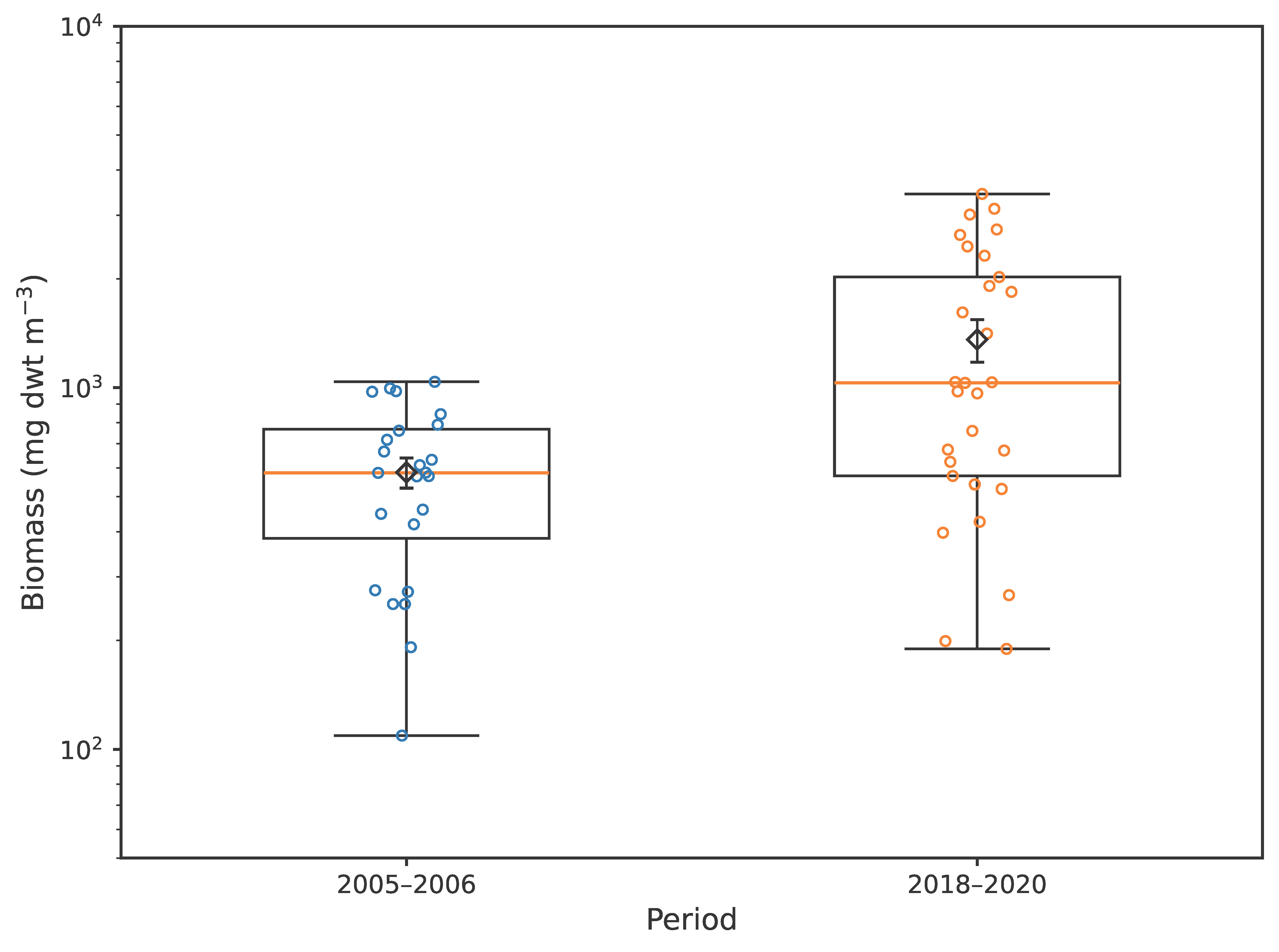
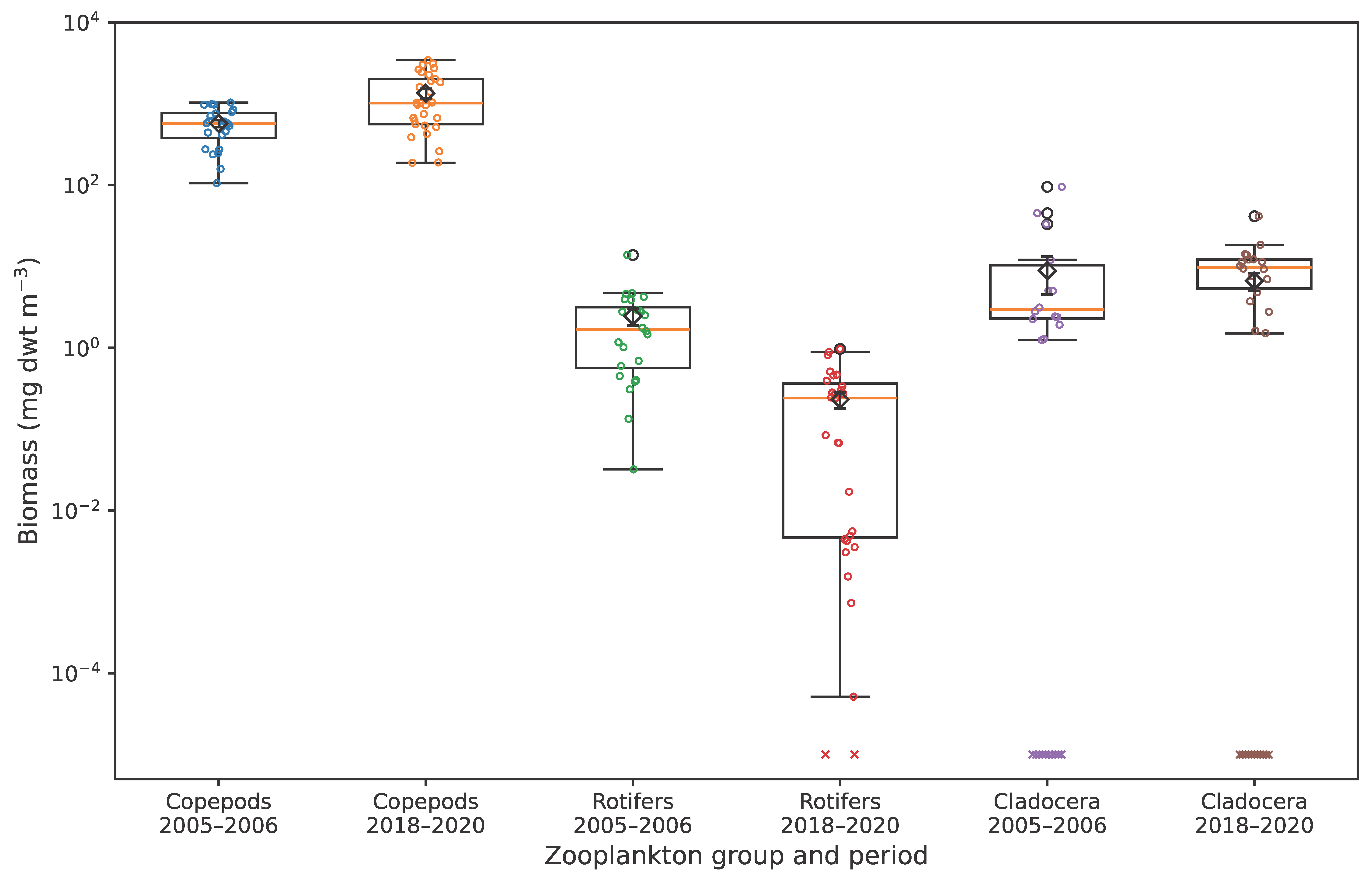
Copepods dominated zooplankton biomass in both study periods, indicating a persistent community biomass structure. However, total zooplankton biomass was markedly higher in 2018–2020 than in 2005–2006 (Figure 2). This period-level contrast is consistent with the year-level inferential analyses reported below, which detected significant differences among years in total zooplankton and copepod biomass. Group-specific comparisons show that the increase in total zooplankton biomass was driven primarily by higher copepod biomass, whereas rotifer biomass was lower in 2018–2020 and cladoceran biomass remained highly variable, with no significant difference among years (Figure 3). Overall, these patterns indicate a marked increase in total zooplankton biomass and substantially higher absolute copepod biomass in the recent period.

3.7. Temporal Variability in Biomass of Major Zooplankton Groups

Copepod biomass was substantially higher and more variable in 2018–2020 than in 2005–2006, with several pronounced peaks during the recent period. Rotifer biomass was markedly lower in 2018–2020 than in 2005–2006, although occasional short-lived peaks occurred in both periods. Cladoceran biomass (represented by the single species, M. micrura) was highly variable in both periods, with numerous zero-occurrence months and occasional biomass peaks; no significant difference among years was detected. Detailed monthly time-series plots for total zooplankton biomass and the three major groups are provided in Supplementary File S1 (Figures S1–S4); additional environmental summaries are provided in Figure S5 and Table S1.

3.8. Copepod Biomass Dynamics and Temporal Variability

Copepod biomass dynamics differed between the two periods in magnitude, timing of peaks, seasonality, and variability. During the first period, copepod biomass ranged from 105.3 to 1035.4 mg dwt m−3, whereas in the recent period it ranged from 187.6 to 3435.6 mg dwt m−3, indicating substantially higher biomass and greater variability in 2018–2020 (Supplementary File S1, Figure S2). The maximum monthly copepod biomass was approximately 3.3 times higher in the recent period. Distinct peaks were observed in July and September 2005, whereas the highest biomass values in 2006 occurred in October and December. Biomass increases occurred during both mid-year and late-year months, with pronounced monthly variability in both periods. In the recent period, the highest copepod biomass occurred in October 2019, and the amplitude of monthly fluctuations was substantially greater than in 2005–2006.

3.9. Rotifer Biomass Dynamics and Temporal Variability

Rotifer biomass ranged from 0.03 to 13.8 mg dwt m−3 during the first period, with the maximum recorded in August 2005. During the second period, rotifer biomass was substantially lower, ranging from 0 to 0.97 mg dwt m−3, with the maximum recorded in August 2019 (Supplementary File S1, Figure S3). The recorded peaks in August in both periods indicate a strong seasonal signal in rotifer biomass dynamics. During period 1, the highest rotifer biomass values occurred between July and August. Rotifer biomass fluctuated markedly during period 1. In contrast, the amplitude of biomass fluctuations during the second period was markedly lower.

3.10. Cladoceran Biomass Dynamics and Temporal Variability

Cladoceran biomass was highly episodic in both periods, with numerous zero-occurrence months and occasional short-lived peaks. In 2005–2006, biomass ranged from 0 to 94.9 mg dwt m−3, with the maximum recorded in September 2006. In 2018–2020, biomass ranged from 0 to 41.4 mg dwt m−3, with the maximum recorded in November 2019 (Supplementary File S1, Figure S4).

3.11. Zooplankton Biomass-to-Chlorophyll a Ratio (ZB/Chl-a)

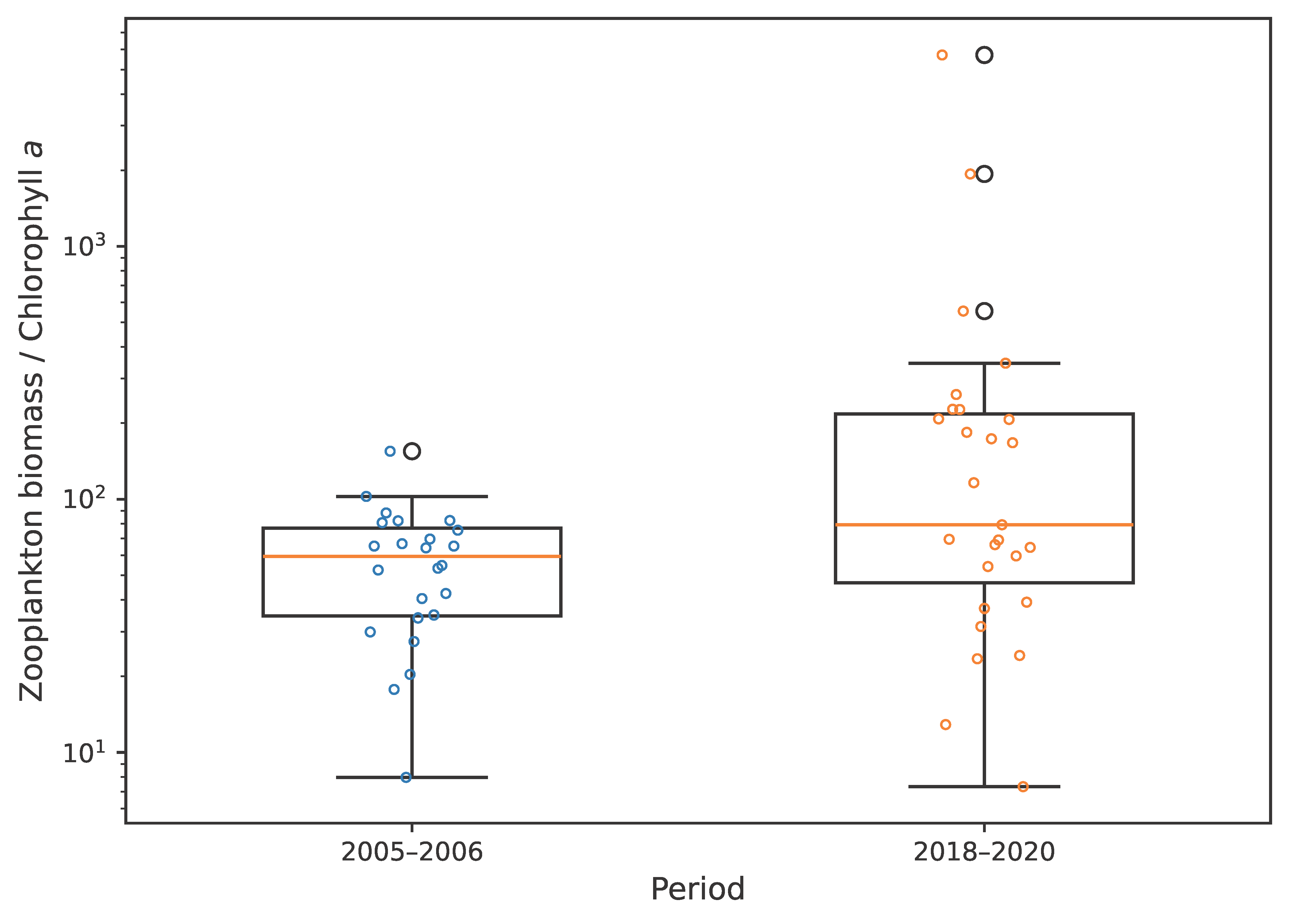
Mean monthly total zooplankton biomass increased approximately 2.33-fold, from 582.8 ± 272.2 mg dwt m−3 in period 1 to 1359.5 ± 983.2 mg dwt m−3 in period 2. Maximum monthly community biomass increased from 1037.9 mg dwt m−3 in period 1 to 3435.9 mg dwt m−3 in period 2. The zooplankton biomass-to-chlorophyll a ratio (ZB/Chl-a) differed significantly between the two periods (Figure 4), indicating higher zooplankton biomass relative to chlorophyll a concentration in 2018–2020. Median ZB/Chl-a increased from 59.46 (IQR 34.67–76.75) in 2005–2006 to 79.24 (IQR 46.66–217.08) in 2018–2020 (Mann–Whitney U = 210, p = 0.032).

3.12. Summary of Statistical Analyses

The inferential results below support the period- and year-level biomass contrasts visualised in Figure 2 and Figure 3. Welch’s ANOVA detected significant differences among years in copepod biomass (F = 4.66, p = 0.007), rotifer biomass (F = 13.77, p < 0.001), and total zooplankton biomass (F = 4.62, p = 0.008), whereas a conventional one-way ANOVA detected no significant difference among years in cladoceran biomass (F(4, 48) = 0.718, p = 0.584). Because variances were unequal for copepod, rotifer, and total zooplankton biomass, Welch’s ANOVA was applied to these groups, whereas conventional one-way ANOVA was used for cladocerans. For total zooplankton biomass, year explained approximately 36% of the observed variance (η2 = 0.358; ε2 = 0.305). These effect sizes indicate a substantial year-related component in total zooplankton biomass across the five sampled years, grouped into two study periods separated by approximately 15 years. Games–Howell post hoc tests showed significant differences in copepod and total zooplankton biomass between 2005 and 2019, between 2006 and 2019, and between 2018 and 2019; the remaining pairwise comparisons were not significant. Biomass did not differ significantly between 2005 and 2006 or between 2019 and 2020, whereas 2018 and 2019 differed significantly for copepods and total zooplankton. Rotifer biomass differed significantly among years (Welch’s ANOVA, p < 0.001), whereas cladoceran biomass did not (one-way ANOVA, F(4, 48) = 0.718, p = 0.584). For rotifers, significant Games–Howell differences occurred between 2006 and each of 2018, 2019, and 2020; between 2018 and 2020; and between 2019 and 2020. The effect of year was moderate for rotifer biomass (η2 = 0.300; ε2 = 0.242) and small for cladoceran biomass (η2 = 0.045).

4. Discussion

4.1. Effects of Lake Warming on Thermal Structure and Lake Habitat Quality

Between 2005–2006 and 2018–2020, temperatures increased across all thermal layers, most strongly in the epilimnion, while the mean temperature of the oxic/zooplankton habitat layer remained broadly similar. This pattern is consistent with current understanding of lake thermal dynamics under atmospheric warming trends [11,29]. The epilimnion is especially susceptible to heating because it receives most of the solar radiation and is directly exposed to atmospheric heat exchange. These processes are further intensified under currently elevated air temperatures, contributing to the greater warming observed in the epilimnion [71]. In contrast, the hypolimnion remained relatively insulated from atmospheric heating and warmed less.
Warming across all strata, with the strongest increase in the epilimnion, was accompanied by a shallower thermocline in the recent period. This phenomenon reduced mixing depth, increased water column stability, and increased resistance to seasonal mixing [12,72]. Hypolimnetic oxygen depletion limits habitable space for zooplankton populations, resulting in decreased abundance [73]. The ecological consequences of warming include alterations in community structure, disruption of diel vertical migration, growth and reproductive stress, and feedback to nutrient cycling. In this feedback, changing nutrient dynamics modify phytoplankton composition, which in turn affects food availability for zooplankton [74,75].
Another indicator of changing habitat conditions is the approximately 27% decrease in dissolved oxygen in the oxic/zooplankton habitat layer, from 5.88 mg L−1 in period 1 to 4.32 mg L−1 in period 2. The shallower mean thermocline and lower dissolved oxygen may have compressed zooplankton into upper waters, disrupting vertical migration and increasing predator–prey overlap [74,76]. Hypolimnetic oxygen depletion and shrinking habitat space can also alter competition among zooplankton [11]. Habitat compression increases interspecific competition for limited food resources, mainly phytoplankton [77]. Additionally, resource partitioning breaks down because shrinking habitat spaces collapse niches established by vertical stratification, thereby intensifying niche overlap [78,79].

4.2. Changes in Dissolved Oxygen and Implications for Zooplankton

The reduction in mean dissolved oxygen from 5.88 mg L−1 in period 1 to 4.32 mg L−1 in period 2 raises the question of whether such levels imposed taxon-specific physiological constraints despite the observed increase in total zooplankton biomass. Zooplankton differ markedly in oxygen tolerance: rotifers often persist at very low dissolved oxygen (DO), including near-anoxic conditions, although their biomass declines sharply as DO falls below 1 mg L−1 [73]. Under such conditions, they can maintain biomass where crustaceans decline, promoting shifts toward smaller-bodied taxa and altered community structure [80]. Copepods and cladocerans are less tolerant, with biomass-decline thresholds of approximately 1.5–3 mg O2 L−1 and 2–4 mg O2 L−1, respectively [81,82,83]. Although DO decreased by approximately 27% between the two periods, concentrations in the sampled oxygenated habitat remained within reported tolerance ranges and did not prevent the substantial increase in copepod-dominated biomass. Oxygen decline alone cannot explain the observed responses, which likely reflect its interaction with habitat compression, food availability, predation, competition, and taxon-specific feeding strategies.

4.3. Changes in Nutrient Dynamics and Phytoplankton Biomass

The upward migration of the thermocline, with corresponding expansion of the anoxic hypolimnion and reduced DO, has led to a significant change in nutrient fluxes within Lake Bosumtwi. One notable consequence is the exceptionally high nutrient buildup in deep-water layers, which occurs because of diminished mixing of the water column concurrent with nutrient depletion in surface waters due to biological uptake by phytoplankton. Consequently, stratification and reduced mixing can lead to nutrient enrichment in deep waters and modification of nutrient availability in surface layers. Nutrient availability in the surface waters of Lake Bosumtwi is primarily driven by internal loading, which is strongly linked to climate-driven lake hydrodynamics [50], suggesting little contribution from the watershed. This situation remained relatively unchanged until recent years, when rapid deforestation and extensive crop farming began to alter the landscape. These changes in the landscape may have increased sediment and nutrient transport to the lake and contributed to greater external loading [84], although catchment nutrient inputs were not quantified directly in the present study.
Epilimnetic TP concentrations exceeded the cited threshold range in both periods, whereas TN was below the cited range in period 1 and within it in period 2. Therefore, the available total-nutrient data do not permit a definitive conclusion regarding nutrient limitation of phytoplankton productivity. Specifically, the cited threshold range is 0.01–0.02 mg P L−1 for TP and 0.30–0.50 mg N L−1 for TN [85,86]. Measured TP exceeded this range in both periods, whereas TN was below the cited range in period 1 and within it in period 2, suggesting that phosphorus limitation was unlikely but that potential nitrogen limitation in period 1 cannot be excluded. These results indicate that phosphorus was unlikely to limit phytoplankton growth in either period, whereas nitrogen limitation may have been more plausible in period 1 than in period 2. Consequently, external loading mechanisms may now exert a stronger influence on lake productivity, complementing or potentially surpassing the role of internal nutrient cycling. These shifts in nutrient dynamics have important implications for the lake’s ecological balance and for the processes regulating phytoplankton biomass and, by extension, zooplankton biomass.
Phytoplankton standing biomass, approximated by chlorophyll a, increased by 142% between the two study periods, in parallel with higher epilimnetic TP and TN concentrations. Historical studies indicate that phytoplankton biomass and productivity in Lake Bosumtwi also depend on mixing depth, light availability, and seasonal stratification, with TP alone showing weak predictive power [57,59,87]. A larger phytoplankton standing stock may also have supported protozoa and ciliates, which commonly increase with trophic status and chlorophyll a [88]. However, chlorophyll a is a proxy for standing biomass rather than production rate or food quality. Historical measurements showed high gross productivity but also high community respiration and comparatively low net growth [87]. The concurrent increases in nutrients and chlorophyll a may therefore have expanded both direct phytoplankton food and indirect protozoan, ciliate, and zooplankton prey resources available to the omnivorous M. bosumtwii. This pattern was accompanied by a significantly higher ZB/Chl-a ratio in 2018–2020 than in 2005–2006, indicating greater zooplankton standing biomass relative to chlorophyll a in the recent period (Figure 4). Previous studies of Lake Bosumtwi reported cyanobacterial dominance and a potential trophic bottleneck between primary producers and zooplankton [60,61]. However, phytoplankton taxonomic and size composition was not determined during 2018–2020, and the observed increase in chlorophyll a cannot therefore be attributed specifically to cyanobacteria. Previous studies of Lake Bosumtwi showed that cyanobacteria dominated phytoplankton biomass, while chlorophytes, dinoflagellates, diatoms, cryptophytes, and other groups were also present [57,58,59]. The increased standing stock in 2018–2020 may therefore have included both poorly edible cyanobacteria and more readily consumable algal resources. Consequently, the 2018–2020 food environment should be interpreted as quantitatively richer but taxonomically unresolved. A lake-wide survey conducted in 2015 found that cyanobacteria comprised more than 90% of phytoplankton abundance in both rainy and dry seasons, together with smaller contributions from green algae and diatoms [58], suggesting that cyanobacterial dominance may have persisted close to the recent study period. However, because phytoplankton composition was not measured concurrently in 2018–2020, its persistence during the present sampling period cannot be confirmed. Accordingly, the proposed mechanisms remain plausible but untested; the higher ZB/Chl-a ratio supports consideration of direct and indirect food-web pathways rather than a simple strengthening of the trophic bottleneck.
Despite lower dissolved oxygen, mean community zooplankton biomass increased approximately 2.33-fold between the two study periods. This increase was driven almost entirely by copepods, which accounted for approximately 98% of total zooplankton biomass in 2005–2006 and more than 99% in 2018–2020. The strongest increases occurred in copepodites and adults, whereas naupliar biomass declined, indicating a stage-specific response. Because later Mesocyclops stages increasingly exploit ciliates, rotifers, and small crustaceans in addition to suitable algae, greater availability of phytoplankton and associated animal prey may have particularly favoured copepodites and adults [24,25]. Rotifer biomass was substantially lower in 2018–2020, whereas M. micrura showed decreases in mean body length, density, and occurrence-based biomass. Experimental studies demonstrate that Mesocyclops can prey on B. calyciflorus and small cladocerans and that abundant Mesocyclops populations can substantially restructure communities of small zooplankton [24,26,44]. The increased biomass of copepodites and adults may therefore have intensified top-down predation pressure on rotifers and M. micrura. However, because predation was not measured directly and cladoceran biomass did not differ significantly among years, this pathway should be regarded as a plausible hypothesis, and the M. micrura response should remain classified as descriptive.
The higher ZB/Chl-a ratio indicates greater zooplankton standing biomass per unit chlorophyll a, but not necessarily greater trophic-transfer efficiency. Taken together, the observed community reorganisation is consistent with the combined effect of bottom-up and top-down processes. Higher epilimnetic TP and TN coincided with a 142% increase in chlorophyll a, indicating a larger but taxonomically unresolved phytoplankton standing stock. Greater algal availability may also have supported protozoan and ciliate prey, thereby expanding both direct and indirect food resources for M. bosumtwii [24,25,88]. The resulting increase in copepodites and adults may subsequently have strengthened predation pressure on rotifers and small cladocerans [26,44]. This proposed nutrient- and mixing-mediated phytoplankton–microbial prey–copepod–small zooplankton pathway provides a coherent explanation for the simultaneous increase in copepod biomass and reduction in smaller zooplankton. It is consistent with previous Lake Bosumtwi studies showing strong seasonal regulation of phytoplankton biomass and productivity by light-use efficiency, mixing, and stratification, together with persistent cyanobacterial dominance and the continued occurrence of other algal groups [57,58,59,87]. However, the individual trophic links were not tested directly.
A limitation of the study is that water-column profiles in the two periods were obtained using different multiparameter sondes, and direct cross-calibration was not possible because the historical instrument was no longer available. Although both instruments underwent quality control and the observed warming was consistent across all thermal strata, the relatively small inter-period temperature differences should be interpreted with this instrumentation constraint in mind, though indicators such as shallow thermocline and reduced DO strongly support evidence of warming. Individual dry weights and taxon-specific biomass values were derived from length–weight and biovolume relationships and may therefore be affected by systematic uncertainty associated with the selected equations. Nevertheless, the same equations were applied consistently to both study periods, supporting internal comparability of period-level biomass patterns. Directly measured body lengths are independent of these regressions, whereas absolute dry-weight estimates should not be interpreted as universally transferable species-specific constants. Another methodological limitation of this study concerns the treatment of temporal structure in the monthly time-series data. Because the observations exhibit clear seasonal patterns and likely temporal autocorrelation, the assumption of independence underlying the parametric tests may not be fully met. This implies that the effective sample size may be smaller than the nominal number of monthly observations, and the strength of statistical evidence should therefore be interpreted with appropriate caution. Interpretation is further limited by the use of a single central station and the absence of concurrent data on phytoplankton composition, primary production, microbial prey, diet, predation, fish, and catchment loading. Despite these limitations, coherent effect sizes and cross-variable patterns support the ecological relevance of the observed period-level differences.

5. Conclusions

Compared with 2005–2006, the 2018–2020 period was characterised by warmer and less oxygenated conditions and by higher epilimnetic TP, TN, and chlorophyll a concentrations. These differences coincided with a 2.33-fold increase in mean total zooplankton biomass, driven almost entirely by higher copepod biomass. The concurrent increases in nutrients, chlorophyll a, and copepod biomass are consistent with a bottom-up response in which a larger phytoplankton standing stock may have supported the copepod population. Historical studies indicate that the phytoplankton of Lake Bosumtwi includes both cyanobacteria and potentially more consumable algal groups, although cyanobacteria have generally dominated biomass [57,58,59]. Because chlorophyll a does not distinguish taxonomic composition, food quality, or net primary production, the precise basal resource responsible for the copepod response remains unresolved. The marked increase in copepodites and adults may, in turn, have strengthened top–down predation pressure on smaller zooplankton, providing a plausible explanation for the substantially lower rotifer biomass and the decline in M. micrura [26,44]. The contrasting responses among developmental stages and taxa indicate a shift toward a more strongly copepod-dominated pelagic food web rather than a uniform response of zooplankton to warming. Because phytoplankton composition, protozoan and ciliate prey, copepod diet, and direct predation rates were not measured, the proposed nutrient–phytoplankton–microbial prey–copepod–small zooplankton pathway should be regarded as a testable mechanistic hypothesis rather than as a demonstrated causal mechanism.

Supplementary Materials

The following supporting information can be downloaded at: https://www.mdpi.com/article/10.3390/limnolrev26030047/s1, Figure S1: Monthly dynamics of total zooplankton biomass (mg dwt m−3) in 2005–2006 and 2018–2020. Biomass is shown on a logarithmic scale; Figure S2: Monthly dynamics of copepod biomass (mg dwt m−3) in 2005–2006 and 2018–2020. Biomass is shown on a logarithmic scale; Figure S3: Monthly dynamics of rotifer biomass (mg dwt m−3) in 2005–2006 and 2018–2020. Biomass is shown on a logarithmic scale; zero values, where present, are displayed at the lower plotting limit; Figure S4: Monthly dynamics of cladoceran biomass (mg dwt m−3) in 2005–2006 and 2018–2020. Biomass is shown on a logarithmic scale; zero values, where present, are displayed at the lower plotting limit; Figure S5: Distributions of selected environmental variables in 2005–2006 and 2018–2020: temperature in the fixed 0–15 m epilimnetic layer, epilimnetic dissolved oxygen, epilimnion/oxic depth, total phosphorus, total nitrogen, and chlorophyll a. Boxplots show medians, interquartile ranges, 1.5 × IQR whiskers, and outliers; Table S1: Changes in selected nutrient variables, dissolved oxygen, chlorophyll a, and the zooplankton biomass-to-chlorophyll a ratio (ZB/Chl-a) in Lake Bosumtwi between period 1 (2005–2006) and period 2 (2018–2020). TP, total phosphorus; TN, total nitrogen; DO, dissolved oxygen; ZB/Chl-a, zooplankton biomass-to-chlorophyll a ratio; Table S2: Interannual and decadal changes in mean monthly zooplankton biomass (mg dwt m−3). Data for 2018 cover June–December and data for 2020 cover January–October. Period means were calculated from all available monthly observations. DIC, descriptive interannual change from 2005 to 2006 and from 2019 to 2020.

Author Contributions

Conceptualisation, P.S. and S.A.; methodology, P.S., S.A. and A.D.; software, P.S., R.S. and S.A.; validation, P.S. and R.S.; formal analysis, P.S., S.A. and R.S.; investigation, P.S., S.A. and A.D.; resources, P.S. and R.S.; data curation, P.S. and R.S.; writing—original draft preparation, P.S., R.S. and S.A.; writing—review and editing, P.S. and R.S.; visualisation, P.S. and R.S.; supervision, P.S. and R.S.; project administration, P.S.; funding acquisition, P.S. All authors have read and agreed to the published version of the manuscript.

Funding

This research was conducted as part of the Building Resilience of Lake Bosumtwi to Climate Change (RELAB) project, funded by the Ministry of Foreign Affairs of Denmark under grant No. 18-02-GHA. The grant was administered by the Danida Fellowship Centre. Field sampling was partially supported by the Erasmus+ Programme, project No. 2019-1-SK01-KA107-060299.

Data Availability Statement

The data presented in this study are openly available in Zenodo at https://doi.org/10.5281/zenodo.19567511. Source geospatial data used to create the location map of Lake Bosumtwi (Figure 1) were obtained from OpenStreetMap through the Geofabrik data-download service [89].

Acknowledgments

We thank the field and laboratory team of the RELAB project led by Eric Darko, Augustine Boakye, Krobea Asante and Boahen Gyau for assisting with fieldwork, laboratory analysis and associated logistics. Boat services to the central station of the lake were provided by John Bilson and George Ampong. During the preparation of this manuscript, the authors used the web-based versions of Microsoft Copilot (Microsoft Corporation, Redmond, WA, USA; accessed on 6 August 2026) and Grammarly (Grammarly, Inc., San Francisco, CA, USA; accessed on 6 August 2026) to review the manuscript and improve its grammar, language, structure, and readability. The authors have reviewed and edited the output and take full responsibility for the content of this publication.

Conflicts of Interest

The authors declare no conflicts of interest. The funders had no role in the design of the study, in the collection, analyses, or interpretation of data; in the writing of the manuscript, or in the decision to publish the results.

References

  1. Cremona, F.; Agasild, H.; Haberman, J.; Zingel, P.; Nõges, P.; Nõges, T.; Laas, A. How Warming and Other Stressors Affect Zooplankton Abundance, Biomass and Community Composition in Shallow Eutrophic Lakes. Clim. Change 2020, 159, 565–580. [Google Scholar] [CrossRef]
  2. Du, P.; Ye, W.-J.; Deng, B.-P.; Mao, M.; Zhu, Y.-L.; Cheng, F.-P.; Jiang, Z.-B.; Shou, L.; Chen, Q.-Z. Long-Term Changes in Zooplankton in the Changjiang Estuary from the 1960s to 2020. Front. Mar. Sci. 2022, 9, 961591. [Google Scholar] [CrossRef]
  3. Wang, C.; Li, E.; Zhang, L.; Wei, H.; Zhang, L.; Wang, Z. Long-Term Succession Characteristics and Driving Factors of Zooplankton Communities in a Typical Subtropical Shallow Lake, Central China. Environ. Sci. Pollut. Res. Int. 2023, 30, 49435–49449. [Google Scholar] [CrossRef] [PubMed]
  4. Zhang, C.; Brett, M.T.; Nielsen, J.M.; Arhonditsis, G.B.; Ballantyne, A.P.; Carter, J.L.; Kann, J.; Müller-Navarra, D.C.; Schindler, D.E.; Stockwell, J.D.; et al. Physiological and Nutritional Constraints on Zooplankton Productivity Due to Eutrophication and Climate Change Predicted Using a Resource-Based Modeling Approach. Can. J. Fish. Aquat. Sci. 2022, 79, 472–486. [Google Scholar] [CrossRef]
  5. Lee, H.; Calvin, K.; Dasgupta, D.; Krinner, G.; Mukherji, A.; Thorne, P.; Trisos, C.; Romero, J.; Aldunce, P.; Barrett, K.; et al. IPCC, 2023: Summary for Policymakers. In Climate Change 2023: Synthesis Report. Contribution of Working Groups I, II and III to the Sixth Assessment Report of the Intergovernmental Panel on Climate Change; Core Writing Team, Lee, H., Romero, J., Eds.; IPCC: Geneva, Switzerland, 2023; pp. 1–34. [Google Scholar]
  6. Cheung, W.W.L.; Lam, V.W.Y.; Sarmiento, J.L.; Kearney, K.; Watson, R.; Pauly, D. Projecting Global Marine Biodiversity Impacts under Climate Change Scenarios. Fish Fish. 2009, 10, 235–251. [Google Scholar] [CrossRef]
  7. Janse, J.H.; Kuiper, J.J.; Weijters, M.J.; Westerbeek, E.P.; Jeuken, M.H.J.L.; Bakkenes, M.; Alkemade, R.; Mooij, W.M.; Verhoeven, J.T.A. GLOBIO-Aquatic, a Global Model of Human Impact on the Biodiversity of Inland Aquatic Ecosystems. Environ. Sci. Policy 2015, 48, 99–114. [Google Scholar] [CrossRef]
  8. O’Reilly, C.M.; Sharma, S.; Gray, D.K.; Hampton, S.E.; Read, J.S.; Rowley, R.J.; Schneider, P.; Lenters, J.D.; McIntyre, P.B.; Kraemer, B.M.; et al. Rapid and Highly Variable Warming of Lake Surface Waters around the Globe. Geophys. Res. Lett. 2015, 42, 10773–10781. [Google Scholar] [CrossRef]
  9. Dahlke, F.T.; Wohlrab, S.; Butzin, M.; Pörtner, H.-O. Thermal Bottlenecks in the Life Cycle Define Climate Vulnerability of Fish. Science 2020, 369, 65–70. [Google Scholar] [CrossRef] [PubMed]
  10. Hébert, M.-P.; Beisner, B.E.; Rautio, M.; Fussmann, G.F. Warming Winters in Lakes: Later Ice Onset Promotes Consumer Overwintering and Shapes Springtime Planktonic Food Webs. Proc. Natl. Acad. Sci. USA 2021, 118, e2114840118. [Google Scholar] [CrossRef] [PubMed]
  11. Woolway, R.I.; Sharma, S.; Smol, J.P. Lakes in Hot Water: The Impacts of a Changing Climate on Aquatic Ecosystems. BioScience 2022, 72, 1050–1061. [Google Scholar] [CrossRef] [PubMed]
  12. Woolway, R.I.; Kraemer, B.M.; Lenters, J.D.; Merchant, C.J.; O’Reilly, C.M.; Sharma, S. Global Lake Responses to Climate Change. Nat. Rev. Earth Environ. 2020, 1, 388–403. [Google Scholar] [CrossRef]
  13. Grant, L.; Vanderkelen, I.; Gudmundsson, L.; Tan, Z.; Perroud, M.; Stepanenko, V.M.; Debolskiy, A.V.; Droppers, B.; Janssen, A.B.G.; Woolway, R.I.; et al. Attribution of Global Lake Systems Change to Anthropogenic Forcing. Nat. Geosci. 2021, 14, 849–854. [Google Scholar] [CrossRef]
  14. Gillooly, J.F.; Brown, J.H.; West, G.B.; Savage, V.M.; Charnov, E.L. Effects of Size and Temperature on Metabolic Rate. Science 2001, 293, 2248–2251. [Google Scholar] [CrossRef] [PubMed]
  15. Dam, H.G.; Baumann, H. Climate Change, Zooplankton and Fisheries. In Climate Change Impacts on Fisheries and Aquaculture; Phillips, B.F., Pérez-Ramírez, M., Eds.; John Wiley & Sons, Ltd.: Chichester, UK, 2017; pp. 851–874. [Google Scholar]
  16. Bailey, J.; Hood, J.M. Biotic and Thermal Drivers Alter Zooplankton Phenology in Western Lake Erie. Limnol. Oceanogr. Lett. 2024, 9, 219–228. [Google Scholar] [CrossRef]
  17. Forsblom, L.; Stoffers, T.; Lindén, A.; Lehtiniemi, M.; Engström-Öst, J. Warming Drives Phenological Changes in Coastal Zooplankton. Mar. Biol. 2024, 171, 116. [Google Scholar] [CrossRef]
  18. Klein Breteler, W.C.M.; Schogt, N. Development of Acartia clausi (Copepoda, Calanoida) Cultured at Different Conditions of Temperature and Food. Hydrobiologia 1994, 292–293, 469–479. [Google Scholar] [CrossRef]
  19. Leandro, S.M.; Queiroga, H.; Rodríguez-Graña, L.; Tiselius, P. Temperature-Dependent Development and Somatic Growth in Two Allopatric Populations of Acartia clausi (Copepoda: Calanoida). Mar. Ecol. Prog. Ser. 2006, 322, 189–197. [Google Scholar] [CrossRef]
  20. Ikeda, T.; Kanno, Y.; Ozaki, K.; Shinada, A. Metabolic Rates of Epipelagic Marine Copepods as a Function of Body Mass and Temperature. Mar. Biol. 2001, 139, 587–596. [Google Scholar] [CrossRef]
  21. Holste, L.; Peck, M.A. The Effects of Temperature and Salinity on Egg Production and Hatching Success of Baltic Acartia tonsa (Copepoda: Calanoida): A Laboratory Investigation. Mar. Biol. 2006, 148, 1061–1070. [Google Scholar] [CrossRef]
  22. Garzke, J.; Ismar, S.M.H.; Sommer, U. Climate Change Affects Low Trophic Level Marine Consumers: Warming Decreases Copepod Size and Abundance. Oecologia 2015, 177, 849–860. [Google Scholar] [CrossRef] [PubMed]
  23. Richardson, A.J. In Hot Water: Zooplankton and Climate Change. ICES J. Mar. Sci. 2008, 65, 279–295. [Google Scholar] [CrossRef]
  24. Rao, T.R.; Kumar, R. Patterns of Prey Selectivity in the Cyclopoid Copepod Mesocyclops thermocyclopoides. Aquat. Ecol. 2002, 36, 411–424. [Google Scholar] [CrossRef]
  25. Kumar, R.; Rao, T.R. Post-Embryonic Developmental Rates as a Function of Food Type in the Cyclopoid Copepod, Mesocyclops thermocyclopoides Harada. J. Plankton Res. 1998, 20, 271–287. [Google Scholar] [CrossRef]
  26. Matsumura-Tundisi, T.; Rietzler, A.C.; Espindola, E.L.G.; Tundisi, J.G.; Rocha, O. Predation on Ceriodaphnia cornuta and Brachionus calyciflorus by Two Mesocyclops Species Coexisting in Barra Bonita Reservoir (SP, Brazil). Hydrobiologia 1990, 198, 141–151. [Google Scholar] [CrossRef]
  27. O’Reilly, C.M.; Alin, S.R.; Plisnier, P.-D.; Cohen, A.S.; McKee, B.A. Climate Change Decreases Aquatic Ecosystem Productivity of Lake Tanganyika, Africa. Nature 2003, 424, 766–768. [Google Scholar] [CrossRef] [PubMed]
  28. Cohen, A.S.; Gergurich, E.L.; Kraemer, B.M.; McGlue, M.M.; McIntyre, P.B.; Russell, J.M.; Simmons, J.D.; Swarzenski, P.W. Climate Warming Reduces Fish Production and Benthic Habitat in Lake Tanganyika, One of the Most Biodiverse Freshwater Ecosystems. Proc. Natl. Acad. Sci. USA 2016, 113, 9563–9568. [Google Scholar] [CrossRef] [PubMed]
  29. Damoah, A.; Sanful, P.; Davidson, T.A.; Trolle, D.; Nielsen, A.; Shatwell, T.; Boehrer, B. Changes in the Stratification and Mixing Patterns of Lake Bosumtwi Due to Climate Warming. Fundam. Appl. Limnol. 2025, 197, 293–310. [Google Scholar] [CrossRef]
  30. Havens, K.; Jeppesen, E. Ecological Responses of Lakes to Climate Change. Water 2018, 10, 917. [Google Scholar] [CrossRef]
  31. De Crop, W.; Verschuren, D. Determining Patterns of Stratification and Mixing in Tropical Crater Lakes through Intermittent Water-Column Profiling: A Case Study in Western Uganda. J. Afr. Earth Sci. 2019, 153, 17–30. [Google Scholar] [CrossRef]
  32. Kirillin, G.; Shatwell, T. Generalized Scaling of Seasonal Thermal Stratification in Lakes. Earth Sci. Rev. 2016, 161, 179–190. [Google Scholar] [CrossRef]
  33. Ndebele-Murisa, M.R.; Musil, C.F.; Raitt, L. A Review of Phytoplankton Dynamics in Tropical African Lakes. S. Afr. J. Sci. 2010, 106, 13–18. [Google Scholar] [CrossRef]
  34. Saulnier-Talbot, É.; Gregory-Eaves, I.; Simpson, K.G.; Efitre, J.; Nowlan, T.E.; Taranu, Z.E.; Chapman, L.J. Small Changes in Climate Can Profoundly Alter the Dynamics and Ecosystem Services of Tropical Crater Lakes. PLoS ONE 2014, 9, e86561. [Google Scholar] [CrossRef] [PubMed]
  35. Kraemer, B.M.; Pilla, R.M.; Woolway, R.I.; Anneville, O.; Ban, S.; Colom-Montero, W.; Devlin, S.P.; Dokulil, M.T.; Gaiser, E.E.; Hambright, K.D.; et al. Climate Change Drives Widespread Shifts in Lake Thermal Habitat. Nat. Clim. Change 2021, 11, 521–529. [Google Scholar] [CrossRef]
  36. Farmer, T.M.; Marschall, E.A.; Dabrowski, K.; Ludsin, S.A. Short Winters Threaten Temperate Fish Populations. Nat. Commun. 2015, 6, 7724. [Google Scholar] [CrossRef] [PubMed]
  37. Heneghan, R.F.; Everett, J.D.; Blanchard, J.L.; Sykes, P.; Richardson, A.J. Climate-Driven Zooplankton Shifts Cause Large-Scale Declines in Food Quality for Fish. Nat. Clim. Change 2023, 13, 470–477. [Google Scholar] [CrossRef]
  38. Zhou, J.; Qin, B.; Zhu, G.; Zhang, Y.; Gao, G. Long-Term Variation of Zooplankton Communities in a Large, Heterogenous Lake: Implications for Future Environmental Change Scenarios. Environ. Res. 2020, 187, 109704. [Google Scholar] [CrossRef] [PubMed]
  39. Talbot, M.R.; Johannessen, T. A High Resolution Palaeoclimatic Record for the Last 27,500 Years in Tropical West Africa from the Carbon and Nitrogen Isotopic Composition of Lacustrine Organic Matter. Earth Planet. Sci. Lett. 1992, 110, 23–37. [Google Scholar] [CrossRef]
  40. Ogutu-Ohwayo, R.; Natugonza, V.; Musinguzi, L.; Olokotum, M.; Naigaga, S. Implications of Climate Variability and Change for African Lake Ecosystems, Fisheries Productivity, and Livelihoods. J. Gt. Lakes Res. 2016, 42, 498–510. [Google Scholar] [CrossRef]
  41. Mtilatila, L.; Bronstert, A.; Vormoor, K. Temporal Evaluation and Projections of Meteorological Droughts in the Greater Lake Malawi Basin, Southeast Africa. Front. Water 2022, 4, 1041452. [Google Scholar] [CrossRef]
  42. Ogega, O.M.; Scoccimarro, E.; Misiani, H.; Mbugua, J. Extreme Climatic Events to Intensify over the Lake Victoria Basin under Global Warming. Sci. Rep. 2023, 13, 9729. [Google Scholar] [CrossRef] [PubMed]
  43. Mutanda, G.W.; Nhamo, G. Impact of Climate Change on Africa’s Major Lakes: A Systematic Review Incorporating Pathways of Enhancing Climate Resilience. Front. Water 2024, 6, 1443989. [Google Scholar] [CrossRef]
  44. Nagata, T.; Hanazato, T. Different Predation Impacts of Two Cyclopoid Species on a Small-Sized Zooplankton Community: An Experimental Analysis with Mesocosms. Hydrobiologia 2006, 556, 233–242. [Google Scholar] [CrossRef]
  45. Jones, W.B.; Bacon, M.; Hastings, D.A. The Lake Bosumtwi Impact Crater, Ghana. Geol. Soc. Am. Bull. 1981, 92, 342. [Google Scholar] [CrossRef]
  46. Koeberl, C.; Milkereit, B.; Overpeck, J.T.; Scholz, C.A.; Amoako, P.Y.O.; Boamah, D.; Danuor, S.; Karp, T.; Kueck, J.; Hecky, R.E.; et al. An International and Multidisciplinary Drilling Project into a Young Complex Impact Structure: The 2004 ICDP Bosumtwi Crater Drilling Project—An Overview. Meteorit. Planet. Sci. 2007, 42, 483–511. [Google Scholar] [CrossRef]
  47. Koeberl, C.; Bottomley, R.; Glass, B.P.; Storzer, D. Geochemistry and Age of Ivory Coast Tektites and Microtektites. Geochim. Cosmochim. Acta 1997, 61, 1745–1772. [Google Scholar] [CrossRef]
  48. Amu-Mensah, F.K.; Amu-Mensah, M.A.; Akrong, M.; Addico, G.; Darko, H. Hydrology of the Major Water Sources of Lake Bosomtwe in Ghana. West Afr. J. Appl. Ecol. 2019, 27, 42–51. [Google Scholar]
  49. Turner, B.F.; Gardner, L.R.; Sharp, W.E.; Blood, E.R. The Geochemistry of Lake Bosumtwi, a Hydrologically Closed Basin in the Humid Zone of Tropical Ghana. Limnol. Oceanogr. 1996, 41, 1415–1424. [Google Scholar] [CrossRef]
  50. Puchniak, M.K.; Awortwi, F.E.; Sanful, P.O.; Frempong, E.; Hall, R.I.; Hecky, R.E. Effects of Physical Dynamics on the Water Column Structure of Lake Bosomtwe/Bosumtwi, Ghana (West Africa). Verh. Internat. Verein. Limnol. 2009, 30, 1077–1081. [Google Scholar] [CrossRef]
  51. Sanful, P.O.; Otu, M.K.; Kling, H.; Hecky, R.E. Occurrence and Seasonal Dynamics of Metalimnetic Deep Chlorophyll Maximum (DCM) in a Stratified Meromictic Tropical Lake and Its Implications for Zooplankton Community Distribution. Int. Rev. Hydrobiol. 2017, 102, 135–150. [Google Scholar] [CrossRef]
  52. Talbot, M.R.; Kelts, K. Primary and Diagenetic Carbonates in the Anoxic Sediments of Lake Bosumtwi, Ghana. Geology 1986, 14, 912. [Google Scholar] [CrossRef]
  53. Shanahan, T.M.; Peck, J.A.; McKay, N.; Heil, C.W., Jr.; King, J.; Forman, S.L.; Hoffmann, D.L.; Richards, D.A.; Overpeck, J.T.; Scholz, C. Age Models for Long Lacustrine Sediment Records Using Multiple Dating Approaches—An Example from Lake Bosumtwi, Ghana. Quat. Geochronol. 2013, 15, 47–60. [Google Scholar] [CrossRef]
  54. QGIS Development Team. QGIS Geographic Information System, Version 3.30.2 (‘s-Hertogenbosch’); Open Source Geospatial Foundation Project: Chicago, IL, USA, 2023. Available online: https://qgis.org/project/visual-changelogs/visualchangelog330/ (accessed on 25 May 2023).
  55. Boehrer, B.; Shatwell, T.; Damoah, A.; Aurich, P.; Determann, M.; Sanful, P.; von Tümpling, W. Gas Accumulation in Lake Bosumtwi Deep Waters and Its Potential to Contribute to Fish Kills. Environ. Sci. Pollut. Res. Int. 2025, 32, 5371–5380. [Google Scholar] [CrossRef] [PubMed]
  56. Sanful, P.O.; Otu, M.K.; Kling, H.W.; Hecky, R.E. Annual Variation in Water Column Structure and Its Implications for the Behaviour of Deep Chlorophyll Maximum (DCM) in a Stratified Tropical Lake. Fundam. Appl. Limnol. 2019, 192, 199–213. [Google Scholar] [CrossRef]
  57. Awortwi, F.E.; Frempong, E.; Aikins, S.A.; Hecky, R.E.; Hall, R.; Puchniak, M. The Relationship between Mixing and Stratification Regime on the Phytoplankton of Lake Bosomtwe (Ghana), West Africa. West Afr. J. Appl. Ecol. 2015, 23, 43–62. [Google Scholar]
  58. Addico, G.; Amu-Mensah, F.K.; Akrong, M.O.; Amu-Mensah, M.A.; Darko, H. Phytoplankton Species Diversity and Biomass and Its Impact on the Sustainable Management of Lake Bosomtwe in the Ashanti Region of Ghana. Afr. J. Environ. Sci. Technol. 2018, 12, 377–383. [Google Scholar] [CrossRef]
  59. Awortwi, F.E.; Frempong, E.; Aikins, S.; Hecky, R.E. Areal Light Utilization Efficiency of a Natural Community of Pelagic Phytoplankton in a Tropical Lake (Lake Bosomtwe, Ghana). J. Sci. Technol. 2022, 40, 77–93. [Google Scholar]
  60. Sanful, P.O.; Frempong, E.; Aikins, S.; Hall, R.I.; Hecky, R.E. Secondary Production of Chaoborus ceratopogones (Diptera: Chaoboridae) in Lake Bosumtwi, Ghana. Aquat. Insects 2012, 34, 115–130. [Google Scholar] [CrossRef]
  61. Sanful, P.O.; Frempong, E.; Aikins, S.; Hecky, R.E. Secondary Production of Crustacean Zooplankton and Biomass of Major Rotifer Species in Lake Bosumtwi/Bosomtwe, Ghana, West Africa. Afr. J. Ecol. 2013, 51, 456–465. [Google Scholar] [CrossRef]
  62. Sanful, P.O. Seasonal and Interannual Variability of Pelagic Zooplankton Community Structure and Secondary Production in Lake Bosumtwi Impact Crater, Ghana. Ph.D. Thesis, Kwame Nkrumah University of Science and Technology, Kumasi, Ghana, 2008. [Google Scholar]
  63. Xu, W.; Collingsworth, P.D.; Minsker, B. Algorithmic Characterization of Lake Stratification and Deep Chlorophyll Layers from Depth Profiling Water Quality Data. Water Resour. Res. 2019, 55, 3815–3834. [Google Scholar] [CrossRef]
  64. Kutikova, L. Rotifera. In A Guide to Tropical Freshwater Zooplankton; Fernando, C.H., Ed.; Backhuys Publishers: Leiden, The Netherlands, 2002; pp. 23–68. [Google Scholar]
  65. Smolak, R.; Brown, P.D.; Walsmith, R.N.; Ríos-Arana, J.V.; Sanful, P.; Kalous, L.; Walsh, E.J. Improving Aquatic Biodiversity Estimates in Africa: Rotifers of Angola and Ghana. Diversity 2024, 16, 269. [Google Scholar] [CrossRef]
  66. Sanful, P.O.; Aikins, S.; Hecky, R.E. Depth Distribution of Zooplankton in Relation to Limnological Gradients under Different Stratification and Interannual Regimes in a Deep, Tropical Crater Lake. Ann. Limnol.—Int. J. Lim. 2017, 53, 293–307. [Google Scholar] [CrossRef]
  67. Culver, D.A.; Boucherle, M.M.; Bean, D.J.; Fletcher, J.W. Biomass of Freshwater Crustacean Zooplankton from Length–Weight Regressions. Can. J. Fish. Aquat. Sci. 1985, 42, 1380–1390. [Google Scholar] [CrossRef]
  68. Ruttner-Kolisko, A. Suggestions for Biomass Calculation of Plankton Rotifers. Arch. Hydrobiol. Beih. 1977, 8, 71–76. [Google Scholar]
  69. Pace, M.L.; Orcutt, J.D., Jr. The Relative Importance of Protozoans, Rotifers, and Crustaceans in a Freshwater Zooplankton Community. Limnol. Oceanogr. 1981, 26, 822–830. [Google Scholar] [CrossRef]
  70. Organisation for Economic Co-operation and Development (OECD). Eutrophication of Waters: Monitoring, Assessment and Control; OECD: Paris, France, 1982; 154p. [Google Scholar]
  71. Kraemer, B.M.; Anneville, O.; Chandra, S.; Dix, M.; Kuusisto, E.; Livingstone, D.M.; Rimmer, A.; Schladow, S.G.; Silow, E.; Sitoki, L.M.; et al. Morphometry and Average Temperature Affect Lake Stratification Responses to Climate Change. Geophys. Res. Lett. 2015, 42, 4981–4988. [Google Scholar] [CrossRef]
  72. Gorham, E.; Boyce, F.M. Influence of Lake Surface Area and Depth upon Thermal Stratification and the Depth of the Summer Thermocline. J. Gt. Lakes Res. 1989, 15, 233–245. [Google Scholar] [CrossRef]
  73. Karpowicz, M.; Ejsmont-Karabin, J.; Kozłowska, J.; Feniova, I.; Dzialowski, A.R. Zooplankton Community Responses to Oxygen Stress. Water 2020, 12, 706. [Google Scholar] [CrossRef]
  74. Doubek, J.P.; Campbell, K.L.; Doubek, K.M.; Hamre, K.D.; Lofton, M.E.; McClure, R.P.; Ward, N.K.; Carey, C.C. The Effects of Hypolimnetic Anoxia on the Diel Vertical Migration of Freshwater Crustacean Zooplankton. Ecosphere 2018, 9, e02332. [Google Scholar] [CrossRef]
  75. Roman, M.R.; Pierson, J.J. The Significance of Ocean Deoxygenation for Estuarine and Coastal Plankton. In Ocean Deoxygenation: Everyone’s Problem; IUCN: Gland, Switzerland, 2019; pp. 363–378. [Google Scholar]
  76. Zhang, H.; Zhang, P.; Wang, H.; García Molinos, J.; Hansson, L.A.; He, L.; Zhang, M.; Xu, J. Synergistic Effects of Warming and Eutrophication Alter Zooplankton Predator-Prey Interactions along the Benthic-Pelagic Interface. Glob. Change Biol. 2021, 27, 6297–6312. [Google Scholar] [CrossRef] [PubMed]
  77. Panja, P.; Kar, T.; Jana, D.K. Impacts of Global Warming on Phytoplankton–Zooplankton Dynamics: A Modelling Study. Environ. Dev. Sustain. 2024, 26, 13495–13513. [Google Scholar] [CrossRef]
  78. Yang, Z.; Pan, B.; Liu, X.; Hu, E.; Li, G.; Hu, J.; Huang, Z. Niche Processes Shape Zooplankton Community Structure in a Sediment-Laden River Basin. Hydrobiologia 2024, 851, 1353–1370. [Google Scholar] [CrossRef]
  79. Aaron, K.D.; Greer, A.T.; Duffy, P.I.; Treible, L.M.; Frischer, M.E. Stratification Intensity Structures Zooplankton Functional Trait Composition in a Continental Shelf System. ICES J. Mar. Sci. 2025, 82, fsaf089. [Google Scholar] [CrossRef]
  80. Schmidt, A.G.; Anderson, I.M.; Bruel, R.; Chapina, R.J.; Doubek, J.P.; Fiorini, S.; Goldfarb, S.K.; Lacroix, G.; Wander, H.L.; Zigic, S.; et al. Impacts of Hypoxia and Planktivory on Crustacean and Rotifer Diel Vertical and Horizontal Migration Behaviors. Hydrobiologia 2024, 852, 2687–2707. [Google Scholar] [CrossRef]
  81. Keister, J.E.; Winans, A.K.; Herrmann, B. Zooplankton Community Response to Seasonal Hypoxia: A Test of Three Hypotheses. Diversity 2020, 12, 21. [Google Scholar] [CrossRef]
  82. Slater, W.L.; Pierson, J.J.; Decker, M.B.; Houde, E.D.; Lozano, C.; Seuberling, J. Fewer Copepods, Fewer Anchovies, and More Jellyfish: How Does Hypoxia Impact the Chesapeake Bay Zooplankton Community? Diversity 2020, 12, 35. [Google Scholar] [CrossRef]
  83. Roman, M.R.; Pierson, J.J. Interactive Effects of Increasing Temperature and Decreasing Oxygen on Coastal Copepods. Biol. Bull. 2022, 243, 171–183. [Google Scholar] [CrossRef] [PubMed]
  84. Asare, A.; Thodsen, H.; Antwi, M.; Opuni-Frimpong, E.; Sanful, P.O. Land Use and Land Cover Changes in Lake Bosumtwi Watershed, Ghana (West Africa). Remote Sens. Appl. Soc. Environ. 2021, 23, 100536. [Google Scholar] [CrossRef]
  85. Dzialowski, A.R.; Wang, S.-H.; Lim, N.-C.; Spotts, W.W.; Huggins, D.G. Nutrient Limitation of Phytoplankton Growth in Central Plains Reservoirs, USA. J. Plankton Res. 2005, 27, 587–595. [Google Scholar] [CrossRef]
  86. Fukushima, T.; Matsushita, B. Limiting Nutrient and Its Use Efficiency of Phytoplankton in a Shallow Eutrophic Lake, Lake Kasumigaura. Hydrobiologia 2021, 848, 3469–3487. [Google Scholar] [CrossRef]
  87. Awortwi, F.E.; Frempong, E.; Aikins, S.; Hecky, R.; Hall, R.; Puchniak, M. Seasonality of Primary Productivity of Phytoplankton of Lake Bosomtwe, Ghana, West Africa. West Afr. J. Appl. Ecol. 2018, 26, 105–119. [Google Scholar]
  88. Beaver, J.R.; Crisman, T.L. The Role of Ciliated Protozoa in Pelagic Freshwater Ecosystems. Microb. Ecol. 1989, 17, 111–136. [Google Scholar] [CrossRef] [PubMed]
  89. Geofabrik GmbH. OpenStreetMap Data Extracts: Ghana. Available online: https://download.geofabrik.de/africa/ghana.html (accessed on 5 December 2025).
Figure 1. Map of Lake Bosumtwi (Ghana, West Africa) and the central deep-water site used for water-column profiling and zooplankton sampling. Grey lines show 10-m bathymetric contours, the dashed line the crater rim, and the red dot the sampling site. Insets show Ghana in dark grey, its principal hydrographic network in blue, and Lake Bosumtwi in a red box. Main panel modified from Shanahan [53]; insets created in QGIS 3.30.2 [54].
Limnolrev 26 00047 g001
Figure 2. Comparison of total zooplankton biomass (mg dwt m−3) between the sampling periods 2005–2006 and 2018–2020. Data are shown as boxplots on a logarithmic y-axis. Boxes represent the interquartile range (IQR), horizontal lines indicate medians, whiskers extend to 1.5 × IQR, small coloured open circles represent individual monthly observations, and diamonds with error bars denote mean values ± SE.
Limnolrev 26 00047 g002
Figure 3. Biomass distributions (mg dwt m−3) of major zooplankton groups (copepods, rotifers, and cladocerans) in 2005–2006 and 2018–2020. Boxplots show medians and interquartile ranges (IQRs) on a logarithmic y-axis; whiskers extend to 1.5 × IQR, small coloured open circles represent individual monthly observations, larger black open circles denote boxplot outliers, and diamonds with error bars denote mean values ± SE. Months with zero recorded biomass, observed for rotifers and cladocerans, were excluded from the boxplot calculations and are shown separately as × symbols at the lower plotting limit because zero values cannot be displayed directly on a logarithmic scale.
Limnolrev 26 00047 g003
Figure 4. Zooplankton biomass-to-chlorophyll a ratio (ZB/Chl-a) during 2005–2006 and 2018–2020, shown on a base-10 logarithmic y-axis. Ratios were calculated for months with available values for both total zooplankton biomass and chlorophyll a. Boxes represent the interquartile range (IQR), horizontal lines indicate medians, whiskers extend to 1.5 × IQR, small blue and orange open circles represent individual monthly observations, whereas larger black open circles denote boxplot outliers. The higher ZB/Chl-a ratio in 2018–2020 indicates higher zooplankton biomass relative to chlorophyll a in the recent period.
Limnolrev 26 00047 g004
Table 1. Length–weight and biovolume-based equations used for biomass estimation of zooplankton taxa and developmental stages. L, total body length (mm); W, individual dry weight (µg dwt ind.−1); V, biovolume; a, body length (mm). The equations were applied consistently to both the historical and recent datasets to standardise cross-period biomass comparisons.
Taxon/Developmental StageEquation UsedSource/Notes
Nauplii *W = 2.596 L1.0039Adapted from Culver et al. [67]
Copepodites *W = 7.640 L1.620Sanful [62]; Sanful et al. [61]
Mesocyclops bosumtwii (adults)W = 7.640 L1.620Sanful [62]; Sanful et al. [61]
Brachionus calyciflorusV = 0.276 a3 Ruttner-Kolisko [68]; Sanful et al. [61]
Hexarthra intermediaV = 0.125 a3Ruttner-Kolisko [68]; Sanful et al. [61]
Moina micruraW = 6.61 L3.57Sanful [62]; Sanful et al. [61]
Note: The equation for copepod nauplii represents an adapted form of published relationships from Culver et al. [67] used in the original Bosumtwi biomass workflow. Equations for B. calyciflorus and H. intermedia are biovolume-based and were converted to dry weight following the assumptions described in the text. * Immature copepod stages could not be identified independently to species based on morphology. Their assignment to M. bosumtwii was inferred from the absence of any other known copepod species in Lake Bosumtwi. Adult copepods were identified as M. bosumtwii.
Table 2. Temperature (°C) changes and distribution (mean ± SD) within the strata of the water column of Lake Bosumtwi between 2005–2006 and 2018–2020, indicating the degree of warming.
Strata2005–20062018–2020Degree of Change (°C)
Epilimnion28.92 ± 0.3029.22 ± 0.240.30 increase
Metalimnion27.37 ± 0.1727.64 ± 0.050.27 increase
Hypolimnion26.97 ± 0.2327.24 ± 0.050.27 increase
Table 3. Summary of oxic/zooplankton habitat-layer conditions, selected phytoplankton-related variables, and water transparency across the two study periods. Values are mean ± SD.
Variable2005–20062018–2020
Habitat-layer depth (m)13.2 ± 8.0314.6 ± 10.5
Habitat-layer temperature (°C)29.3 ± 1.2329.1 ± 0.97
Habitat-layer dissolved oxygen (mg L−1)5.88 ± 1.394.32 ± 0.96
Total phosphorus, epilimnion (mg L−1)0.063 ± 0.010.130 ± 0.15
Total nitrogen, epilimnion (mg L−1)0.110 ± 0.020.437 ± 0.26
Chlorophyll a (top 15 m; µg L−1)8.07 ± 3.0219.49 ± 11.43
Secchi depth (m)1.46 ± 0.281.18 ± 0.22
Table 4. Differences in body size, equation-derived dry weight, density, and biomass of zooplankton taxa and developmental stages between 2005–2006 and 2018–2020. Dwt, mean individual dry weight.
Body-Size and Biomass Metric2005–2006Range2018–2020Range
Nauplii *
Mean length (mm)0.197 ± 0.0100.174–0.2440.165 ± 0.0300.086–0.223
Dwt (µg dwt ind.−1)1.405 ± 0.0701.268–1.5801.170 ± 0.2360.609–1.530
Mean density (ind. m−3)29,241 ± 22,4582444–102,37428,366 ± 17,7751527–71,576
Mean biomass (mg dwt m−3)44.415 ± 25.5018.802–103.65033.270 ± 19.4921.470–88.196
Copepodites *
Mean length (mm)0.519 ± 0.0800.287–0.6130.618 ± 0.0700.457–0.720
Dwt (µg dwt ind.−1)21.959 ± 2.929 15.014–24.75426.371 ± 3.11019.490–30.710
Mean density (ind. m−3)10,432 ± 8394814–36,94536,462 ± 30,8223531–49,572
Mean biomass (mg dwt m−3)258.578 ± 187.9846.972–794.659858.75 ± 681.383105.011–2324.500
Mesocyclops bosumtwii (adults)
Mean length (mm)0.670 ± 0.0600.302–0.7590.800 ± 0.0570.734–0.970
Dwt (µg dwt ind.−1)28.610 ± 2.57012.905–32.40434.160 ± 1.71931.316–41.385
Mean density (ind. m−3)9621 ± 8066888–33,87313,869 ± 15,857776–76,057
Mean biomass (mg dwt m−3)268.480 ± 169.59044.992–643.041460.568 ± 364.39025.960–2417.500
Moina micrura
Mean length (mm)0.533 ± 0.0530.452–0.6940.424 ± 0.0450.362–0.509
Dwt (µg dwt ind.−1)4.650 ± 0.5183.871–6.2263.942 ± 1.2812.157–6.226
Mean density (ind. m−3)2448 ± 453987–19,963939 ± 785136–3626
Mean biomass (mg dwt m−3)15.168 ± 26.5111.248–94.89510.688 ± 8.9711.506–41.368
Brachionus calyciflorus
Mean length (mm)0.210 ± 0.0200.114–0.2410.220 ± 0.0280.165–0.293
Dwt (µg dwt ind.−1)0.262 ± 0.0600.041–0.3570.305 ± 0.0600.202–0.470
Mean density (ind. m−3)8540 ± 14,90480–62,584354 ± 46575–1960
Mean biomass (mg dwt m−3)2.321 ± 4.2690.017–13.6370.170 ± 0.1420.015–0.587
Hexarthra intermedia
Mean length (mm)0.122 ± 0.0300.107–0.1560.124 ± 0.0410.073–0.241
Dwt (µg dwt ind.−1)0.035 ± 0.0120.021–0.0510.044 ± 0.0070.028–0.060
Mean density (ind. m−3)26,469 ± 34,327233–126,0033215 ± 333367–13,718
Mean biomass (mg dwt m−3)1.162 ± 1.4680.800–5.1230.174 ± 0.2110.003–0.969
Note: Summary values and ranges were calculated from months in which the respective taxon or developmental stage was recorded. Zero-occurrence monthly samples for rotifers and M. micrura were excluded from the occurrence-based descriptive summaries but retained in the monthly time-series plots. In the logarithmic boxplots, zero values were excluded from the boxplot calculations and displayed separately at the lower plotting limit. * Immature copepod stages could not be identified independently to species based on morphology. Their assignment to M. bosumtwii was inferred from the absence of any other known copepod species in Lake Bosumtwi. Adult copepods were identified as M. bosumtwii. Bold type identifies zooplankton taxa and developmental stages and groups the body-size and biomass metrics listed beneath each heading.
Disclaimer/Publisher’s Note: The statements, opinions and data contained in all publications are solely those of the individual author(s) and contributor(s) and not of MDPI and/or the editor(s). MDPI and/or the editor(s) disclaim responsibility for any injury to people or property resulting from any ideas, methods, instructions or products referred to in the content.