Article

Evaluating an Ensemble-Based Machine Learning Approach for Groundwater Dynamics by Downscaling GRACE Data

by
Zahra Ghaffari
1,2,
Abdel Rahman Awawdeh
3,†,
Greg Easson
1,
Lance D. Yarbrough
1,* and
Lucas James Heintzman
4
1
Department of Geology and Geological Engineering, University of Mississippi, Oxford, MS 38677, USA
2
Mississippi Mineral Resources Institute, University of Mississippi, Oxford, MS 38677, USA
3
Department of Civil Engineering, University of Mississippi, Oxford, MS 38677, USA
4
Water Quality and Ecology Research Unit, National Sedimentation Laboratory, United States Department of Agriculture-Agricultural Research Service, Oxford, MS 38655, USA
*
Author to whom correspondence should be addressed.
Present Address: WSP USA, Brentwood, TN 38027, USA.
Limnol. Rev. 2025, 25(3), 39; https://doi.org/10.3390/limnolrev25030039
Submission received: 3 June 2025 / Revised: 12 July 2025 / Accepted: 1 August 2025 / Published: 21 August 2025

Abstract

Groundwater depletion poses a critical challenge to global water security, threatening ecosystems, agriculture, and sustainable development. The Mississippi Delta, a region heavily reliant on groundwater for agriculture, has experienced significant groundwater level declines due to intensive irrigation. Traditional in situ monitoring methods, while valuable, lack the spatial coverage necessary to capture regional groundwater dynamics comprehensively. This study addresses these limitations by leveraging downscaled Gravity Recovery and Climate Experiment (GRACE) data to estimate groundwater levels using random forest modeling (RFM). We applied a machine-learning approach, utilizing the “Forest-based and Boosted Classification and Regression” tool in ArcGIS Pro, (ESRI, Redlands, CA) to predict groundwater levels for April and October over a 10-year period. The model was trained and validated with well-water level records from over 400 monitoring wells, incorporating input variables such as NDVI, temperature, precipitation, and NLDAS data. Cross-validation results demonstrate the model’s high accuracy, with R2 values confirming its robustness and reliability. The outputs reveal significant groundwater depletion in the central Mississippi Delta, with the lowest water level observed in the eastern Sunflower and western Leflore Counties. Notably, April 2014 recorded a minimum water level of 18.6 m, while October 2018 showed the lowest post-irrigation water level at 54.9 m. By integrating satellite data with machine learning, this research provides a framework for addressing regional water management challenges and advancing sustainable practices in water-stressed agricultural regions.

1. Introduction

Groundwater depletion is increasingly recognized as a critical global challenge, posing significant threats to sustainability, ecosystems, and food security. As a vital resource, groundwater supports human consumption, agriculture, and industry, underscoring the need for its sustainable management to ensure global water security [1,2,3]. Shallow groundwater, defined as the uppermost water table, is particularly important for human activities and ecosystems. It is extensively utilized as a source of drinking water, supports industrial and agricultural operations, and plays a vital role in the hydrological cycle by providing base flow to surface water systems [4]. Agriculture, which accounts for over 90% of global freshwater use, plays a central role in this issue, particularly in water-stressed regions where irrigation practices are expanding rapidly to meet growing demands [5,6]. These practices, coupled with the dynamic nature of irrigation systems, exacerbate regional water resource challenges [5].
Developing accurate soft computing methods for forecasting groundwater level (GWL) is essential for enhancing water resource planning and management. In the past two decades, there has been substantial progress in GWL prediction through the use of machine learning (ML) models. To address the limitations of traditional numerical models for GWL simulation, artificial intelligence (AI) models have been extensively utilized. The attractiveness of AI models lies in their ability to simulate and predict GWL without the need for detailed knowledge of topographical and hydro-geophysical parameters, positioning them as strong alternatives to physically based and numerical methods [7].
In the United States, irrigated agriculture accounts for 42% of freshwater withdrawals [8], with 25% of farmland and 52% of cropland under irrigation [9]. Between 2008 and 2018, irrigated land increased by 2% despite a 12% rise in total farmland area. Water stress is prevalent across several agricultural sub-regions, where 60% of irrigation relies on groundwater. The Mississippi Alluvial Plain (MAP), underlain by the Mississippi River Valley Alluvial Aquifer (MRVAA), recorded the second-highest groundwater extraction rate in 2015 (12,100 Mg/d), with 97% used for irrigation [10]. In Mississippi, reliance on groundwater wells for irrigation declined from 85% in 2008 to 72% in 2018 [9].
Groundwater depletion not only jeopardizes water availability but also threatens environmental health and food production systems. Accurate quantification of long-term groundwater storage changes is crucial for understanding the extent of depletion and informing sustainable management practices [11]. Effective monitoring of groundwater levels, however, faces significant spatial and logistical challenges, especially in complex hydrological systems [12].
Groundwater levels are monitored using piezometers and wells, which provide localized data critical for capturing seasonal and long-term trends. Traditionally, in the United States, on-site measurements and wells monitoring have been used to track groundwater level, and the United States Geological Survey (USGS) plays an important role in this process. Groundwater monitoring is actively conducted across the MAP, particularly in the Yazoo–Mississippi Delta (YMD), a region characterized by a humid subtropical climate with distinct wet and dry seasons. Agriculture in the YMD is predominantly furrow-irrigated, drawing extensively from groundwater resources. However, while such in situ systems are robust for localized assessments, they fall short in capturing broader regional patterns of groundwater depletion. Studies, for instance, have identified a large depression in the potentiometric surface in the central Mississippi Delta, closely linked to irrigation intensity [12,13,14,15]. These gaps in spatial coverage highlight the need for complementary large-scale approaches, such as remote sensing technologies like the Gravity Recovery and Climate Experiment (GRACE), to better understand regional groundwater trends.
GRACE (2002–2018) and its successor, GRACE-FO (Follow-on, 2018–present), have revolutionized hydrological research by providing monthly data on total water storage. Over the past 22 years, GRACE has enabled the study of key components of the hydrological cycle, including polar ice, soil moisture, surface and groundwater storage, and ocean mass distribution [16]. These data have been extensively used to track changes in terrestrial and groundwater storage at a global scale. However, GRACE’s coarse spatial resolution—averaging around 300 km—limits its utility for local-scale studies and hydrological assessments in smaller regions [17].
Although GRACE products are sometimes available at finer resolutions, such as 0.5° or 1° grid cells, these versions are interpolated from the original data and do not contain additional physical information [17]. Consequently, GRACE’s resolution is insufficient to capture fine-scale hydrological processes, making it difficult to monitor water mass redistribution in smaller catchments or regions [18]. This limitation underscores the need for methods that enhance GRACE’s applicability at smaller spatial scales.
Downscaling GRACE data has emerged as a promising solution to bridge the gap between large-scale satellite observations and the fine-scale needs of regional groundwater assessments. Researchers have developed various downscaling approaches, which can be broadly categorized into three groups: (1) directly downscaling total water storage anomalies (TWSA) (e.g., [19]); (2) isolating and estimating groundwater storage anomalies (GWSA) from TWSA using Equation (1) (e.g., [20,21,22]); and (3) predicting groundwater levels using downscaled GRACE data (e.g., [3,23,24]).
TWSA = Groundwater Storage + Surface Water Storage
This study aims to use downscaled GWSA to estimate groundwater levels in the Mississippi Delta. We used a “forest-based” model from the “Forest-based and Boosted Classification and Regression” tool in ArcGIS Pro (ESRI, Redlands, CA) to predict groundwater levels for April and October over a 10-year period, validated with well-water level records. According to [25], in various hydro-climatic conditions, different combinations of in situ records, model outputs, or remotely sensed data may be utilized. Our methodology leverages accessible input variables, including NDVI, temperature, precipitation, and NLDAS data. The significance of this research lies in its potential to provide more accurate groundwater level estimates in regions like the Mississippi Delta, where intensive irrigation has caused significant water level depressions. By offering a practical and scalable method for groundwater estimation, this study seeks to support sustainable water management and irrigation planning in water-stressed regions.

2. Materials and Methods

2.1. Study Area

The study area of this research is the Mississippi Delta, which describes the northwestern portion of the U.S. state of Mississippi. The Mississippi Delta is one out of seven generalized regions within the wider Mississippi Alluvial Plain (MAP) extent [26]. Holistically, the MAP is a vital hub for rice, catfish, and cotton production in the United States and occurs from Missouri to Louisianna [27,28].
With specific reference to the Mississippi Delta, this sub-region consists of an area of about 18,100 km2. Climatically substantial annual rainfall occurs in the Mississippi Delta; however, these patterns are highly seasonal. Thus, the prevailing production systems (soybean, corn, cotton, and rice [15,29]) necessitate groundwater irrigation via the underlying Mississippi River Valley Alluvial Aquifer [12] (Figure 1).
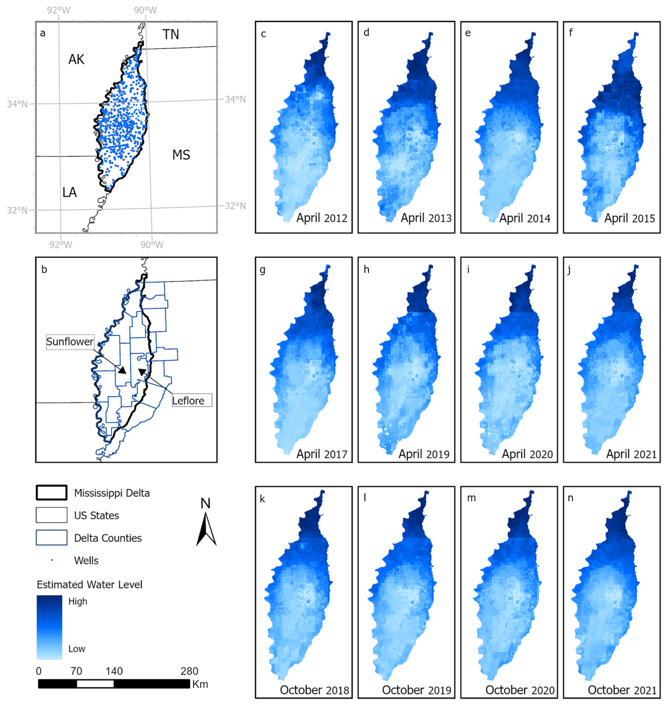
Accordingly, groundwater resources in the region are under significant stress, with over 90% of the supply being utilized for irrigation [14,23,30,31,32]. This intensive use has led to notable declines in water levels across parts of the aquifer [12]. According to [14], the potentiometric-surface map of the Delta region within the Mississippi Alluvial Plain reveals significant depressions. The most prominent depression occurs across the central Delta, between Leflore County to the west and Sunflower County to the east, directing water flow toward this area (Figure 1). Extensive groundwater extraction and surface water use for commercial production systems have been the primary drivers of this depression.

2.2. Materials

2.2.1. Precipitation and Temperature

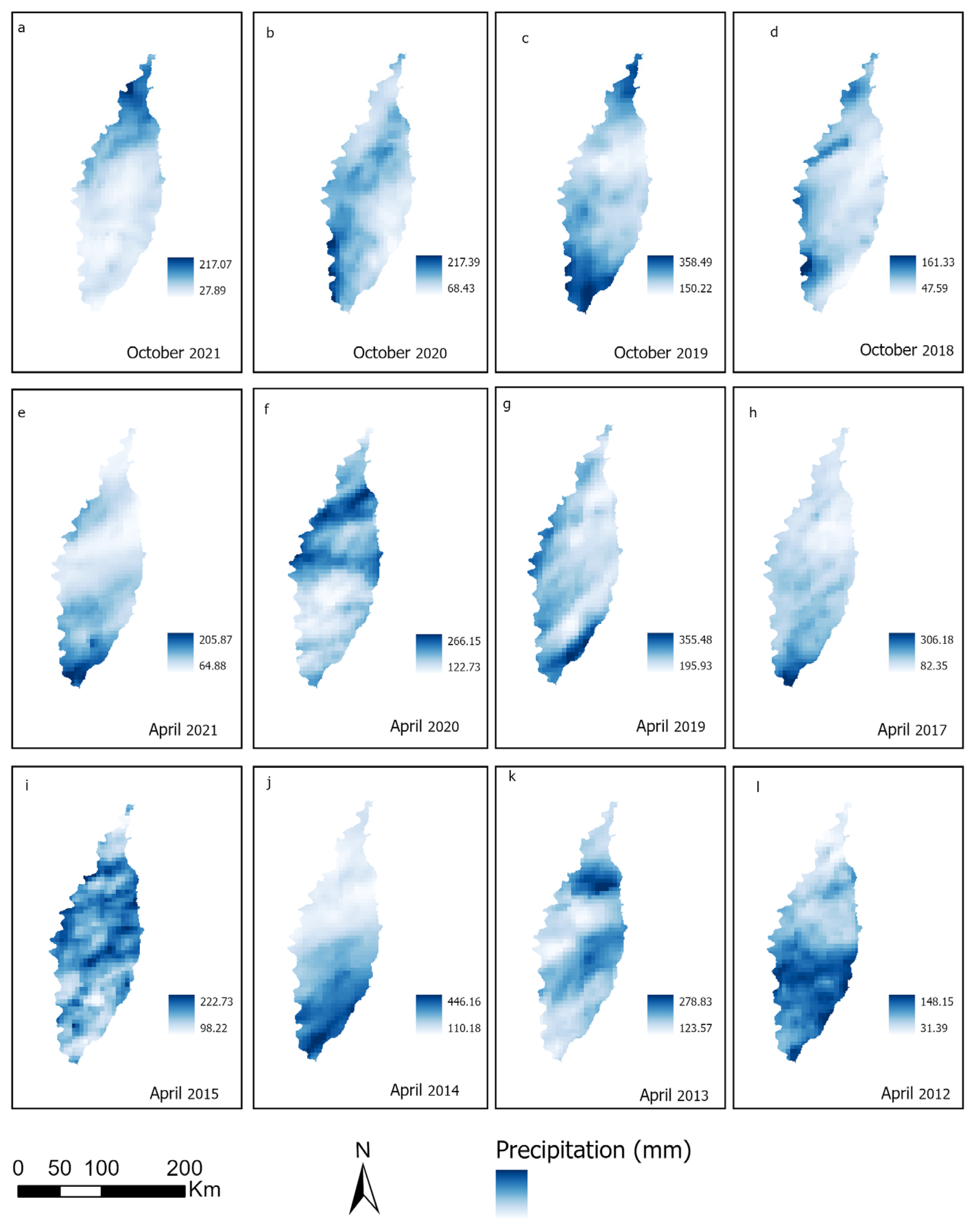
The data for precipitation and temperature were obtained from Parameter-elevation Regressions on Independent Slopes Model (PRISM) dataset for all months of 2012 to 2021. The data on PRISM dataset are available at ~4 km spatial resolution for free at daily and monthly temporal resolutions for the U.S. Dataset values are reported in the standard metric units [33]. Figure A1 and Figure A2 better show the temperature and precipitation pattern over the study area.

2.2.2. Aquifer Thickness

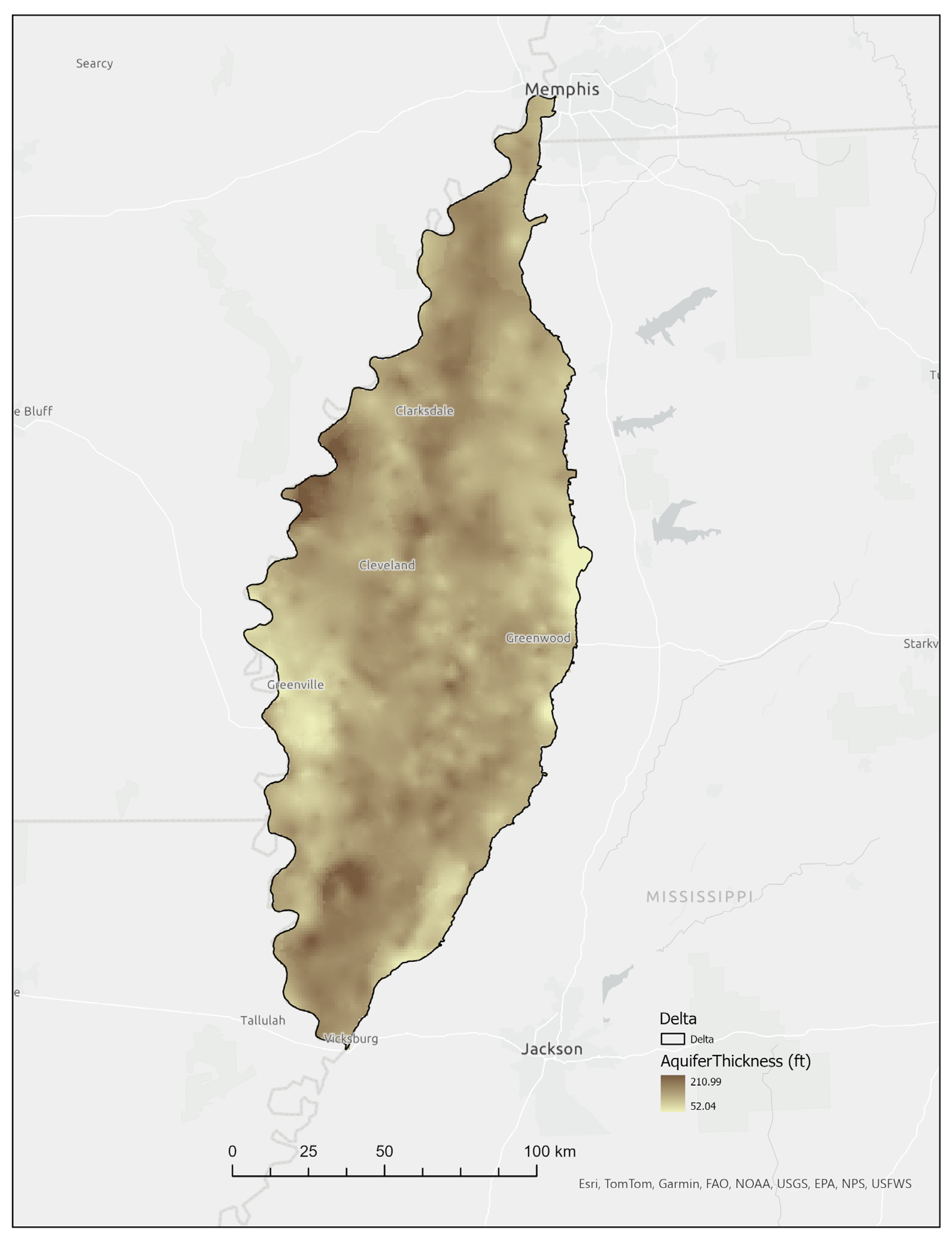
The raster data on the thickness of the Mississippi River Valley alluvial aquifer (MRVAA) were obtained from the U.S. Geological Survey (USGS) study, which estimates the bottom altitude and thickness of the Mississippi River Valley Alluvial Aquifer using geostatistical methods [34]. Covering a vast area in the southern U.S., the aquifer faces significant groundwater depletion due to irrigation demands [10]. This research integrates hydrogeologic data and statistical modeling to better define its structure, aiming to improve water resource management and inform geophysical surveys. Data supporting the study are available through a USGS release. More details are accessible at https://doi.org/10.5066/P9D9XR5F [34]. Figure A3 shows the aquifer thickness over Mississippi Delta.

2.2.3. NDVI

MODIS Vegetation Indices Monthly (MYD13C2) Version 6.1 product is the source of NDVI for our research. MYD13C2 is a globally cloud-free product with 0.05-degree spatial resolution and specifically focuses on the normalized difference vegetation index (NDVI) and enhanced vegetation index (EVI). NDVI is a commonly used metric to assess the health and vigor of vegetation. It measures the difference between the reflectance of near-infrared (NIR) and red light, indicating the density and vitality of vegetation. This product provides spatial and temporal information on vegetation conditions over large areas, on a 16-day composite basis. The MYD13C2 product includes several layers of information, such as NDVI values, EVI values, quality control flags, and pixel reliability information. We used “CMG 0.05 Deg Monthly NDVI” layer and multiplied it to its scale factor (0.0001) to obtain NDVI values ranging from −1 to +1 [35]. Figure A4 is the map of NDVI over years from the study area.

2.2.4. NLDAS Data

We used the North American Land Data Assimilation System (NLDAS) to obtain soil moisture and runoff data. NLDAS integrates various data sources, including weather observations and hydrological models, to provide high-resolution, gridded datasets for land surface states and fluxes across North America. It is widely used for hydrological and environmental studies due to its accuracy and temporal consistency, offering hourly and monthly data that support large-scale analyses of terrestrial water processes. We used NLDAS VIC Land Surface Model L4 Monthly 0.125 × 0.125-degree V002 data and obtained soil moisture content (SOILM), surface runoff (SSRUN), and plant canopy surface water (CNWAT). The unit of all of these products is kg/m3 [36,37].

2.2.5. GRACE/GRACE-FO

The GRACE and GRACE-FO satellite missions measure Earth’s gravitational field variations to monitor terrestrial water storage (TWS), including groundwater, soil moisture, surface waters, and snow and ice. GRACE operated from 2002 to 2017, succeeded by GRACE-FO in 2018. Using precise measurements, the missions detect mass changes with high accuracy, aiding global hydrology studies. We downloaded GRACE mascon products, the grids size of which is 0.5° after resampling from the original grid size of 3°.

2.2.6. In Situ Data

Wells data were provided by USGS and Yazoo Mississippi Delta Joint Water Management District (YMD) from 2008 to 2022. The USGS data contain 79 columns including wells’ ID, water level, altitude of water level, year, month, and day. We used the values in the column that report the actual altitude of the water level in feet, which we later converted to meters. The data from USGS are for all months of the year, with a significant reduction in data recorded from 2017 over the Mississippi Delta area. From 2017 to 2022, we used YMD data on wells for the Delta area. YMD conducts biannual monitoring in the Mississippi Delta, collecting water level data from over 400 wells during April and October. This monitoring captures fluctuations in groundwater levels before and after the irrigation season, offering valuable insights into regional dynamics. The distribution of wells over the study area is illustrated in Figure 1.

2.3. Methods

2.3.1. Random Forest

Random forest is a supervised, nonparametric ensemble learning method for classification and regression, introduced by [38]. It builds multiple decision trees using the CART algorithm, with randomness introduced by selecting different features at each node. Each tree is trained on a bootstrapped subset of the data, and predictions are aggregated for final outputs. The method evaluates the importance of input features by assessing the decrease in predictive accuracy when a feature’s values are randomly permuted, making it robust for diverse data applications.
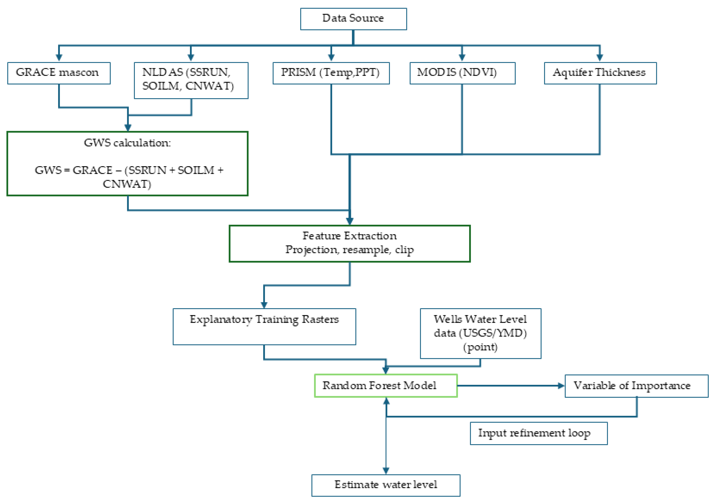
We used the “Forest-based and Boosted Classification and Regression” tool in ArcGIS Pro, which uses either the RF algorithm developed by [38] or extreme gradient boosting (XGBoost) algorithm developed by [39]. We chose the random forest algorithm and then chose the “predict to raster” method and selected each well’s layers for the months of April and October for the years 2012 to 2021 as “Input Training Feature” and selected the “actual altitude of the water level” as the “Variable to Predict”. Then, we added each layer of precipitation, temperature, ground water storage anomalies (GWSA), NDVI, and aquifer thickness as the “Explanatory Training Raster”. Then, we accepted the default setting for the number of trees (100), data available per tree (100%), and training data excluded for validation (10%).
While GRACE TWS and NLDAS soil moisture are physically meaningful hydrological variables, additional predictors such as aquifer thickness, precipitation, temperature, and NDVI were incorporated into the regression models as auxiliary variables due to their established influence on groundwater variability (e.g., [24,40,41]). Although these variables are not part of an explicit physical equation, they were included as input features in the machine learning models to enhance predictive performance. Their presence enables the model to capture nonlinear relationships and region-specific interactions between hydrological, climatic, and land surface conditions and groundwater storage (GWS). For instance, precipitation and temperature are recognized as key climatic drivers of groundwater recharge and depletion (e.g., [12,42]). Aquifer thickness, a static spatial variable, was included to account for the geological capacity for storing groundwater across the study area.

2.3.2. Data Preparation

After projecting the raster layers to the proper projection system (NAD 1983 UTM Zone 15N), we resampled them to 1 km cells and then clipped them to the Mississippi Delta borders.
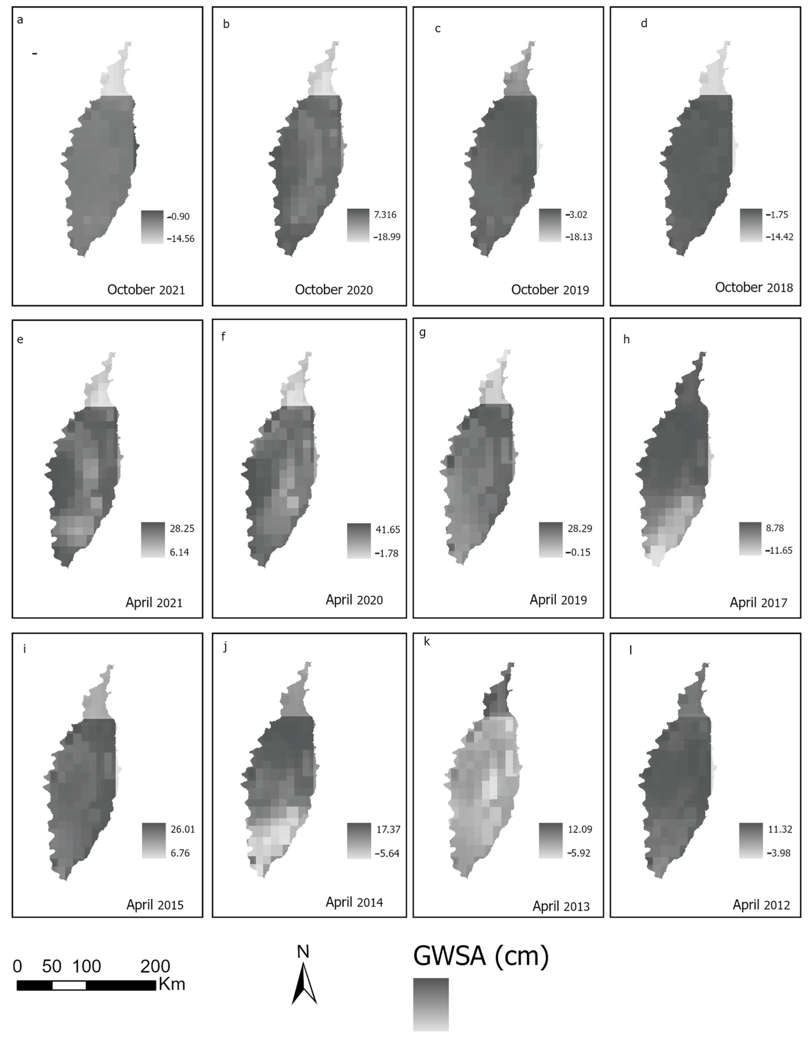
According to [43], to calculate the GWSA, we need to remove the different hydrological reservoirs anomalies, i.e., surface (∆WSurface water) and soil (∆WSoil water) waters, snow (∆WSnow), and groundwater (∆WGroundwater) from GRACE-based anomalies of TWS [43]. GWSA maps over the years for the study area can be found in Figure A5.
TWS = ∆WSurface water + ∆WSoil water + ∆WSnow + ∆WGroundwater,
Therefore, the GWSA is calculated as below:
∆WGroundwater = ∆TWS − (∆WSurface water + ∆WSoil water + ∆WSnow),
Since the water storage anomalies of GRACE are given in equivalent water thickness units in centimeter [16], the unit of all other parameters should be converted to the same unit as GRACE. For instance, the soil moisture content from NLDAS is reported as kg/m3. We used Equation (4) to convert the unit to cm:
1 [kg] of water at standard temperature and pressure = 1 [liter] = 1000 [cm3].
1 [m2] = 10,000 [cm2].
Therefore,
1 [kg/m2] of water = 1 [mm] = 0.1 [cm].
Therefore, we have aquifer thickness, temperature, precipitation, NDVI, and GWSA to use as the input of the model (Figure 2). We also should note that the GRACE data are missing for several months during its mission. For our study, the GRACE TWSA data are missing for April 2016 and 2018 and October 2012, 2015, 2016, and 2017. The GRACE & GRACE-FO Data Months/Days Table can be found at https://archive.podaac.earthdata.nasa.gov/podaac-ops-cumulus-docs/gracefo/open/docs/GRACE_GRACE-FO_Months_RL06.csv (accessed on 5 October 2023).

3. Results

After running the RF model to predict the water level for the MS Delta, for the months of April and October from 2012 to 2021, we obtained the results shown in Table 1. We report the R2, RMSE, and MAE statistical metrics to evaluate the predicted output of the RF model. A robust model has MAE and RMSE closer to 0 and R2 closer to 1.
As is shown in Table 1, R2 is very high (0.979 to 0.995) for the training data, suggesting the model fits the training data extremely well. MAE and RMSE values are relatively low in training (MAE: ~1.5–4.5 and RMSE: ~2.3–5.9), which means the model is learning the patterns in the training data with high precision and few errors. R2 in the validating dataset ranges from 0.879 to 0.984—still strong but slightly lower than in training, as expected. MAE and RMSE values are noticeably higher than in training: MAE: ~3.1–9.5; RMSE: ~4.0–13.2. This indicates that the model performs well but with some overfitting, especially in years like 2017, 2018, and 2019, where errors were greater in validation compared to training. Interestingly, extreme hydrological events included recorded flood and drought for all three years of 2017, 2018, and 2019. With the floods documented in “Weather.gov 2023” [44] and droughts in “Drought.Gov 2023” [45], we know that abnormal dry weather for April 2017 was experienced in around 46% for the state of Mississippi. According to Mississippi flood history, they recorded the longest known flood on record on the lower Mississippi river from 28 December 2018 through 10 August 2019. And there was also a flood event in March of 2018, which might be the reason for the higher RMSE and MAE in our model.
The R2 is high, which indicates that the model performs very well. There are more than 400 wells’ data recorded for each month of our study, which provides a useful data source for the model.
During training, 10% of the data were randomly excluded and set aside for validation purposes. This process, known as cross-validation, helps ensure that the model’s performance metrics—such as R2, MAE, and RMSE—accurately reflect its ability to predict groundwater levels on unseen data rather than just fitting the training data. By testing the model on this independent subset, we can evaluate its generalizability and robustness, minimizing the risk of overfitting and providing confidence that the model will perform well in real-world scenarios. This approach is particularly valuable in hydrological studies, where variability in environmental conditions can pose challenges for predictive accuracy [24].
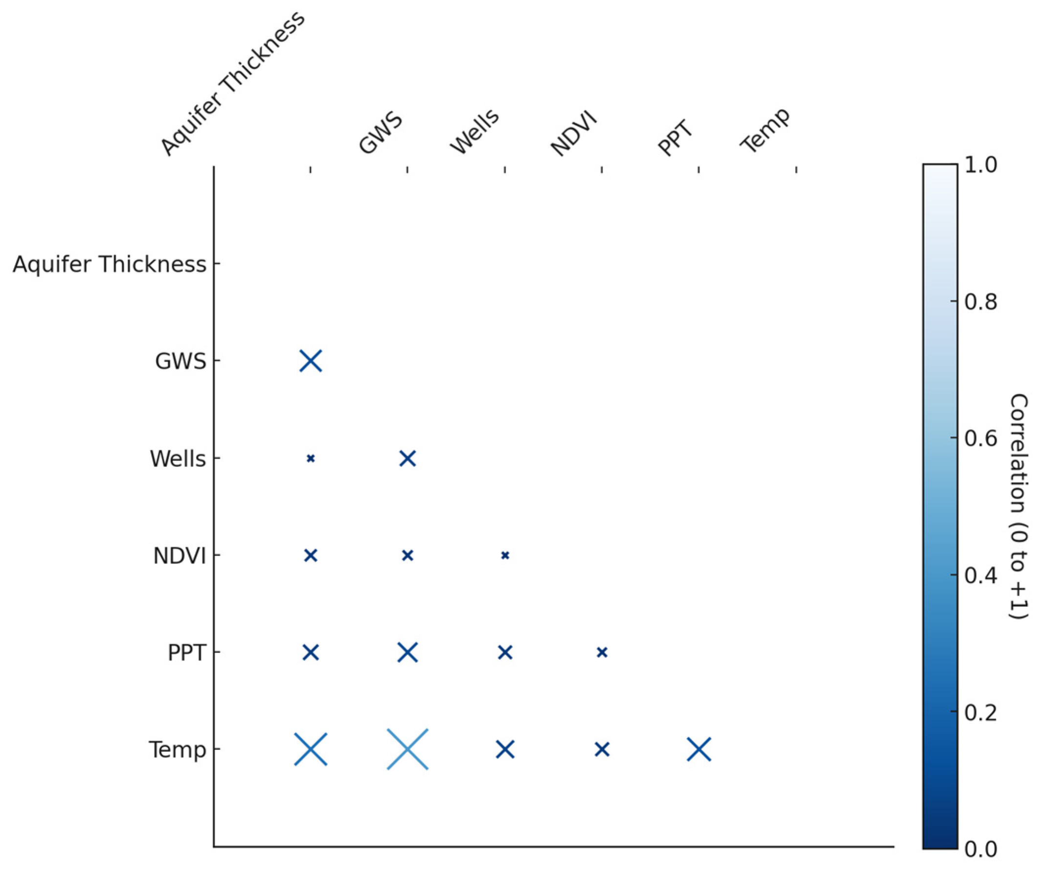
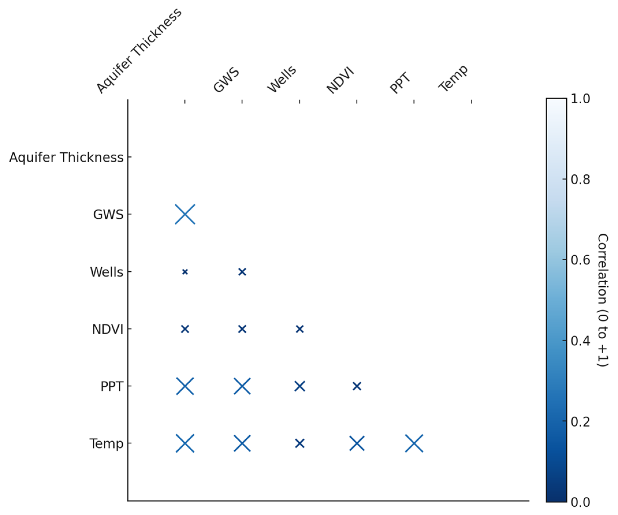
We created a scatterplot matrix to better understand the correlation between variables and if there is any multicollinearity present among the independent variables. Figure 3 and Figure 4 are the scatterplot matrix of the October and April data, respectively, over six years. Multicollinearity refers to high correlation among the independent (predictor) variables. High correlations can cause issues in regression models, such as unstable coefficient estimates. The correlations among the independent variables in Figure 3 and Figure 4 show that there are weak positive correlations among independent variables. Based on the values, there is no significant multicollinearity present among the independent variables in this dataset. All pairwise correlation coefficients are very low to weak. In summary, the independent variables appear to be largely uncorrelated with each other, which is a desirable characteristic for multiple regression analysis, as it helps ensure stable and interpretable regression coefficients. For the month of October, temperature shows the most correlation with wells’ data. And for the month of April, precipitation and temperature have the strongest (though still weak) correlations with wells’ data among this group. Similar to [40], the weak correlation between wells’ water level and precipitation may be due to a time lag in aquifer response to rainfall in April. The very weak correlation between precipitation and wells’ data in October might be due to less rainfall.
The model also shows the variable importance as a table, which indicates the significance of each variable in predicting the output of RF model. For the month of April, for 6 years, the temperature variable was the most important variable, followed by GWSA for 5 months. Precipitation was also an important variable in the model. For all months, NDVI and aquifer thickness rated as the least important variable. For the month of October, for six years, temperature was the most important variable, followed by GWSA for five months. Similar to the month of April, NDVI and aquifer thickness rated as the least important variables (See Table 2).
We observe significant year-to-year shifts in the importance of precipitation (PPT) for both April and October. For example, in April, PPT importance is notably high in 2012 (around 35%) and 2017 (around 23%). Correspondingly, 2012 experienced a moderate to severe drought and also had storm surge and flooding from Hurricane Isaac. In 2017, there were no significant droughts, but localized flash floods occurred. These extreme events would directly influence the importance of precipitation in the model. For October, PPT importance shows large swings (e.g., 15% in 2013 vs. 26% in 2020). The year 2020, with higher PPT importance, also experienced the Pearl River flood and multiple tropical storms (Cristobal, Delta, and Zeta), which would significantly alter precipitation’s role in groundwater dynamics.
Temperature (Temp) consistently appears as a highly important variable. The fluctuations here can be linked to temperature’s direct impact on groundwater recharge and discharge. High temperatures might accelerate evapotranspiration, reducing recharge. In drought years, higher temperatures can exacerbate water stress, making temperature a more critical predictor.
GWSA, as an indicator of antecedent conditions and extreme events, shows substantial variability, sometimes reaching very high importance (e.g., 35% in October 2019 and 35% in April 2019). This suggests that the antecedent groundwater conditions, influenced by past hydrological events, play a critical but fluctuating role. The massive Yazoo backwater flood in 2019, followed by multiple tropical storms in 2020, would directly impact overall groundwater storage. Therefore, the high importance of GWSA in these years strongly indicates that the long-term impacts of these major flood events on the overall water balance significantly influenced subsequent groundwater levels. In certain years, the existing water balance from previous months or seasons, heavily modified by floods or droughts, might be a stronger predictor of current groundwater levels than immediate climatic inputs.
NDVI and aquifer thickness generally show lower but still contributing importance. Their fluctuations, while less pronounced than Temp or PPT, may reflect the interannual variability in vegetation health (NDVI) due to climatic stress (e.g., drought years impacting vegetation, thereby affecting water uptake) or the baseline influence of aquifer geometry (aquifer thickness) in different hydrological contexts.
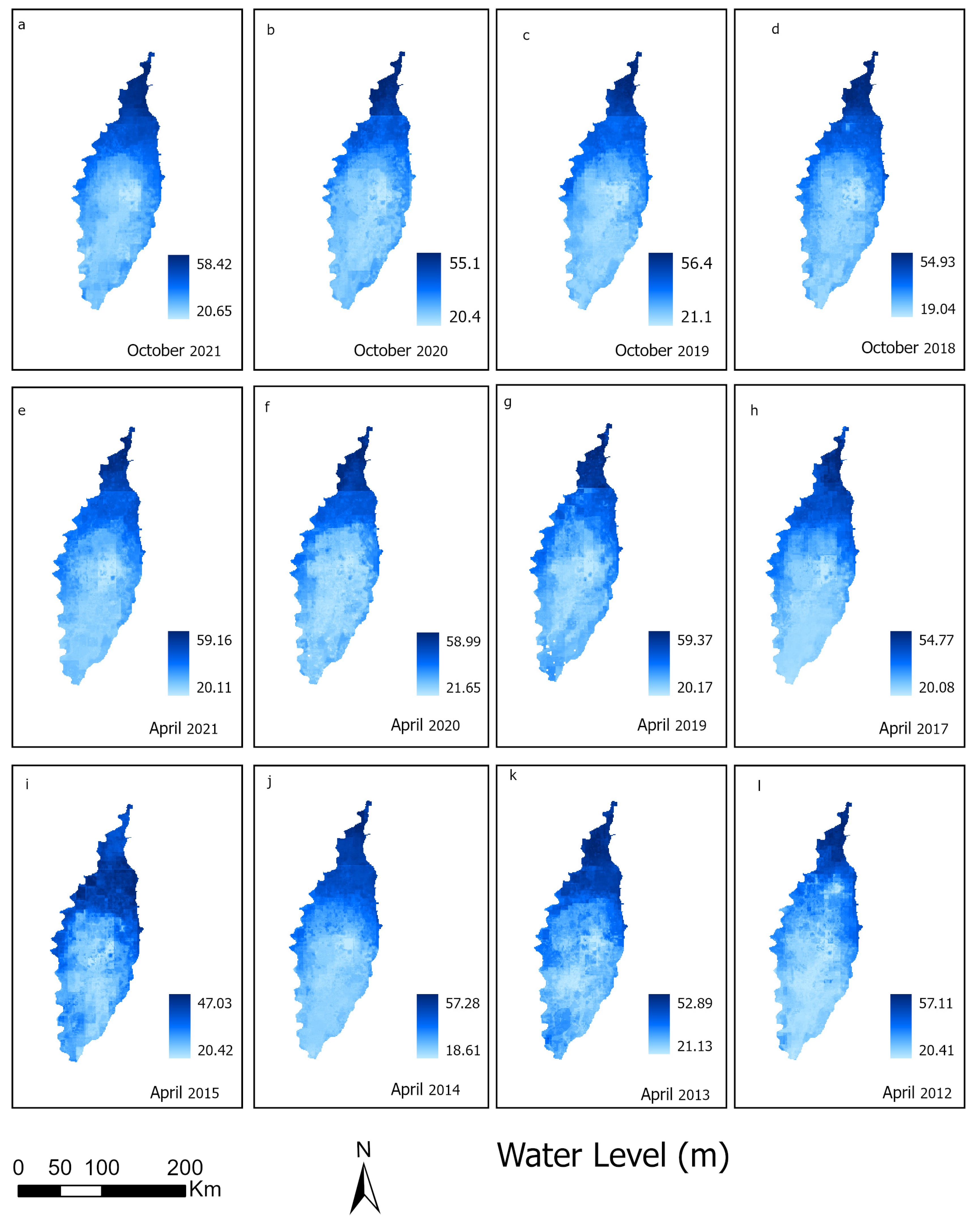
The output of the RF model is illustrated in Figure 5. As is shown in Figure 5c through 5n, the central region of the Delta (east of Sunflower and west of Leflore Counties) shows the lowest water level in all months through all years. The lowest value of water level for the month of April was 18.6 m during 2014, and the highest water level in 2019 was 59.37 m. October 2018 showed the lowest water level as 54.9 m, and October 2021’s 58.4 m water level was the highest value for the after-irrigation season period. The visualized result with quantitative legend may be found as Figure A6.
To further assess the accuracy of the model output, we calculated the difference between the model predictions and the corresponding in situ groundwater level measurements at each grid cell. The results of this comparison, including minimum, maximum, mean, standard deviation, and median of the differences—are now presented in Table 3. These statistics indicate that, despite the natural spatial heterogeneity of groundwater systems, the model closely approximates in situ observations, with mean differences near zero and moderate variability across the study period. This comparison reinforces the model’s ability to capture groundwater variability across a broad spatial domain, complementing the dense well network.
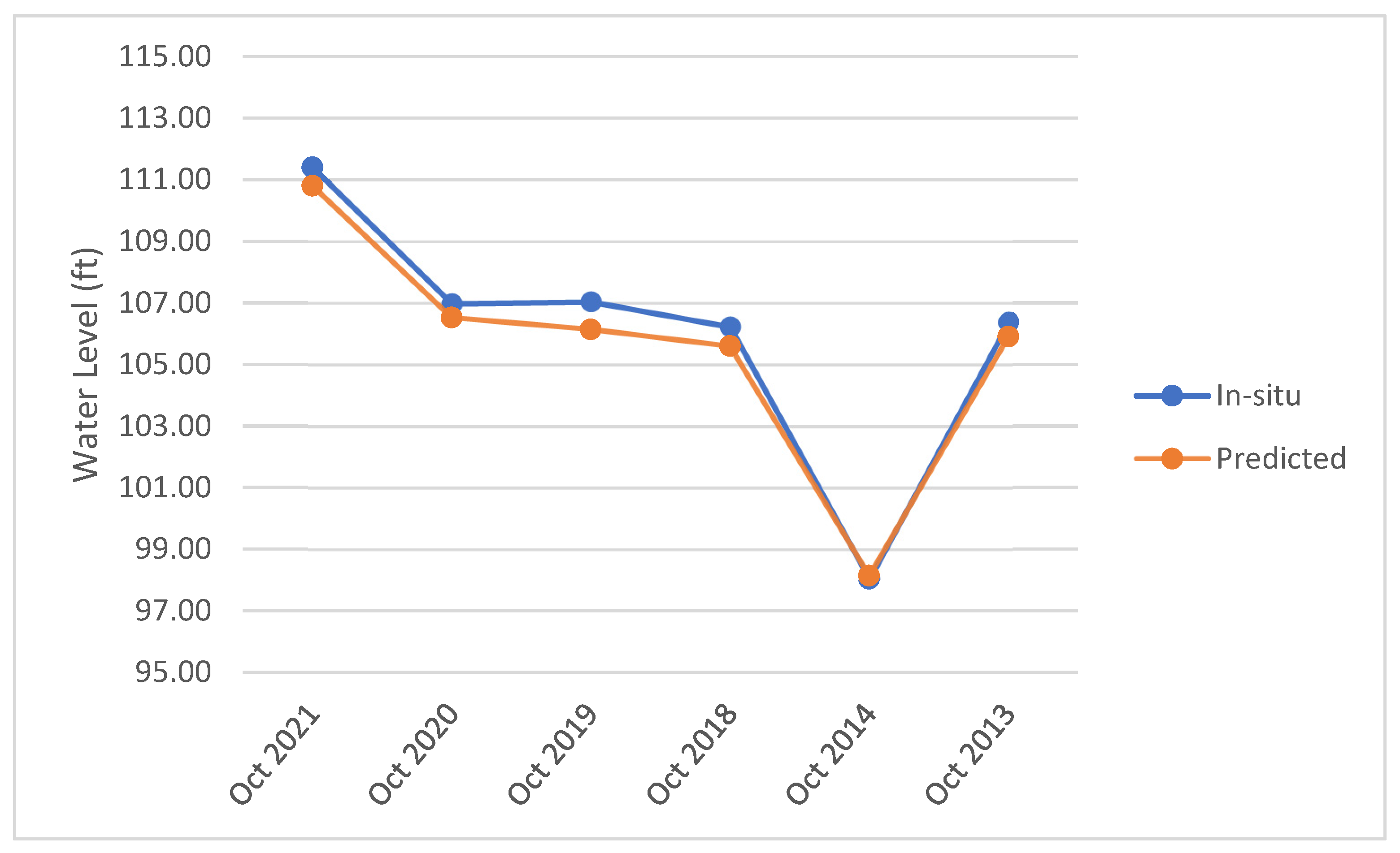
Figure 6 and Figure 7 also are visual comparison of the mean value of predicted and in situ water level for each grid cell containing wells. As it shows in both Figure 6 and Figure 7, the predicted water level is very close in all points to the observed wells’ water level.

4. Discussion

Our study demonstrates that the random forest model (RFM) performs exceptionally well in estimating groundwater levels in the study area. This finding is consistent with numerous studies that have employed RFM for downscaling GRACE-derived groundwater storage anomalies (GWSA). Unlike studies such as [21], which compare RFM with alternative models, our research focused solely on RFM’s ability to downscale GWSA and estimate groundwater levels. However, a review of the literature suggests that RFM consistently outperforms other models in similar applications. Several studies across different geographic regions [19,21,24,25,40,46] report higher R2 values for RFM compared to other machine learning models, highlighting its robustness in capturing complex relationships between groundwater levels and predictor variables. This consistency suggests that RFM is a reliable approach for downscaling GRACE products on a global scale [47].
The strong performance of RFM in estimating groundwater levels where well data are available has significant implications for water resource management. By improving the spatial and temporal resolution of groundwater estimates, RFM enables researchers and policymakers to make more informed decisions regarding water availability, drought monitoring, and sustainable groundwater extraction. The model’s reliance on satellite-based inputs enhances its applicability across diverse regions, particularly where in situ groundwater measurements are sparse. However, input variables may need to be tailored to specific study areas; for example, topography could play a more significant role in regions with steep terrain. Additionally, exploring RFM’s potential for long-term groundwater forecasting could enhance its utility in predicting future water availability under changing climatic conditions.
While our study demonstrates the effectiveness of RFM, it is important to acknowledge potential limitations:
1
The model’s performance may vary in regions with limited ground-truth data for validation;
2
Extreme hydrological events or long-term climate change impacts could affect model performance, which should be considered in future scenarios;
3
Further investigation is required to assess the model’s applicability in regions with significantly different hydrogeological conditions.
Addressing these limitations in future research will further enhance the applicability and reliability of RFM in groundwater level estimation.

5. Conclusions

Accurately detecting groundwater storage is crucial for effective and sustainable water resource management, particularly in regions where agriculture and other water-intensive activities heavily depend on groundwater availability. For farmers and stakeholders who rely on groundwater for irrigation, there is a growing need for efficient and cost-effective tools that can provide reliable, local-scale groundwater information to support sustainable crop production amid ongoing depletion [47]. Reliable access to precise data is key to informed decision making, yet spatial and temporal limitations in measuring in situ groundwater levels present a significant barrier [12]. This study demonstrates that incorporating random forest modeling (RFM) with satellite-based observations, such as GRACE data, provides a robust and accurate method for estimating groundwater levels. Specifically, for the Mississippi Delta, our approach yielded high accuracy in capturing groundwater trends and dynamics. Our model’s primary purpose is to estimate groundwater levels in areas lacking in situ measurements, by leveraging remote sensing and environmental inputs. This spatial estimation capability is particularly valuable for supporting agricultural decision making, where access to accurate groundwater information can inform water management strategies and crop selection in data-scarce regions.
The results of this study align closely with the U.S. Geological Survey (USGS) potentiometric-surface report for the Delta [48], confirming groundwater level depressions in central areas of the Delta that are likely exacerbated by intensive production water withdrawals. Although broad spatial patterns are consistent among our and USGS methods, even minor model changes can reveal important differences toward agroecological and hydrologic relationships [13]. By successfully downscaling the time-series of GRACE products, our research provides a fine-scale understanding of groundwater fluctuations for both pre- and post-irrigation seasons in the Mississippi Delta.
The implications of this study are significant, as it provides an advanced tool for improving water management strategies in the region. The insights derived from this research can help policymakers and stakeholders better manage the Delta’s groundwater resources, fostering sustainable production systems while minimizing the risks of groundwater depletion. Access to accurate, high-resolution, and continuous groundwater data enabled by this approach could support adaptive management practices and improve resilience in water-scarce regions. Furthermore, this methodology may serve as a model for other regions facing similar challenges, highlighting the potential of integrating machine learning with satellite data for groundwater monitoring and management worldwide.

Author Contributions

Conceptualization, G.E., L.D.Y. and Z.G.; methodology, Z.G.; software, Z.G. and A.R.A.; resources, G.E. and L.D.Y.; writing—original draft preparation, Z.G.; writing—review and editing, Z.G., A.R.A. and L.J.H.; visualization, Z.G.; supervision, G.E. and L.D.Y.; funding acquisition, G.E. and L.D.Y. All authors have read and agreed to the published version of the manuscript.

Funding

This work was funded by a research grant awarded by the National Science Foundation (Award no: OIA 2019561) and U.S. Geological Survey under Grant/Cooperative Agreement No. G23AP00683 and was supported by USDA-ARS Project # 6060–13660-009-00D.

Institutional Review Board Statement

Not applicable.

Informed Consent Statement

Not applicable.

Data Availability Statement

Existing well location and associated water levels datasets from The Yazoo–Mississippi Delta Joint Water-Management District are available through https://www.ymd.org/ (accessed on 10 January 2024). The water level data for the aquifer can be found at National Water Information System (NWIS)—USGS Water Data for the Nation. Temperature and Precipitation data were derived from PRISM weather data (https://prism.oregonstate.edu/, accessed on 10 January 2024). MODIS NDVI data were obtained from NASA EARTHDATA website at https://www.earthdata.nasa.gov/data/catalog/lpcloud-myd13c2-006 (accessed on 10 January 2024). NLDAS data were derived from NASA EARTHDATA website at: https://disc.gsfc.nasa.gov/datasets?keywords=NLDAS (accessed on 10 January 2024).

Acknowledgments

We thank the Yazoo–Mississippi Delta Joint Water-Management District for providing data on well locations and associated water levels. We sincerely appreciate Mohammad Al-Hamdan and Jiayu Fang from the National Center for Computational Hydroscience and Engineering (NCCHE) at the University of Mississippi for their guidance on the use, collection, and description of NLDAS data for this paper. We also thank Wade Kress and Anna M. Nottmeier, both from the United States Geological Survey, for their assistance with the National Water Information System. We also gratefully acknowledge Pushpendra Raghav for his guidance and valuable input on the MODIS data. Mention of trade names or commercial products in this publication is solely for the purpose of providing specific information and does not imply recommendation or endorsement by the U.S. Department of Agriculture. USDA is an equal opportunity provider, employer, and lender.

Conflicts of Interest

The authors declare no conflicts of interest.

Appendix A

Figure A1. Temperature for the Delta for October and April for selected years from 2012 to 2021. (al) Time series of temperature in Mississippi Delta for selected month and years from 2012 to 2021.
Limnolrev 25 00039 g0a1
Figure A2. Precipitation for the Delta for October and April for selected years from 2012 to 2021. (al) Time series of precipitation in Mississippi Delta for selected month and years from 2012 to 2021.
Limnolrev 25 00039 g0a2
Figure A3. Aquifer thickness over the Delta.
Limnolrev 25 00039 g0a3
Figure A4. NDVI for the Delta for October and April for selected years from 2012 to 2021. (al) Time series of NDVI in Mississippi Delta for selected month and years from 2012 to 2021.
Limnolrev 25 00039 g0a4
Figure A5. GWSA for the Delta for October and April for selected years from 2012 to 2021. (al) Time series of GWSA in Mississippi Delta for selected month and years from 2012 to 2021.
Limnolrev 25 00039 g0a5
Figure A6. Estimated water level for the Delta for October and April (before and after irrigation season) for selected years from 2012 to 2021. The legend for each map is provided in meters. (al) Time series of model estimated water level in Mississippi Delta for selected month and years from 2012 to 2021.
Limnolrev 25 00039 g0a6

References

  1. Konikow, L. Long-Term Groundwater Depletion in the United States. Groundwater 2015, 53, 2–9. [Google Scholar] [CrossRef]
  2. Scanlon, B.R.; Rateb, A.; Pool, D.R.; Sanford, W.; Save, H.; Sun, A.; Long, D.; Fuchs, B. Effects of Climate and Irrigation on GRACE-Based Estimates of Water Storage Changes in Major US Aquifers. Environ. Res. Lett. 2021, 16, 094009. [Google Scholar] [CrossRef]
  3. Zhang, J.; Liu, K.; Wang, M. Downscaling Groundwater Storage Data in China to a 1-Km Resolution Using Machine Learning Methods. Remote Sens. 2021, 13, 523. [Google Scholar] [CrossRef]
  4. Gonzalez, R.Q.; Arsanjani, J.J. Prediction of Groundwater Level Variations in a Changing Climate: A Danish Case Study. ISPRS Int. J. Geo-Inf. 2021, 10, 792. [Google Scholar] [CrossRef]
  5. Mehta, P.; Siebert, S.; Kummu, M.; Deng, Q.; Ali, T.; Marston, L.; Xie, W.; Davis, K.F. Half of Twenty-First Century Global Irrigation Expansion Has Been in Water-Stressed Regions. Nat. Water 2024, 2, 254–261. [Google Scholar] [CrossRef]
  6. Mekonnen, M.M.; Hoekstra, A.Y. A Global Assessment of the Water Footprint of Farm Animal Products. Ecosystems 2012, 15, 401–415. [Google Scholar] [CrossRef]
  7. Tao, H.; Hameed, M.M.; Marhoon, H.A.; Zounemat-Kermani, M.; Heddam, S.; Kim, S.; Sulaiman, S.O.; Tan, M.L.; Sa’adi, Z.; Mehr, A.D.; et al. Groundwater Level Prediction Using Machine Learning Models: A Comprehensive Review. Neurocomputing 2022, 489, 271–308. [Google Scholar] [CrossRef]
  8. Warziniack, T.; Arabi, M.; Brown, T.C.; Froemke, P.; Ghosh, R.; Rasmussen, S.; Swartzentruber, R. Projections of Freshwater Use in the United States Under Climate Change. Earths Future 2022, 10, e2021EF002222. [Google Scholar] [CrossRef]
  9. USDA-NASS. 2018 Irrigation and Water Management Survey; Special Studies, Part 1. AC-17-SS-1; USDA National Agricultural Statistics Service (NASS): Harrisburg, PA, USA, 2019.
  10. Lovelace, J.K.; Nielsen, M.G.; Read, A.L.; Murphy, C.L.; Maupin, M.A. Estimated Groundwater Withdrawals from Principal Aquifers in the United States, 2015; Circular; U.S. Geological Survey: Reston, VA, USA, 2020.
  11. Nourani, V.; Jabbarian Paknezhad, N.; Ng, A.; Wen, Z.; Dabrowska, D.; Üzelaltınbulat, S. Application of the Machine Learning Methods for GRACE Data Based Groundwater Modeling, a Systematic Review. Groundw. Sustain. Dev. 2024, 25, 101113. [Google Scholar] [CrossRef]
  12. Ghaffari, Z.; Easson, G.; Yarbrough, L.D.; Awawdeh, A.R.; Jahan, M.N.; Ellepola, A. Using Downscaled GRACE Mascon Data to Assess Total Water Storage in Mississippi Alluvial Plain Aquifer. Sensors 2023, 23, 6428. [Google Scholar] [CrossRef]
  13. Heintzman, L.J.; Ghaffari, Z.; Awawdeh, A.R.; Barrett, D.E.; Yarbrough, L.D.; Easson, G.; Moore, M.T.; Locke, M.A.; Yasarer, H.I. Assessing Differences in Groundwater Hydrology Dynamics Between In Situ Measurements and GRACE-Derived Estimates via Machine Learning: A Test Case of Consequences for Agroecological Relationships Within the Yazoo–Mississippi Delta (USA). Hydrology 2024, 11, 186. [Google Scholar] [CrossRef]
  14. McGuire, V.L.; Seanor, R.C.; Asquith, W.H.; Nottmeier, A.M.; David, S.C.; Tollett, R.W.; Kress, W.H.; Strauch, K.R. Datasets Used to Map the Potentiometric Surface, Mississippi River Valley Alluvial Aquifer, Spring 2020. In Scientific Investigations Map; U.S. Geological Survey: Reston, VA, USA, 2021. [Google Scholar]
  15. Yasarer, L.M.W.; Taylor, J.M.; Rigby, J.R.; Locke, M.A. Trends in Land Use, Irrigation, and Streamflow Alteration in the Mississippi River Alluvial Plain. Front. Environ. Sci. 2020, 8, 66. [Google Scholar] [CrossRef]
  16. JPL. Level-3 Data Product User Handbook, Revision 1. In Gravity Recovery and Climate Experiment––Follow-on. (GRACE-FO); D-103133; Jet Propulsion Laboratory, California Institute of Technology: Pasadena, CA, USA, 2019. [Google Scholar]
  17. Sneeuw, N.; Vishwakarma, B.D.; Zhang, J. Statistical downscaling of GRACE products to improve spatial resolution. In Proceedings of the EGU General Assembly 2021, Online, 19–30 April 2021. EGU21-10022. [Google Scholar] [CrossRef]
  18. Vishwakarma, B.D.; Zhang, J.; Sneeuw, N. Downscaling GRACE Total Water Storage Change Using Partial Least Squares Regression. Sci. Data 2021, 8, 95. [Google Scholar] [CrossRef] [PubMed]
  19. Tao, H.; Al-Sulttani, A.H.; Salih, S.Q.; Mohammed, M.K.A.; Khan, M.A.; Beyaztas, B.H.; Ali, M.; Elsayed, S.; Shahid, S.; Yaseen, Z.M. Development of High-Resolution Gridded Data for Water Availability Identification through GRACE Data Downscaling: Development of Machine Learning Models. Atmospheric Res. 2023, 291, 106815. [Google Scholar] [CrossRef]
  20. Ali, S.; Ran, J.; Khorrami, B.; Wu, H.; Tariq, A.; Jehanzaib, M.; Khan, M.M.; Faisal, M. Downscaled GRACE/GRACE-FO Observations for Spatial and Temporal Monitoring of Groundwater Storage Variations at the Local Scale Using Machine Learning. Groundw. Sustain. Dev. 2024, 25, 101100. [Google Scholar] [CrossRef]
  21. Jyolsna, P.J.; Kambhammettu, B.V.N.P.; Gorugantula, S. Application of Random Forest and Multi-Linear Regression Methods in Downscaling GRACE Derived Groundwater Storage Changes. Hydrol. Sci. J. 2021, 66, 874–887. [Google Scholar] [CrossRef]
  22. Verma, K.; Katpatal, Y.B. Groundwater Monitoring Using GRACE and GLDAS Data after Downscaling Within Basaltic Aquifer System. Groundwater 2020, 58, 143–151. [Google Scholar] [CrossRef]
  23. Awawdeh, A.R.M.; Yasarer, H.; Ghaffari, Z.; Yarbrough, L.D. Downscaling GRACE Data for Improved Groundwater Forecasting Using Artificial Neural Networks. Civ. Eng. J. 2025, 11, 406–419. [Google Scholar] [CrossRef]
  24. Chen, L.; He, Q.; Liu, K.; Li, J.; Jing, C. Downscaling of GRACE-Derived Groundwater Storage Based on the Random Forest Model. Remote Sens. 2019, 11, 2979. [Google Scholar] [CrossRef]
  25. Sabzehee, F.; Amiri-Simkooei, A.R.; Iran-Pour, S.; Vishwakarma, B.D.; Kerachian, R. Enhancing Spatial Resolution of GRACE-Derived Groundwater Storage Anomalies in Urmia Catchment Using Machine Learning Downscaling Methods. J. Environ. Manage. 2023, 330, 117180. [Google Scholar] [CrossRef] [PubMed]
  26. Ladd, D.E.; Travers, L.R. Generalized Regions of the Mississippi Alluvial Plain; U.S. Geological Survey: Reston, VA, USA, 2019.
  27. Omernik, J.M. Ecoregions of the Conterminous United States. Ann. Assoc. Am. Geogr. 1987, 77, 118–125. [Google Scholar] [CrossRef]
  28. Omernik, J.M.; Griffith, G.E. Ecoregions of the Conterminous United States: Evolution of a Hierarchical Spatial Framework. Environ. Manag. 2014, 54, 1249–1266. [Google Scholar] [CrossRef] [PubMed]
  29. Heintzman, L.J.; McIntyre, N.E.; Langendoen, E.J.; Read, Q.D. Cultivation and Dynamic Cropping Processes Impart Land-Cover Heterogeneity within Agroecosystems: A Metrics-Based Case Study in the Yazoo-Mississippi Delta (USA). Landsc. Ecol. 2024, 39, 29. [Google Scholar] [CrossRef]
  30. Arthur, J. Hydrogeology, Model Description, and Flow Analysis of the Mississippi River Alluvial Aquifer in Northwestern Mississippi; Water-Resources Investigations Report; USGS: Jackson, MS, USA, 2001.
  31. Barlow, J.R.B.; Clark, B.R. Simulation of Water-Use Conservation Scenarios for the Mississippi Delta Using an Existing Regional Groun water Flow Model; U.S. Geological Survey, Scientific Investigations Report; USGS: Jackson, MS, USA, 2011.
  32. Killian, C.D.; Asquith, W.H.; Barlow, J.R.B.; Bent, G.C.; Kress, W.H.; Barlow, P.M.; Schmitz, D.W. Characterizing Groundwater and Surface-Water Interaction Using Hydrograph-Separation Techniques and Groundwater-Level Data throughout the Mississippi Delta, USA. Hydrogeol. J. 2019, 27, 2167–2179. [Google Scholar] [CrossRef]
  33. PRISM Climate Group, Oregon State University. Available online: https://prism.oregonstate.edu (accessed on 19 April 2022).
  34. Torak, L.J.; Painter, J.A. Digital Surfaces of the Bottom Altitude and Thickness of the Mississippi River Valley Alluvial Aquifer and Site Data within the Mississippi Alluvial Plain Project Region; U.S. Geological Survey Data Release; USGS: Jackson, MS, USA, 2019.
  35. Didan, K. MODIS/Aqua Vegetation Indices Monthly L3 Global 1 km SIN Grid V061 2021. Available online: https://www.earthdata.nasa.gov/data/catalog/lpcloud-myd13a3-061 (accessed on 10 January 2024).
  36. Mocko, D. NASA/GSFC/HSL NLDAS Mosaic Land Surface Model L4 Monthly 0.125 x 0.125 Degree, Version 002 2012. Available online: https://cmr.earthdata.nasa.gov/search/concepts/C1887990159-GES_DISC.html (accessed on 24 January 2024).
  37. Mocko, D. NASA/GSFC/HSL NLDAS VIC Land Surface Model L4 Monthly 0.125 x 0.125 Degree, Version 002 2014. Available online: https://cmr.earthdata.nasa.gov/search/concepts/C1887583680-GES_DISC.html (accessed on 24 January 2024). [CrossRef]
  38. Breiman, L. Random Forests. Mach. Learn. 2001, 45, 5–32. [Google Scholar] [CrossRef]
  39. Chen, T.; Guestrin, C. XGBoost: A Scalable Tree Boosting System. In Proceedings of the 22nd ACM SIGKDD International Conference on Knowledge Discovery and Data Mining, San Francisco, CA, USA, 13–17 August 2016; ACM: New York, NY, USA, 2016; pp. 785–794. [Google Scholar]
  40. Ali, S.; Liu, D.; Fu, Q.; Cheema, M.J.M.; Pham, Q.B.; Rahaman, M.M.; Dang, T.D.; Anh, D.T. Improving the Resolution of GRACE Data for Spatio-Temporal Groundwater Storage Assessment. Remote Sens. 2021, 13, 3513. [Google Scholar] [CrossRef]
  41. Miro, M.; Famiglietti, J. Downscaling GRACE Remote Sensing Datasets to High-Resolution Groundwater Storage Change Maps of California’s Central Valley. Remote Sens. 2018, 10, 143. [Google Scholar] [CrossRef]
  42. Khorrami, B.; Gunduz, O. Evaluation of the Temporal Variations of Groundwater Storage and Its Interactions with Climatic Variables Using GRACE Data and Hydrological Models: A Study from Turkey. Hydrol. Process. 2021, 35, e14076. [Google Scholar] [CrossRef]
  43. Frappart, F.; Ramillien, G. Monitoring Groundwater Storage Changes Using the Gravity Recovery and Climate Experiment (GRACE) Satellite Mission: A Review. Remote Sens. 2018, 10, 829. [Google Scholar] [CrossRef]
  44. US Department of Commerce. Mississippi River Flood History 1543-Present. National Weather Service; National Oceanic and Atmospheric Administration, US Department of Commerce: New Orleans, LA, USA, 2023.
  45. National Integrated Drought Information System. Historical Data and Conditions. 1315 East-West Highway Silver Spring, United States. 2025. Available online: https://www.drought.gov/historical-information (accessed on 1 January 2025).
  46. Chen, Z.; Zheng, W.; Yin, W.; Li, X.; Zhang, G.; Zhang, J. Improving the Spatial Resolution of GRACE-Derived Terrestrial Water Storage Changes in Small Areas Using the Machine Learning Spatial Downscaling Method. Remote Sens. 2021, 13, 4760. [Google Scholar] [CrossRef]
  47. Guzman, S.M.; Paz, J.O.; Tagert, M.L.M.; Mercer, A.E. Evaluation of Seasonally Classified Inputs for the Prediction of Daily Groundwater Levels: NARX Networks Vs Support Vector Machines. Environ. Model. Assess. 2019, 24, 223–234. [Google Scholar] [CrossRef]
  48. McGuire, V.L.; Seanor, R.C.; Asquith, W.H.; Strauch, K.R.; Nottmeier, A.M.; Thomas, J.C.; Tollett, R.W.; Kress, W.H. Altitude of the Potentiometric Surface in the Mississippi River Valley Alluvial Aquifer, Spring 2020; U.S. Geological Survey, Scientific Investigation Map; USGS: Jackson, MS, USA, 2021.
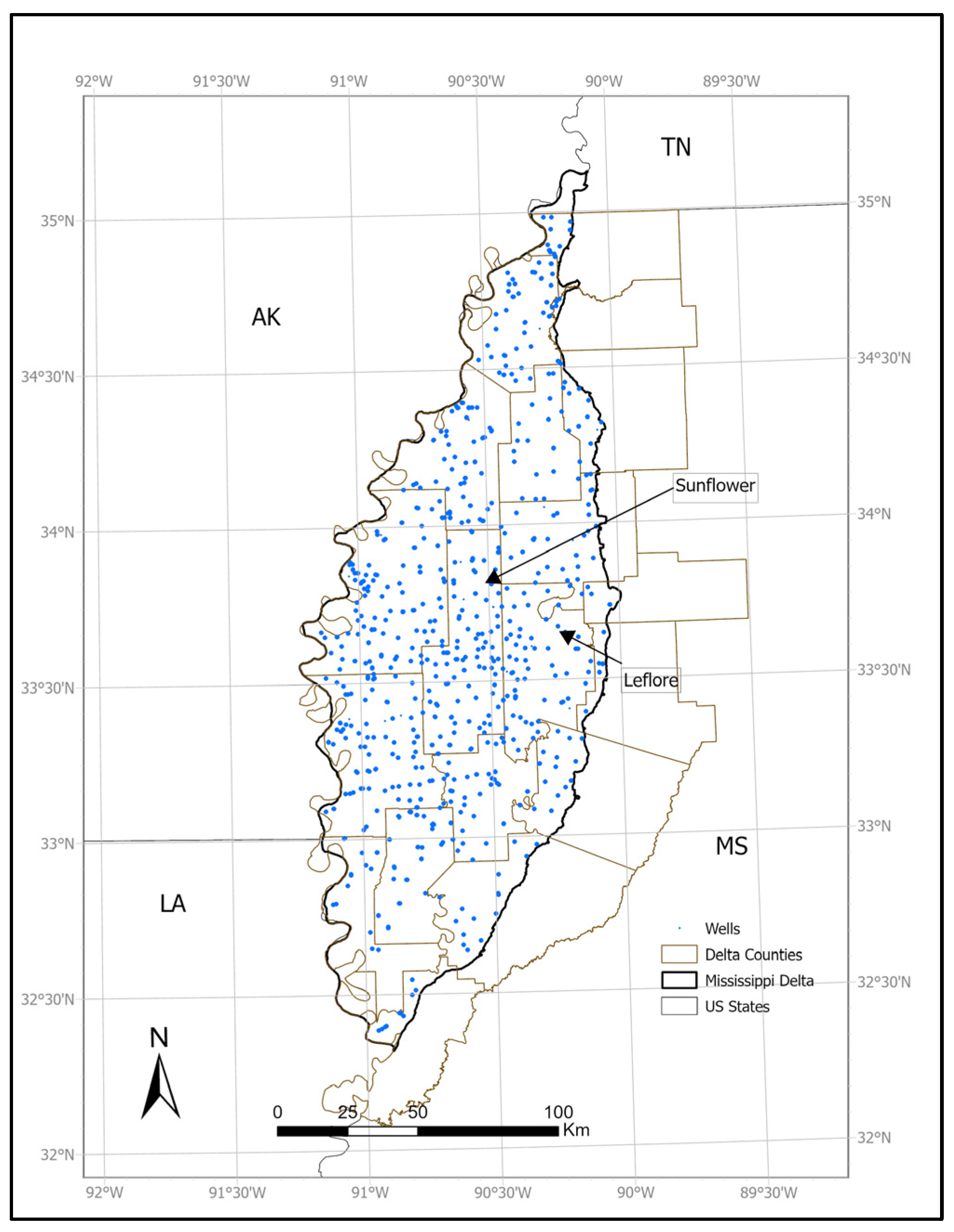
Figure 1. Study area and the wells within the study area.
Limnolrev 25 00039 g001
Figure 2. Methodological workflow of research.
Limnolrev 25 00039 g002
Figure 3. Scatterplot matrix for the variables for October. Larger “X” shows higher correlation.
Limnolrev 25 00039 g003
Figure 4. Scatterplot matrix for the variables for April. Larger “X” shows higher correlation.
Limnolrev 25 00039 g004
Figure 5. Estimated water level for Delta for October and April (before and after irrigation season) for selected years from 2012 to 2021. (a) shows the study area and the observational wells; (b) counties within the Mississippi Delta; emphasizing Sunflower and Leflore counties which had reported water depletion in USGS report; (cn) Time series of estimated water level in Mississippi Delta for selected month and years from 2012 to 2021.
Limnolrev 25 00039 g005
Figure 6. Comparison of observed and predicted water level for wells in October of several years.
Limnolrev 25 00039 g006
Figure 7. Comparison of observed and predicted water level for wells in April of several years.
Limnolrev 25 00039 g007
Table 1. Statistical metrics summary of RF for MAP for April and October.
MonthYearTraining DataValidation Data
April R2MAERMSER2MAERMSE
20120.9892.6323.7310.9515.7628.289
20130.9892.2892.9540.9365.2627.658
20140.9941.9482.6740.9653.7815.045
20150.9921.9832.6510.9763.2634.825
20170.9823.4344.6560.9249.47313.164
20190.9794.5955.8980.9179.04411.244
20200.9814.0675.4230.9057.79610.144
20210.9843.5994.6160.9257.3039.143
October20130.9951.7262.3850.9843.094.028
20140.9941.5562.3130.9823.6294.523
20180.9853.1934.3890.8798.05310.881
20190.983.564.8460.9555.6527.874
20200.9883.0874.1370.9326.8019.308
20210.9823.4784.5150.9427.0229.055
Table 2. Variable Importance Table.
Top Variable Importance (%)
MonthYear201220132014201520172018201920202021
AprilVariable
Temperature3244353944-334039
Precipitation3613311423-111317
NDVI7108107-1088
GWSA1621192413-352827
Aquifer Thickness10128128-111010
OctoberTemperature-4440--46413833
Precipitation-1511--1115826
NDVI-1015--118139
GWSA-2519--24273225
Aquifer Thickness-615--81086
Table 3. Comparison of in situ and predicted water level over pixels that have well(s) inside.
MonthYearMinMaxMeanStd. Dev.Median
April2012−35.6138.740.218.33−0.55
2013−33.0231.74−0.226.42−0.49
2014−19.9427.70.15.82−0.22
2015−24.2321.83−0.215.47−0.2
2017−21.5245.260.437.67−0.25
2019−23.5646.320.0538.71−0.72
2020−25.0520.52−0.427.86−0.83
2021−20.5225.950.197.08−0.69
October2013−21.1522.92−0.315.44−0.36
2014−13.8822.81−0.395.04−0.41
2018−26.9240.640.166.87−0.55
2019−18.3124.090.2676.740.205
2020−22.9628.39−0.147−6.49−0.85
2021−23.2723.20.0276.54−4.484
Disclaimer/Publisher’s Note: The statements, opinions and data contained in all publications are solely those of the individual author(s) and contributor(s) and not of MDPI and/or the editor(s). MDPI and/or the editor(s) disclaim responsibility for any injury to people or property resulting from any ideas, methods, instructions or products referred to in the content.