Abstract
Alpine streams are particularly vulnerable to climate change and in many parts of the world are poorly studied, which is true of western North America. We sampled the invertebrate communities and measured the physico-chemical parameters of nine small streams in a single alpine meadow. There was a wide variation in the physico-chemical variables in this single, small catchment. Three variables were selected based on their high loadings from principal component analysis, and these were slope, width and pH. There were relations between densities of some of the benthic organisms and the three main environmental gradients. We found large variation in densities (595 to 7340 individuals m−2) and diversity of benthic communities across a small gradient of physico-chemical variation in these nine streams in a single alpine meadow. High beta diversity (most > 0.8) between streams indicated substantial differences in community structure and diversity in a small area of about 1 km. These results suggest strong environmental filters on communities in these alpine stream systems and the potential for high regional biodiversity far beyond what individual streams support.
1. Introduction
The global climate is changing at unprecedented rates and the impacts of this rapid change are being detected in ecosystems throughout the globe [1]. Alpine ecosystems, above the treeline, are particularly threatened by climate change raising temperatures and affecting precipitation patterns. In the Coast Mountains of the Pacific Northwest of North America, precipitation is anticipated to increase, but more will be as rain [2]. The responses of ecosystems to the changing climate will partially depend on the magnitude and rate of these changes and may lead to structural and functional shifts in ecological communities. Understanding the structural and functional makeup of communities can provide policy makers with basic scientific information to inform conservation and protection decisions.
Higher elevations are thought to be experiencing disproportionately high rates of change (depending on latitude) than lower elevations [3,4,5]. Accelerated warming results in less precipitation falling as snow over the winter and earlier melt of snow and ice in the spring [6]. This will have consequences within alpine ecosystems, but also downstream, as melt from snow and glaciers provides water to over 15% of the global population and supports approximately a quarter of the world’s gross domestic product [7].
Due to the highly coupled nature of the climate–discharge relationship at high elevations, the impact of climate change will be particularly visible in alpine streams. Changes to the temperature and precipitation regimes in the Pacific Northwest of North America may produce more frequent and longer periods of low-flow conditions in the summer and will increase the probability of streams being snow-free in the winter. These changes will have thermal consequences, as winter temperatures in uninsulated streams will be lower than normal [8], and streams with lower water volumes in the summer will absorb more solar radiation, increasing water temperatures [9]. Increased occurrences of low-flow conditions will also shrink habitat availability [10]. These changes are expected to impact communities in alpine streams through structural and functional homogenization [11]. Despite the fast pace of change and the potential impacts this may have on streams at high and those downstream, there are few data for community structure and function for alpine streams of the Pacific Northwest.
1.1. Alpine Streams
Many factors including climate, topography and locality contribute to a wide array of environmental characteristics in alpine streams. Alpine streams are often divided into glacial streams (the majority of their flow comes from glaciers) or non-glacial streams (most flow comes from snowmelt and groundwater) [12,13] (Table 1). Generally, they are considered harsh environments, experiencing low temperatures year-round, short growing seasons, and highly variable flow regimes [12,14]. The banks of alpine streams are devoid of tall vegetation and are instead lined by shrubs and herbaceous plants [15], exposing the channel to high levels of solar radiation. The absence of trees along alpine streams means shallower and less expansive root systems along banks and sparse or no instream large wood, both leading to reduced channel and bank stability [16,17]. Primary productivity is also limited in alpine streams, despite high light exposure. High turbidity (glacial streams) and low concentrations of key nutrients including nitrogen and phosphorus create highly oligotrophic conditions, which may limit productivity of primary producers and their consumers [18,19,20,21]. However, measures of between-site (beta) diversity can be high due to high heterogeneity in physico-chemical features of streams [22,23].
Glacial streams are some of the coldest freshwater environments on the planet, with temperatures < 2 °C near the snout of the glacier and increasing with distance from the glacier [24]. Non-glacial alpine streams generally have temperatures that tend to stay above 2 °C and can reach 15 °C [14,25]. There can be strong diurnal and annual variation in flows creating unstable channel morphology and flow regimes, and these factors combined create a harsh environment for biota and impose strong limitations on what life forms can persist in glacial streams [26]. Flow regimes vary depending on the relative contributions of water sources, but peaks tend to occur in the spring and fall, periods of high snowmelt and rainfall, respectively [18,27].
Much of our knowledge on alpine stream environments, community structure and function originates from research conducted in the Alps and Pyrenées mountain ranges of Europe [23,28,29] or the Andes [30,31,32]. A large focus has been on glacial streams due to concerns over their rapid rates of retreat. The research that has been conducted in North America has mostly focused on glacial streams in the Rocky Mountains [33,34]. Non-glacial alpine streams, in comparison, have received little attention, and information on the composition and structure of these communities remains sparse.

Table 1.
Comparison of typical environmental parameters in glacial and non-glacial alpine streams.
Table 1.
Comparison of typical environmental parameters in glacial and non-glacial alpine streams.
| Glacial | Non-Glacial | |
|---|---|---|
| Temperature | Low, <2 °C near glacier snout, increasing downstream [26]; narrow range | High in the summer, 2–15 °C [14]; wide range |
| Turbidity | High, >30 NTU [26] | Low [13] |
| Channel stability | Unstable near glacier; often braided or meandering [29] | Stable, less braided [28] |
| Peak flows | Strong diel flow variations throughout summer, one annual peak at maximum summer air temperatures [18] | Often spring and fall peaks; low daily variation; lower variation, mediated by rainfall [14] |
1.2. Invertebrate Communities in Alpine Streams
There are similarities between invertebrate communities in glacial and non-glacial alpine streams given their relatively cold and variable flows compared to lower-elevation streams. These harsh conditions support communities with relatively low taxonomic diversity and densities. Chironomidae tend to be the most abundant taxa but do not necessarily contribute the most to invertebrate biomass [35]. Scrapers that feed on biofilm growing on stream bed materials are often the dominant trophic grouping.
The colder and more turbid flows of glacial streams limit invertebrate communities more strongly than in non-glacial alpine streams. Invertebrate communities in glacial streams are dominated by a small number of cold-tolerant, generalist taxa. Directly adjacent to the snout of the glacier, there are few invertebrates, and stream communities are almost entirely composed of diatoms [19]. Further from the glacier snout, Chironomidae become the dominant organisms, composed mostly of Diamesa and Orthocladiinae taxa [36]; these cold-tolerant taxa have flexible feeding strategies [37,38]. With increasing distance from the glacier comes greater habitat stability and reduced environmental harshness, as well as a wider variety of invertebrate taxa with a broader diversity of trophic types [26,35,39,40]. There is a wide variety of invertebrate taxa found in non-glacial alpine streams [41,42]. Nevertheless, there is a paucity of information on the diversity, relative abundances and trophic structure in non-glacial alpine streams [40,43,44].
1.3. Objectives
Alpine stream ecosystems have been called sentinels of climate change [45,46]. Non-glacial alpine streams may be useful for monitoring as they may become more prevalent than glacial streams as glaciers disappear [47]. There remain important knowledge gaps for non-glacial alpine streams and for western North America in particular. Such a deficiency needs to be addressed to use the information these sentinel systems can provide.
The two research questions of this study were exploratory: (1) what invertebrate taxa and FFGs exist and dominate in the communities of a non-glacial alpine stream catchment in the Pacific Northwest, and (2) what environmental gradients have the strongest relationship with the composition and trophic structure of the community? We predicted that communities would be dominated by Chironomidae taxa due to their tolerance of cold water temperatures [26] and that larger streams will exhibit greater taxonomic richness due to increased habitat availability and heterogeneity. We expected trophic groupings to be dominated by scrapers due to high insolation and low turbidity levels.
2. Materials and Methods
2.1. Study Site
This study was conducted on Brandywine Mountain, located approximately 20 km southwest of Whistler, British Columbia (50°06′27.66″ N, −123°11′39.05″ W; Figure 1). Brandywine is located in the Coast Mountain Range and is 2150 m at its peak. This study was in the alpine meadows of Brandywine, which have a southeast aspect and sit at approximately 1450 m elevation. The area is a well-known spot for hiking, camping and ski touring, and as such it experiences small-scale impacts from recreational use (concentrated degradation of plant communities and stream crossings from trails and campsites).
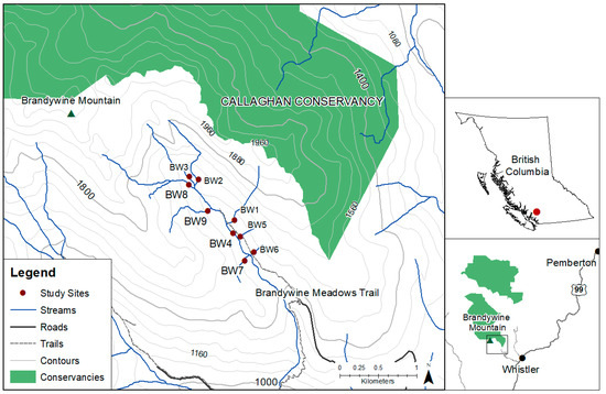
Figure 1.
Map of study site on Brandywine Mountain near Whistler, British Columbia. Solid circles represent nine survey sites, labeled BW1–BW9. Study sites were manually compiled based on longitude/latitude coordinates collected in the field. All other data layers were accessed through DataBC and compiled in ArcMap 10.7.1.
Brandywine Mountain is in the Dsb climate class (Köppen–Geiger Climate Classification), a continental subarctic climate with dry, warm summers [48]. The nearby ocean acts to moderate temperatures throughout the year, making temperature extremes rare in the area. Air coming off the water rises over the mountains and releases its precipitation as it climbs up the western flank of the mountain range, creating relatively drier conditions on the eastern side of the range, where the study site is located. The mean annual air temperature and precipitation of the site are 3.9 °C and 1350 mm, respectively. The majority of precipitation falls in the winter as snow (approximately 80%) and accumulates at high elevations where it melts over the summer months, feeding many small streams in the alpine meadows. BW4 is a second-order stream, while the remainder are first-order. These alpine streams drain from very shallow soils, meaning that they are very sensitive to the amount and timing of snowmelt.
2.2. Sampling
Nine streams were sampled within a single catchment, all flowing into Brandywine Creek, in the alpine meadows of Brandywine Mountain (Figure 1). Most streams had both step-pool and riffle-pool reach types. Streams were selected to represent a wide range of environmental conditions, mainly size (measured as width and depth), velocity indices and gradient. The nine streams maintained moderate flows (>0.6 m3/s) and low temperatures (6 to 14 °C) through the sampling period. No fish were present at any of the sites; the highest trophic level was generally occupied by chloroperlid and perlodid stoneflies.
In August 2019, five Surber samples (mesh size: 500 μm, sample area: 0.09 m2) were collected from each of the nine study streams. Sampling locations were selected within riffles and glides and spaced between 2 and 5 m apart depending on the length of the available channel and ranging from 15 to 25 m to represent the reach. Prior to collecting the Surber samples, measures of velocity and depth were collected at each sampling location. Three depth measures and five velocity measures were taken per sample and averaged to produce a single measure per sample. Velocity was measured with a flow meter at site BW2, but we had to use the float method at other sites [49] for all other streams. Following this, the Surber sampler was placed in the channel and substrate within the quadrat was disturbed to 10 cm depth over the course of one minute to dislodge and capture any benthic invertebrates present. Samples were placed into plastic jars and stored in 70% ethanol for identification in the lab. Benthic samples were sifted through multiple sieve mesh sizes for easier picking, and all animals ≥500 µm were picked and identified under a compound microscope. Identification was completed to the lowest taxonomic level practical using appropriate keys [50,51]. We also considered community composition based on Functional Feeding Groups (FFGs) to compare different trophic groupings.
While Surber samples were being collected, environmental variables were recorded for each stream. Spot measurements of pH, electrical conductivity, dissolved oxygen and temperature were taken using a YSI probe (YSI Model 556 MPS). Stream gradient was measured using a Suunto clinometer; gradient measures were taken over the length of the sampling reach. In addition, wetted width and bankfull width were measured at three evenly spaced points across the sampling reach. Water samples were collected from all 9 streams following the collection of benthic samples and immediately prior to leaving the study site. Water samples were frozen until they could be analyzed by the Analytical Chemical Research Laboratory in Victoria, BC (a branch of the BC Ministry of Environment and Climate Change). Analyses of water samples returned data on concentrations of chloride, sulphate, ammonium and dissolved organic carbon (DOC). However, analyses of concentrations of bromide, fluoride, nitrates, nitrites, phosphates and total suspended solids were below detection limits (<0.1 mg/L for bromide, fluoride, nitrates and nitrites; <0.5 mg/L for phosphates; <4 mg/L for total suspended solids).
2.3. Statistical Analyses
Data were analyzed in R 4.0.3 [52]. Assumptions of normality, linearity and equal variances were tested on the data prior to analyses and those that did not meet assumptions were transformed using the natural log (ln) or inverse of the response variable. Environmental variables were put through a correlation analysis using rcorr in the package ‘Hmsic’ and principal component analysis (PCA, prcomp in package ‘stats’) to assess the correlation structure and to determine which variables explained the greatest difference among the streams. Those variables with low correlation to other variables or that were shown to have the largest eigenvalues were chosen for regression analysis, i.e., slope, bankfull width and pH. We regressed mean taxon richness and mean percent composition of Ephemeroptera, Plecoptera and Trichoptera (EPT) taxa against the three selected environmental variables. The density for all samples were analyzed in an ANOVA to partition within-stream variation compared to between-stream variation.
Single species’ total abundances were regressed against the three selected environmental variables to explore any relationships found in the previous analyses. Only those taxa found in 7 or more of the surveyed streams were considered to be sufficiently present across the study area and were thus used for these analyses (see Table A3 for the full list of taxa examined). Each invertebrate taxon was assigned to functional feeding groups (FFGs) based on [50,51]. Four broad groups were classified: shredders, collectors, scrapers and predators. In cases where taxa fit into more than one FFG, values were split between groups by dividing abundance values by the number of FFGs assigned. From this information, community trophic structure measures were calculated for each stream: mean percent shredders, collectors, scrapers and predators.
Additional analyses consisted of beta diversity analysis and non-metric multidimensional scaling (NMDS). Invertebrate community data were analyzed for beta diversity using vegdist in the package ‘vegan’. The Bray–Curtis dissimilarity equation was used for this analysis, chosen due to its consideration of species abundances and its removal of double-zeros from the calculation. Two dimensional NMDS analyses were conducted using metaMDS in the package ‘vegan’ to compare community structure across the nine sites. Invertebrates that made up less than 0.5% of the total number of individuals across all samples were removed for this analysis. Two dimensions were selected as this showed the greatest decrease in stress values when plotted with results for higher numbers of dimensions. The Bray–Curtis dissimilarity measure was used to calculate values and data were autotransformed through a square root transformation. Ellipses were drawn around four invertebrate orders to provide a visual distinction between taxa within the ordination space. Environmental variables were fit into the ordination space using envfit from the package ‘vegan’ to determine which environmental variables were most strongly correlated with the calculated site values.
3. Results
3.1. Environmental Variables Analyses
Data for fourteen environmental variables were summarized for each stream, encompassing water quality and the physico-chemical components of these oligotrophic streams and catchment (Table 2). As noted in the Methods section, nutrient levels were below detection levels. Stream widths varied between 0.78 and 7.35 m, slope ranged from 1 to 31.5%, and pH varied between 6.74 and 9.2 (Table 2). Wetted width and bankfull width were highly correlated, so only bankfull width is shown. Temperatures at the time of sampling ranged from 6 to 14 °C. A correlation matrix for all environmental variables was created (Table 3). Measures of stream size were strongly positively correlated, e.g., catchment area and stream width (wetted width: p < 0.01, bankfull width: p < 0.01). Multiple measures of stream size and slope were strongly negatively correlated: slope and depth (p = 0.03), velocity and stream width (p = 0.01), and velocity and depth (p = 0.02). Conductivity and pH were positively correlated (p < 0.01), as was slope and DOC (p = 0.01). Environmental variables that were not correlated included temperature and elevation (p = 0.95), as well as sulphates and elevation (p = 0.94).
Table 2.
Environmental parameters representing water quality and stream flow and morphology indices for each of the nine streams included in the study. All nine streams are situated in one main catchment and range in elevation from 1410 to 1509 m. DOC = dissolved organic carbon.
Table 3.
p-values from Pearson’s correlation analysis of stream environmental variables collected across nine study sites. Values in bold font represents significant correlations and italicized values represent negative correlations.
Environmental variables were subsequently analyzed using principal component analysis (PCA; Figure 2). Initial PCA results showed the first axis being strongly differentiated by stream size and the second axis being differentiated by measures of water quality. Based on the results of the PCA and the correlation values we selected bankfull width, slope and pH as the most representative environmental variables (Table A1 and Table A2).
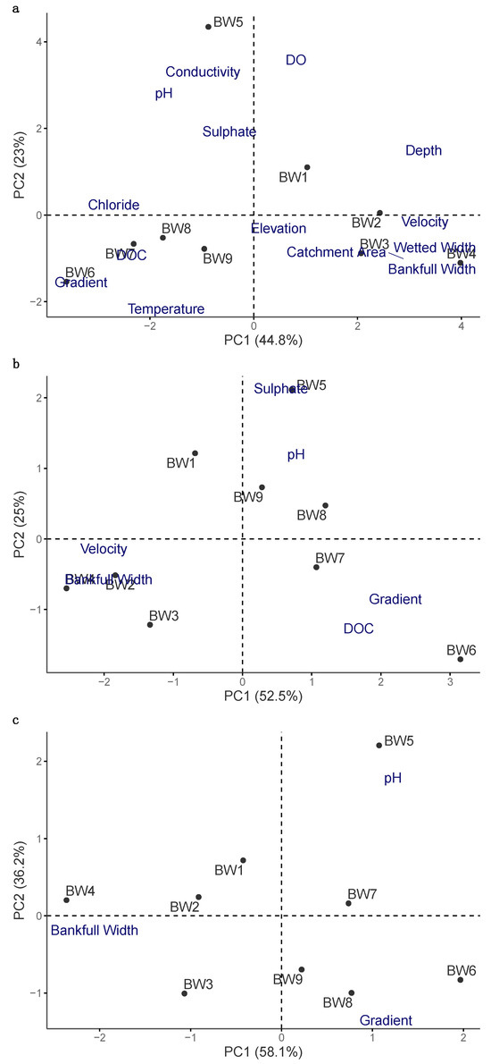
Figure 2.
Principal component analysis (PCA) results for environmental variables in nine streams in Brandywine Meadows; (a) PCA conducted for all environmental variables; (b) PCA conducted after removal of highly correlated variables or variables with low explanatory power; (c) PCA after removal of additional environmental variables, with bankfull width, gradient and pH remaining in the final analysis.
3.2. Community Analyses
In total, 10,393 invertebrates were identified and counted. The mean density of individuals across all streams was 2566 (SE ± 898, n = 9) individuals/m2 (Figure 3), while mean density per stream ranged from 596 to 7340 individuals/m2. Most of the nine streams exhibited small variation in density, with the exception of BW3. We used an ANOVA of all samples across all streams to partition the amount of between-stream variation relative to within-stream variation (n = 5 samples per stream). Variation between streams was 44% of the total variation (F8,36 = 3.58, p < 0.004). Density had no relationship with the three environmental variables examined (width: p = 0.64, R2 = 0.03, Figure 3; slope: p = 0.84, R2 = 0.01; pH: p = 0.86, R2 = 0.01).
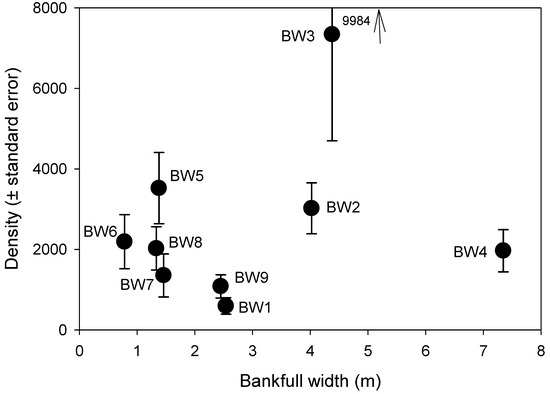
Figure 3.
Within-site variation (mean and standard error) of invertebrate density across nine streams in the study site, plotted by stream bankfull width (n = 5 samples per stream). Arrow at top indicates the end value of the error bar for BW3.
Of the identified invertebrates, most to the genus or subfamily level, 64 taxa were recorded, with 30 to 45 taxa per stream, with an average of 37 taxa (Table A3). Eight taxa were found in only one stream each, while seven were found in all nine streams. Of the total individuals sampled, 30.6% were Chironomidae, 25.2% were Ephemeroptera and 20.8% were Plecoptera (Table 4). After chironomids, Nemouridae was the next most abundant family at 12.7% of the total. Non-insect taxa (e.g., Oligochaeta, Acari, Nematoda), represented six of the taxa found and made up 17.5% of the total individuals sampled. The average percentage of EPT taxa was 51.8%, but with wide variation from 11.8 to 74.7% across the nine streams. Of all individuals sampled, 28.6% were collectors, 17.4% were scrapers, 17.8% were shredders and 14.3% were predators.
Table 4.
Mean values of measures of community structure and trophic feeding group composition measured across nine study sites (n = 5 samples per stream). EPT = Ephemeroptera, Plecoptera and Trichoptera.
Beta diversity (β) measures were calculated between communities in all streams (Bray–Curtis dissimilarity index; Table 5). There were many significant differences, with the highest beta diversity values (greatest dissimilarity) between streams BW2 and BW6 (β = 0.91), BW1 and BW3 (β = 0.87), and BW6 and BW9 (β = 0.85). The greatest similarity (lowest beta values) was found between streams BW5 and BW8 (β = 0.46), as well as BW2 and BW4 (β = 0.43).
Table 5.
Beta diversity (β) values across nine streams in Brandywine Meadows calculated using the Bray–Curtis dissimilarity equation. Higher values represent greater dissimilarity between streams than lower values. Values > 0.8 represent high beta diversity and are in bold font.
3.3. Regression Analyses
Simple linear regression revealed two significant relationships among the two community diversity indices and three key environmental variables we examined (with six comparisons, Bonferroni correction requires probabilities of p < 0.008). Mean percent EPT was positively related with stream width (p = 0.016, R2 = 0.59; Figure 4A) and negatively related with stream slope (p = 0.05, R2 = 0.45; Figure 4C). Mean percent EPT was not related to pH (p = 0.18, R2 = 0.24). Mean taxon richness showed a slightly positive trend with stream width, but no significant relationship was found (width: p = 0.21, R2 = 0.21). Additionally, mean taxon richness exhibited no relationship with slope (p = 0.65, R2 = 0.03) or pH (p = 0.35, R2 = 0.11). Note that we did not apply Bonferroni correction, but none of the relationships would be significant if we had.
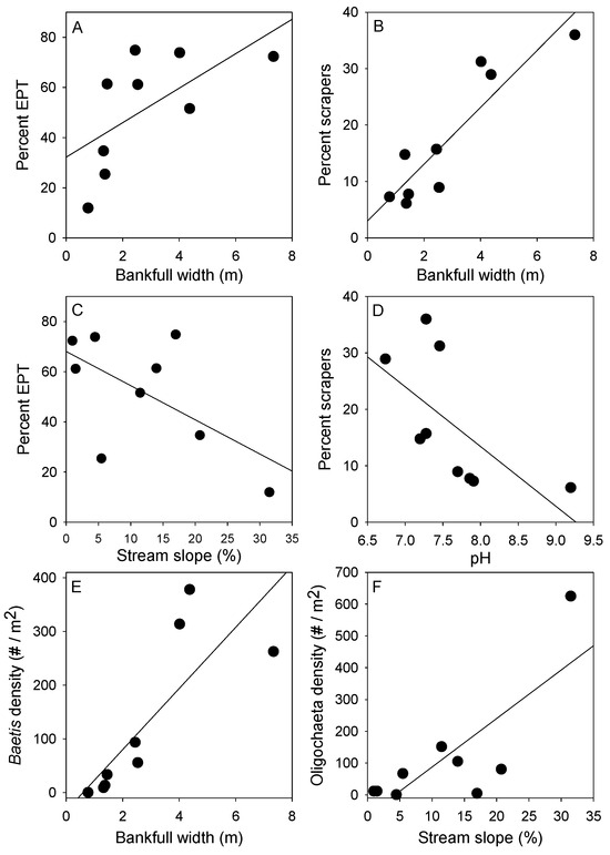
Figure 4.
Regression plots of the relationships between percent EPT taxa and other measures versus the three selected environmental parameters. These benthic communities were sampled from nine alpine streams in southwestern British Columbia. Points represent the mean value per stream for each of the nine streams. (A) Percent EPT versus Bankfull width; (B) Percent scrapers versus Bankfull width; (C) Percent EPT versus Stream slope; (D) Percent scrapers versus pH; (E) Baetis density versus Bankfull width; (F) Oligochaeta density versus Stream slope.
For percentages in each functional feeding group, three had significant relationships with environmental variables. Collector percentages were significantly negatively related to slope (p = 0.04, R2 = 0.48), and scraper percentages exhibited a positive significant relationship with stream width (p = 0.003, R2 = 0.73; Figure 4B) and a negative significant relationship with pH (p = 0.03, R2 = 0.51; Figure 4D). No other regressions of FFGs against environmental variables were significant.
To complement regression analyses of community-based indices, simple linear regressions were conducted on single taxa found in the majority (>7) of the study streams. Of the 20 taxa we examined, 5 exhibited significant relationships with stream environmental variables (note, multiple comparisons requires p < 0.0025). Baetis (Baetidae) abundances were significantly positively related to stream width (p = 0.023, R2 = 0.55; Figure 4E). The abundances of three non-insect taxa were significantly positively related to slope (Oligochaeta: p = 0.015, R2 = 0.59, Figure 4F; Nematoda: p = 0.019, R2 = 0.57; Acari: p = 0.013, R2 = 0.61). Turbellaria abundances were significantly positively related to pH (p = 0.04, R2 = 0.47).
3.4. Non-Metric Multidimensional Scaling Analysis
For two-dimensional NMDS of abundance data across communities (k = 2), the stress value was 0.18 and the non-metric R2 value was 0.998. Environmental variables found to be significantly or near-significantly (p ≤ 0.1) related to NMDS values for invertebrate community data were velocity (p = 0.004), DOC (p = 0.063), chloride (p = 0.096), bankfull width (p = 0.098) and gradient (p = 0.1). The first NMDS axis was defined by velocity, width and DOC, while the second axis was defined by slope, chloride concentration, velocity and width. The communities of the different streams were aligned by stream based on stream size (generally small to the negative, large to the positive), velocity (slow to the negative, fast positive) and DOC (high to negative, low positive) (Figure 5).
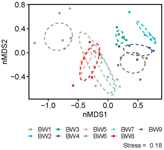
Figure 5.
NMDS plots of the communities from nine alpine, non-glacial streams in southwest British Columbia. Ellipses represent the 95% confidence intervals around the five samples per stream.
4. Discussion
Stream invertebrates are an important part of the ecosystem structure and contribute substantially to the functioning of streams. Nine nearby streams representing a small gradient of sizes, slopes and water chemistry, all within a single alpine meadow, exhibited large differences in abundances of certain taxa and the communities they were part of. In these ultraoligotrophic streams, there were significant differences in beta diversity between the nine streams, even over such a small area and gradient of environmental features. The mechanisms leading to large differences in a small area are not clear, although the evidence points to strong environmental filters, as dispersal limitation is unlikely to account for the observed patterns. We tested for relationships between environmental features and abundances or percentage of certain groups, and there were some clear patterns, although we point out that with the multiple comparisons made, that none would strictly be considered significant. Given that, in the context of this work, we were looking for patterns to generate future hypotheses, and with the descriptive nature of this work, we relaxed this strict criterion.
There were some apparent relations between densities of certain taxa or feeding groups with the key environmental factors, noting the issue of multiple comparisons. The mayflies Baetis, Cinygmula and Epeorus all had positive relations, but not significant, with current velocity, consistent with what is known of their biology [53]. There was considerable variation in overall density between streams, given their proximity, all within 1.2 km of each other. Stream BW3 had a much higher density and taxonomic richness of invertebrates than the other streams, while the only distinctive feature of this stream was that it had a slightly lower pH than the others.
4.1. Water Quality
The relatively high DOC concentrations in BW6 and BW7 were unexpected in this alpine meadow, but they may be associated with small wetland areas upstream. From the correlation analysis, we found a positive correlation between slope and DOC concentration, in contrast to other studies [54,55]. Glacial streams typically have very low DOC, as there are few sources associated with glacier melt. The DOC concentrations in these streams were comparable to what is found in small, forest streams in the region [56]. However, despite relatively high DOC concentrations, this was not reflected in higher densities of invertebrates in those two streams, and we did not have any measures of biofilm biomass.
We found a relatively large gradient in pH across these nine streams, from 6.7 to 9.2. The primary bedrock in this site is quartz diorite intrusives, but other geologic forms occur in this volcanic area [57]. Local surficial and bedrock features in complex geologic areas could account for such variation in pH, and this was another aspect contributing to the environmental heterogeneity across streams within this alpine meadow.
4.2. Macroinvertebrates
Taxonomic diversity was much higher (30 to 45 taxa per stream) than in many glacial streams and similar to other non-glacial streams. However, notably we found no Diamesa spp. in our streams, which is a chironomid genus that is typically the most common taxon in glacially dominated alpine streams [26,36,41]. Diamesa are capable of tolerating high water temperatures [28]. However, in studies looking at the effects of glaciers on invertebrate communities, Diamesa tend to disappear as temperatures increase, likely due to being outcompeted by orthoclads [26]. Diamesa sp. is known from sites in the Rocky Mountains, over 1000 km east of our sites [58]. However, lack of broader surveys in these Coast Mountain streams means that we do not know if Diamesa spp. are present or absent in the region.
Bryophytes and Nostoc colonies provide important habitat in streams, particularly those lacking woody material and detrital accumulations. In particular, larvae of the chironomid Cricotopus use colonies of the cyanobacteria Nostoc as a habitat within which they burrow [59]. These species were quite common in some streams, such as BW5, where it was 100 times more abundant than in any of the other eight streams. Cricotopus was entirely lacking in some streams, such as BW7, 8 and 9. Why one stream had such a high standing stock of Nostoc, and by extension Cricotopus, is not obvious. However, BW5 also had very high conductivity and pH compared to the other eight streams, perhaps representing some volcanic geological inclusions in this coastal mountain range [57].
Bryophytes provide important habitat to many invertebrates, in addition to accumulating fine particulate organic matter [35,60,61]. Most of our study streams had abundant growths of mosses. We did not quantify moss cover, but as with Nostoc, some streams had greater coverage of mosses than in other streams, again emphasizing the differences in stream communities over a small spatial extent.
There were considerable differences in the trophic groupings across the nine streams. Although the shredder feeding group made up an average of 18.7% of the total numbers, there was little to no coarse detrital material in these alpine streams. Many species of nemourids and capniids (Plecoptera) are capable of feeding on biofilms, whether these are the surfaces of leaves, wood or rock [36]. Some species in these two families are found in glacial and non-glacial alpine streams, such as Lednia spp. and Zapada spp. [33,34].
Communities of the nine streams were substantially different, as seen in the NMDS, over a relatively small gradient of stream sizes and geomorphology. This variation was seen in the taxonomic and trophic structure of the streams. The streams that differed the most in the NMDS state space along NMDS axis 1 were distinguishable based on their size (generally small to the negative, large to the positive), velocity (slow to the negative, fast positive) and DOC (high to negative, low positive). Other studies of macroinvertebrates communities in temperate and boreal streams have generally found stream size is a major variable in determining community structure [62,63]. Likewise, invertebrate abundance varies with stream gradient and velocity [63]. These gradients may be quantitatively small, but it appears they have large influences on stream communities.
4.3. Beta Diversity
We found high β diversity values between many streams, indicating large compositional differences in a small area. High β diversity can be due to dispersal limits, productivity differences, or environmental heterogeneity, the latter of which appears to be the case in our study. In studies of glacially influenced streams, estimates of β diversity were over 0.8, and as high as 0.85, so high values seem to be the norm in high-elevation streams [64,65]. Likewise, high β diversity was found among headwater mountain streams in California, consistent with environmental filtering and isolation [66]. Our streams had β diversity values similar to or higher than any of the five watersheds studied in California, where their highest value was 7.0 [66]. Those authors also found an inverse relationship between community size (richness) and β diversity. One of the contributors to high β diversity can be the presence of non-insect invertebrates with lower dispersal capacity than aquatic insects, but the differences were only very slightly accounted for by these less mobile taxa. Our results are consistent with environmental filtering (species sorting) due to habitat heterogeneity on a small spatial scale, i.e., a single alpine meadow.
High β diversity was found between streams within drainages in a global analysis, but variables available explained less variation than expected, suggesting disturbance might be another cause [67]. Other studies of invertebrates in temperate forest streams have found large differences across streams and high β diversity values, although often across much larger spatial scales than our study [64,67]. Streams in a small area may offer more environmental heterogeneity between them than often considered.
We found that some species (eight) were found in only one of our nine streams, indicating a high potential for endemism. Other studies have noted the high degree of endemism of macroinvertebrate taxa in alpine streams [66,68]. This relatively unexplored component of biodiversity suggests that more needs to be known about these poorly studied communities if agencies are to manage such ecosystems in the face of climate change and other land uses.
5. Conclusions
As the frequency and magnitude of droughts due to climate change and other anthropogenic land-use modifications are predicted to increase in mountain areas [35], studies of the biological characteristics of these sentinel ecosystems could be useful for monitoring. Too little is known about alpine streams in Canada, and emphasis on fish-bearing streams leads to little attention being given to these source streams. Non-glacial, alpine streams with their benthic species and functional diversity play a key role in the riverine ecological network [11,66].
The large differences in communities as reflected by high beta diversity values in a small area (<1.2 km long) highlight the potential for endemism and unique communities in these alpine, non-glacial stream ecosystems. The mechanisms responsible for local specialization are not clear, but the associations we found between communities and the physico-chemical environments suggest strong environmental filtering of the community composition.
Author Contributions
Conceptualization, S.S. and J.S.R.; methodology, S.S. and J.S.R.; validation, S.S., J.S.R. and Y.S.; formal analysis, Y.S. and J.S.R.; investigation, S.S.; resources, J.S.R.; data curation, J.S.R.; writing—original draft preparation, S.S. and J.S.R.; writing—review and editing, S.S., Y.S. and J.S.R.; visualization, S.S., J.S.R. and Y.S.; supervision, J.S.R.; project administration, J.S.R.; funding acquisition, J.S.R. All authors have read and agreed to the published version of the manuscript.
Funding
This research was funded by the Natural Sciences and Engineering Research Council (Canada), grant number RGPIN-2018-03838.
Institutional Review Board Statement
Ethical review and approval were waived for this study due to use of invertebrates.
Informed Consent Statement
Not applicable.
Data Availability Statement
The data are available by request from the corresponding author due to ongoing use in related studies.
Conflicts of Interest
The authors declare no conflicts of interest.
Appendix A
Table A1.
Principal component loading scores based on PCA run on three environmental variables (Figure 2c), measured across nine study streams.
Table A1.
Principal component loading scores based on PCA run on three environmental variables (Figure 2c), measured across nine study streams.
| PC1 | PC2 | PC3 | |
|---|---|---|---|
| Gradient | 0.5575 | −0.6099 | −0.5632 |
| Bankfull Width | −0.7258 | −0.0288 | −0.6873 |
| pH | 0.4030 | 0.7919 | −0.4588 |
Table A2.
Site scores based on principal component analysis run on three environmental variables (bankfull width, gradient and pH; Figure 2c) measured in nine study streams.
Table A2.
Site scores based on principal component analysis run on three environmental variables (bankfull width, gradient and pH; Figure 2c) measured in nine study streams.
| PC1 | PC2 | PC3 | |
|---|---|---|---|
| BW1 | −0.42 | 0.72 | 0.64 |
| BW2 | −0.91 | 0.24 | 0.14 |
| BW3 | −1.07 | −1.01 | 0.11 |
| BW4 | −2.36 | 0.20 | −0.64 |
| BW5 | 1.07 | 2.20 | −0.20 |
| BW6 | 1.97 | -0.83 | −0.60 |
| BW7 | 0.74 | 0.16 | 0.19 |
| BW8 | 0.77 | −1.00 | 0.29 |
| BW9 | 0.22 | −0.70 | 0.08 |
Table A3.
Full list of taxa found in the nine study streams and their total number, number of streams each taxon were found in order, family and FFG (functional feeding group). A total of 10,393 invertebrates were identified in this study from 64 different taxa. Some taxa, including pupae, only identified to morphospecies, and not separated in the table. FFG abbreviations: SC = scraper, CG = collector–gatherer, CF = collector–filterer (grouped with collector–gatherers for analyses), SH = shredders, PR = predators.
| Taxa | Total Individuals | Number of Streams | Order/Family | FFG |
|---|---|---|---|---|
| Ameletus | 70 | 9 | Ephemeroptera/Ameletidae | SC/CG |
| Baetis | 521 | 8 | Ephemeroptera/Baetidae | CG |
| Drunella doddsi | 35 | 4 | Ephemeroptera/Ephemerellidae | SC |
| Seratella | 1 | 1 | Ephemeroptera/Ephemerellidae | CG |
| Eurylophella | 103 | 6 | Ephemeroptera/Ephemerellidae | CG |
| Rhithrogena | 305 | 7 | Ephemeroptera/Heptageniidae | SC |
| Cinygmula | 649 | 9 | Ephemeroptera/Heptageniidae | SC |
| Epeorus | 145 | 7 | Ephemeroptera/Heptageniidae | SC |
| Paraleptophlebia | 790 | 8 | Ephemeroptera/Leptophlebiidae | CG |
| Zapada haysi | 3 | 3 | Plecoptera/Nemouridae | SH |
| Zapada frigida | 860 | 9 | Plecoptera/Nemouridae | SH |
| Malenka | 4 | 4 | Plecoptera/Nemouridae | SH |
| Visoka | 14 | 4 | Plecoptera/Nemouridae | SH |
| Podmosta | 450 | 6 | Plecoptera/Nemouridae | SH |
| Capnia | 37 | 8 | Plecoptera/Capniidae | SH |
| Kathroperla | 26 | 6 | Plecoptera/Chloroperlidae | CG |
| Other Chloroperlidae | 505 | 9 | Plecoptera/Chloroperlidae | PR |
| Setvena | 4 | 2 | Plecoptera/Perlodidae | PR |
| Megarcys | 2 | 2 | Plecoptera/Perlodidae | PR |
| Perlodid 1 | 109 | 9 | Plecoptera/Perlodidae | PR |
| Taeniopterygidae | 160 | 3 | Plecoptera/Taeniopterygidae | SH |
| Moselia | 4 | 1 | Plecoptera/Leuctridae | SH |
| Perlomyia | 26 | 5 | Plecoptera/Leuctridae | SH |
| Agapetus | 4 | 2 | Trichoptera/Glossosomatidae | SC |
| Parapsyche | 7 | 4 | Trichoptera/Hydropsychidae | CF |
| Arctopsyche | 2 | 2 | Trichoptera/Hydropsychidae | CF |
| Rhyacophila | 100 | 8 | Trichoptera/Rhyacophilidae | PR/CG |
| Polycentropus | 3 | 3 | Trichoptera/Polycentropodidae | PR/CF |
| Lepidostomatidae | 3 | 3 | Trichoptera/Lepidostomatidae | SH |
| Micrasema | 6 | 3 | Trichoptera/Brachycentridae | SH/CG |
| Frenesia | 1 | 1 | Trichoptera/Limnephilidae | SH |
| Allomyia | 2 | 1 | Trichoptera/Limnephilidae | SH/SC |
| Ecclisomyia | 2 | 1 | Trichoptera/Limnephilidae | CG |
| Phanocelia | 3 | 2 | Trichoptera/Limnephilidae | SH |
| Limnephilidae spp. | 6 | 4 | Trichoptera/Limnephilidae | SH |
| Neothremma | 6 | 3 | Trichoptera/Uenoidae | SC/CG |
| Corydalidae | 1 | 1 | Megaloptera/Corydalidae | PR |
| Tanytarsini | 54 | 8 | Diptera/Chironomidae | CF/CG |
| Tanypodinae | 88 | 9 | Diptera/Chironomidae | PR |
| Brillia retifinis | 369 | 9 | Diptera/Chironomidae | SH/CG |
| Corynoneura | 269 | 9 | Diptera/Chironomidae | CG |
| Cricotopus | 466 | 5 | Diptera/Chironomidae | SH/CG |
| Other Orthocladiinae | 1650 | 9 | Diptera/Chironomidae | CG/SC |
| Chironomid 1 | 3 | 2 | Diptera/Chironomidae | CG/SC |
| Ceratopogonidae | 156 | 8 | Diptera/Chironomidae | PR |
| Simuliidae | 268 | 5 | Diptera | CF |
| Chelifera | 54 | 7 | Diptera/Empididae | -- |
| Oreogeton | 154 | 7 | Diptera/Empididae | -- |
| Tipulidae | 1 | 1 | ||
| Dytiscidae | 1 | 1 | PR | |
| Colembolla | 42 | 9 | ||
| Ostracoda | 165 | 5 | -- | -- |
| Copepoda | 41 | 4 | -- | -- |
| Oligochaeta | 474 | 8 | -- | -- |
| Turbellaria | 124 | 7 | -- | -- |
| Nematoda | 310 | 9 | -- | -- |
| Acari | 454 | 9 | -- | -- |
References
- IPCC. Climate Change: Synthesis Report. In Contribution of Working Groups I, II and III to the Fifth Assessment Report of the Intergovernmental Panel on Climate Change; Pachauri, R.K., Meyer, L., Eds.; IPCC: Geneva, Switzerland, 2014. [Google Scholar]
- Salathé, E.P.; Steed, R.; Mass, C.F.; Zahn, P.H. A high-resolution climate model for the U.S. Pacific northwest: Mesoscale feedbacks and local responses to climate change. J. Clim. 2008, 21, 5708–5726. [Google Scholar] [CrossRef]
- Clarke, G.K.C.; Jarosch, A.H.; Anslow, F.S.; Radić, V.; Menounos, B. Projected deglaciation of western Canada in the twenty-first century. Nat. GeoSci. 2015, 8, 372–377. [Google Scholar] [CrossRef]
- Pederson, G.T.; Graumlich, L.J.; Fagre, D.B.; Kipfer, T.; Muhlfeld, C.C. A century of climate and ecosystem change in Western Montana: What do temperature trends portend? Clim. Change 2010, 98, 133–154. [Google Scholar] [CrossRef]
- McCullough, I.M.; Davis, F.W.; Dingman, J.R.; Flint, L.E.; Serra-Diaz, J.M.; Syphard, A.D.; Moritz, M.A.; Hannah, L.; Franklin, J. High and dry: High elevations disproportionately exposed to regional climate change in Mediterranean-climate landscapes. Landsc. Ecol. 2016, 31, 1063–1075. [Google Scholar] [CrossRef]
- Beniston, M.; Farinotti, D.; Stoffel, M.; Andreassen, L.M.; Coppola, E.; Eckert, N.; Fantini, A.; Giacona, F.; Hauck, C.; Huss, M.; et al. The European mountain cryosphere: A review of its current state, trends, and future challenges. Cryosphere 2018, 12, 759–794. [Google Scholar] [CrossRef]
- Barnett, T.P.; Adam, P.; Lettenmaier, J.C. Potential impacts of a warming climate on water availability in snow-dominated regions. Nature 2005, 438, 303–309. [Google Scholar] [CrossRef] [PubMed]
- von Fumetti, S.; Bieri-Wigger, F.; Nagel, P. Temperature variability and its influence on macroinvertebrate assemblages of alpine springs. Ecohydrology 2017, 10, e1878. [Google Scholar] [CrossRef]
- Brown, L.E.; Hannah, D.M.; Milner, A.M. Hydroclimatological influences on water column and streambed thermal dynamics in an alpine river system. J. Hydrol. 2006, 325, 1–20. [Google Scholar] [CrossRef]
- Walters, A.W.; Post, D.M. How low can you go? Impacts of a low-flow disturbance on aquatic insect communities. Ecol. Applic. 2011, 21, 163–174. [Google Scholar] [CrossRef]
- Piano, E.; Doretto, A.; Mammola, S.; Falasco, E.; Fenoglio, S.; Bona, F. Taxonomic and functional homogenisation of macroinvertebrate communities in recently intermittent Alpine watercourses. Freshwat. Biol. 2020, 65, 2096–2107. [Google Scholar] [CrossRef]
- Füreder, L. High alpine streams: Cold habitats for insect larvae. In Cold-Adapted Organisms; Margesin, R., Schinner, F., Eds.; Springer: Berlin/Heidelberg, Germany, 1999; pp. 181–196. [Google Scholar]
- Brown, L.E.; Hannah, D.M.; Milner, A.M. Alpine stream habitat classification: An alternative approach incorporating the role of dynamic water source contributions. Arct. Antarct. Alp. Res. 2003, 35, 313–322. [Google Scholar] [CrossRef]
- Ward, J.V. Ecology of alpine streams. Freshwat. Biol. 1994, 32, 277–294. [Google Scholar] [CrossRef]
- Khamis, K.; Brown, L.E.; Hannah, D.M.; Milner, A.M. Glacier–groundwater stress gradients control alpine river biodiversity. Ecohydrology 2016, 9, 1263–1275. [Google Scholar] [CrossRef]
- Milner, A.M.; Gloyne-Phillips, I.T. The role of riparian vegetation and woody debris in the development of macroinvertebrate assemblages in streams. River Res. Appl. 2005, 21, 403–420. [Google Scholar] [CrossRef]
- Cowie, N.M.; Moore, R.D.; Hassan, M.A. Effects of glacial retreat on proglacial streams and riparian zones in the Coast and North Cascade Mountains. Earth Surf. Process. Landf. 2014, 39, 351–365. [Google Scholar] [CrossRef]
- Milner, A.M.; Petts, G.E. Glacial rivers: Physical habitat and ecology. Freshwat. Biol. 1994, 32, 295–307. [Google Scholar] [CrossRef]
- Rott, E.; Cantonati, M.; Füreder, L.; Pfister, P. Benthic algae in high altitude streams of the Alps—A neglected component of the aquatic biota. Hydrobiologia 2006, 562, 195–216. [Google Scholar] [CrossRef]
- Uehlinger, U.; Robinson, C.T.; Hieber, M.; Zah, R. The physico-chemical habitat template for periphyton in alpine glacial streams under a changing climate. Hydrobiologia 2010, 657, 107–121. [Google Scholar] [CrossRef]
- Clitherow, L.R.; Carrivick, J.L.; Brown, L.E. Food web structure in a harsh glacier-fed river. PLoS ONE 2013, 8, e60899. [Google Scholar] [CrossRef]
- Brown, L.E.; Milner, A.M.; and Hannah, D.M. Groundwater influence on alpine stream ecosystems. Freshwat. Biol. 2007, 52, 878–890. [Google Scholar] [CrossRef]
- Brown, L.E.; Céréghino, R.; Compin, A. Endemic freshwater invertebrates from southern France: Diversity, distribution and conservation implications. Biol. Conserv. 2009, 142, 2613–2619. [Google Scholar] [CrossRef]
- Thompson, C.; David, E.; Freestone, M.; Robinson, C.T. Ecological patterns along two alpine glacial streams in the Fitzpatrick Wilderness, Wind River Range, USA. West. N. Am. Nat. 2013, 73, 137–147. [Google Scholar] [CrossRef]
- Alther, R.; Thompson, C.; Lods-Crozet, B.; Robinson, C.T. Macroinvertebrate diversity and rarity in non-glacial Alpine streams. Aquat. Sci. 2019, 81, 1–14. [Google Scholar] [CrossRef]
- Milner, A.M.; Brittain, J.E.; Castella, E.; Petts, G.E. Trends of macroinvertebrate community structure in glacier-fed rivers in relation to environmental conditions: A synthesis. Freshwat. Biol. 2001, 46, 1833–1847. [Google Scholar] [CrossRef]
- Gao, W.; Gao, S.; Li, Z.; Lu, X.X.; Zhang, M.; Wang, S. Suspended sediment and total dissolved solid yield patterns at the headwaters of Urumqi River, northwestern China: A comparison between glacial and non-glacial catchments. Hydrol. Process. 2014, 28, 5034–5047. [Google Scholar] [CrossRef]
- Lencioni, V.; Barcelo, D. Glacial influence and stream macroinvertebrate biodiversity under climate change: Lessons from the Southern Alps. Sci. Total Environ. 2017, 622, 563–575. [Google Scholar] [CrossRef] [PubMed]
- Füreder, L.; Niedrist, G.H. Glacial stream ecology: Structural and functional assets. Water 2020, 12, 376. [Google Scholar] [CrossRef]
- Jacobsen, D.; Cauvy-Fraunie, S.; Andino, P.; Espinosa, R.; Cueva, D.; Dangles, O. Runoff and the longitudinal distribution of macroinvertebrates in a glacier-fed stream: Implications for the effects of global warming. Freshwat. Biol. 2014, 59, 2038–2050. [Google Scholar] [CrossRef]
- Cauvy-Fraunié, S.; Espinosa, R.; Andino, P.; Jacobsen, D.; Dangles, O. Invertebrate metacommunity structure and dynamics in an Andean glacial stream network facing climate change. PLoS ONE 2015, 10, e0136793. [Google Scholar] [CrossRef]
- Zimmer, A.; Meneses, R.I.; Rabatel, A.; Soruco, A.; Dangles, O.; Anthelme, F. Time lag between glacial retreat and upward migration alters tropical alpine communities. Perspect. Pl. Ecol. Evol. Syst. 2018, 30, 89–102. [Google Scholar] [CrossRef]
- Giersch, J.J.; Hotaling, S.; Kovach, R.P.; Jones, L.A.; Muhlfeld, C.C. Climate-induced glacier and snow loss imperils alpine stream insects. Glob. Change Biol. 2017, 23, 2577–2589. [Google Scholar] [CrossRef]
- Hotaling, S.; Shah, A.A.; McGowan, K.L.; Tronstad, L.M.; Giersch, J.J.; Finn, D.S.; Woods, H.A.; Dillon, M.E.; Kelley, J.L. Mountain stoneflies may tolerate warming streams: Evidence from organismal physiology and gene expression. Glob. Change Biol. 2020, 26, 5524–5538. [Google Scholar] [CrossRef]
- Brighenti, S.; Tolotti, M.; Bertoldi, W.; Wharton, G.; Bruno, M.C. Rock glaciers and paraglacial features influence stream invertebrates in a deglaciating Alpine area. Freshwat. Biol. 2021, 66, 535–548. [Google Scholar] [CrossRef]
- Niedrist, G.H.; Füreder, L. Towards a definition of environmental niches in alpine streams by employing chironomid species preferences. Hydrobiologia 2016, 781, 143–160. [Google Scholar] [CrossRef]
- Sertić Perić, M.; Nielsen, J.M.; Schubert, C.J.; Robinson, C.T. Does rapid glacial recession affect feeding habits of alpine stream insects? Freshwat. Biol. 2021, 66, 114–129. [Google Scholar] [CrossRef]
- Niedrist, G.H.; Füreder, L. Real-time warming of Alpine streams: (re)defining invertebrates’ temperature preferences. River Res. Appl. 2021, 37, 283–293. [Google Scholar] [CrossRef]
- Llg, C.; Castella, E. Patterns of macroinvertebrate traits along three glacial stream continuums. Freshwat. Biol. 2006, 51, 840–853. [Google Scholar]
- Lencioni, V.; Franceschini, A.; Paoli, F.; Debiasi, D. Structural and functional changes in the macroinvertebrate community in Alpine stream networks fed by shrinking glaciers. Fundam. Appl. Limnol. 2021, 194, 237–258. [Google Scholar] [CrossRef]
- Chaves, M.L.; Rieradevall, M.; Chainho, P.; Costa, J.L.; Costa, M.J.; Prat, N. Macroinvertebrate communities of non-glacial high altitude intermittent streams. Freshwat. Biol. 2008, 53, 55–76. [Google Scholar] [CrossRef]
- di Cugno, N.; Robinson, C.T. Trophic structure of macroinvertebrates in alpine non-glacial streams. Fundam. Appl. Limnol. 2017, 190, 319–330. [Google Scholar] [CrossRef]
- Fenoglio, S.; Bo, T.; Cammarata, M.; López-Rodríguez, M.J.; Tierno De Figueroa, J.M. Seasonal variation of allochthonous and autochthonous energy inputs in an Alpine stream. J. Limnol. 2015, 74, 272–277. [Google Scholar] [CrossRef]
- Doretto, A.; Bona, F.; Falasco, E.; Morandini, D.; Piano, E.; Fenoglio, S. Stay with the flow: How macroinvertebrate communities recover during the rewetting phase in Alpine streams affected by an exceptional drought. River Res. Appl. 2019, 36, 91–101. [Google Scholar] [CrossRef]
- Leppi, J.C.; DeLuca, T.H.; Harrar, S.W.; Running, S.W. Impacts of climate change on August stream discharge in the Central-Rocky Mountains. Clim. Change 2012, 112, 997–1014. [Google Scholar] [CrossRef]
- Füreder, L.; Vacha, C.; Amprosi, K.; Bühler, S.; Hansen, C.M.E.; Moritz, C. Reference conditions of alpine streams: Phyisical habitat and ecology. Water Air Soil Pollut. 2002, 2, 275–294. [Google Scholar] [CrossRef]
- Huss, M.; Bookhagen, B.; Huggel, C.; Jacobsen, D.; Bradley, R.S.; Clague, J.J.; Vuille, M.; Buytaert, W.; Cayan, D.R.; Greenwood, G.; et al. Toward mountains without permanent snow and ice. Earth’s Future 2017, 5, 418–435. [Google Scholar] [CrossRef]
- Kottek, M.; Grieser, J.; Beck, C.; Rudolf, B.; Rubel, F. World map of the Köppen-Geiger climate classification updated. Meteorol. Z. 2006, 5, 259–263. [Google Scholar] [CrossRef] [PubMed]
- Gore, J.A.; Banning, J. Discharge Measurements and Streamflow Analysis. In Methods in Stream Ecology, 3rd ed.; Hauer, F.R., Lamberti, G.A., Eds.; Academic Press: Cambridge, MA, USA, 2017; Volume 1, pp. 49–70. [Google Scholar]
- Merritt, R.W.; Cummins, K.W.; Berg, M.B. (Eds.) An Introduction to the Aquatic Insects of North America, 5th ed.; Kendall-Hunt Publishing Company: Dubuque, IA, USA, 2019. [Google Scholar]
- Thorp, A.H.; Covich, A.P. (Eds.) Ecology and Classification of North American Freshwater Invertebrates, 3rd ed.; Elsevier: Amsterdam, The Netherlands, 2009. [Google Scholar]
- Team, R.C. R: A Language and Environment for Statistical Computing; R Foundation for Statistical Computing: Vienna, Austria, 2021. [Google Scholar]
- Wellnitz, T. How do stream grazers partition their benthic habitat? Hydrobiologia 2015, 760, 197–204. [Google Scholar] [CrossRef]
- Harms, T.K.; Edmonds, J.W.; Genet, H.; Creed, I.F.; Aldred, D.; Balser, A.; Jones, J.B. Catchment influence on nitrate and dissolved organic matter in Alaskan streams across a latitudinal gradient. J. Geophys. Res. Biogeosci. 2016, 121, 350–369. [Google Scholar] [CrossRef]
- Musolffa, A.; Fleckenstein, J.H.; Opitz, M.; Büttner, O.; Kumar, R.; Tittel, J. Spatio-temporal controls of dissolved organic carbon stream water concentrations. J. Hydrol. 2018, 566, 205–215. [Google Scholar] [CrossRef]
- Kiffney, P.M.; Richardson, J.S.; Feller, M.C. Fluvial and epilithic organic matter dynamics in headwater streams of southwestern British Columbia, Canada. Arch. Hydrobiol. 2000, 149, 109–129. [Google Scholar] [CrossRef]
- Cui, Y.; Miller, D.; Schiarizza, P.; Diakow, L.J. British Columbia digital geology. In British Columbia Ministry of Energy, Mines and Petroleum Resources, British Columbia Geological Survey Open File 2017-8; British Columbia Geological Survey (BCGS): Victoria, BC, Canada, 2017; pp. 1–9. [Google Scholar]
- Muhlfeld, C.C.; Cline, T.J.; Joseph Giersch, J.J.; Peitzsch, E.; Florentine, C.; Jacobsen, D.; Hotaling, S. Specialized meltwater biodiversity persists despite widespread deglaciation. Proc. Nat. Acad. Sci. USA 2020, 117, 12208–12214. [Google Scholar] [CrossRef]
- Dodds, W.K.; Marra, J.L. Behaviors of the midge, Cricotopus (Diptera: Chironomidae) related to mutualism with Nostoc parmelioides (Cyanobacteria). Aquat. Insects 1989, 4, 201–208. [Google Scholar] [CrossRef]
- Muotka, T.; Syrjänen, J. Changes in habitat structure, benthic invertebrate diversity, trout populations and ecosystem processes in restored forest streams: A boreal perspective. Freshwat. Biol. 2007, 52, 724–737. [Google Scholar] [CrossRef]
- Fritz, K.M.; Glime, J.M.; Hribljan, J.; Greenwood, J.L. Can bryophytes be used to characterize hydrologic permanence in forested headwater streams? Ecol. Indicat. 2009, 9, 681–692. [Google Scholar] [CrossRef]
- Malmqvist, B.; Hoffsten, P.-O. Macroinvertebrate taxonomic richness, community structure and nestedness in Swedish streams. Arch. Hydrobiol. 2000, 150, 29–54. [Google Scholar] [CrossRef]
- Danehy, R.J.; Chan, S.S.; Lester, G.T.; Langshaw, R.B.; Turner, T.R. Periphyton and macroinvertebrate assemblage structure in headwaters bordered by mature, thinned, and clearcut Douglas-fir stands. For. Sci. 2007, 53, 294–307. [Google Scholar] [CrossRef]
- Brown, L.E.; Hannah, D.M.; Milner, A.M. Vulnerability of alpine stream biodiversity to shrinking glaciers and snowpacks. Glob. Change Biol. 2007, 13, 958–966. [Google Scholar] [CrossRef]
- Finn, D.S.; Khamis, K.; Milner, A.M. Loss of small glaciers will diminish beta diversity in Pyrenean streams at two levels of biological organization. Glob. Ecol. Biogeogr. 2013, 22, 40–51. [Google Scholar] [CrossRef]
- Green, M.D.; Anderson, K.E.; Herbst, D.B.; Spasojevic, M.J. Rethinking biodiversity patterns and processes in stream ecosystems. Ecol. Monogr. 2022, 92, e1520. [Google Scholar] [CrossRef]
- Heino, J.; Melo, A.S.; Bini, L.M.; Altermatt, F.; Al-Shami, S.A.; Angeler, D.G.; Bonada, M.; Brand, C.; Callisto, M.; Cottenie, K.; et al. A comparative analysis reveals weak relationships between ecological factors and beta diversity of stream insect metacommunities at two spatial levels. Ecol. Evol. 2015, 5, 1235–1248. [Google Scholar] [CrossRef]
- Bonacina, L.; Eme, E.; Fornaroli, R.; Lamouroux, N.; Cauvy-Fraunié, S. Spatiotemporal patterns of macroinvertebrate assemblages across mountain streams with contrasting thermal regimes. Freshwat. Sci. 2023, 42, 392–408. [Google Scholar] [CrossRef]


Disclaimer/Publisher’s Note: The statements, opinions and data contained in all publications are solely those of the individual author(s) and contributor(s) and not of MDPI and/or the editor(s). MDPI and/or the editor(s) disclaim responsibility for any injury to people or property resulting from any ideas, methods, instructions or products referred to in the content. |
© 2025 by the authors. Licensee MDPI, Basel, Switzerland. This article is an open access article distributed under the terms and conditions of the Creative Commons Attribution (CC BY) license (https://creativecommons.org/licenses/by/4.0/).