Numerical Simulation of Hyperbolic Problems with Interface Discontinuities via Multi-Resolution Collocation Method

Abstract

Hyperbolic interface problems are widely applied to model wave propagation and shock transmission across discontinuous media, such as acoustic waves in layered materials, seismic waves in the Earth’s crust, and stress or electromagnetic waves in composite structures. This study introduces a novel computational framework for hyperbolic interface problems, specifically designed to unify and extend the treatment of regular interfaces within partial differential equations. The proposed hybrid approach combined Haar wavelet-based spatial discretization with finite difference schemes for temporal integration. By employing truncated Haar series to approximate spatial derivatives and leveraging finite difference techniques for time evolution, the method delivers accurate solutions for both linear and nonlinear systems regardless of whether the governing coefficients are constant or spatially variable. In addressing linear problems, the resulting algebraic equations are solved efficiently using Gaussian elimination. For nonlinear formulations, the method incorporates a quasi-Newton linearization strategy, effectively transforming the system into a linear one. Extensive validation is performed through a suite of benchmark problems, with performance assessed via metrics including maximum absolute errors (MAEs), root mean square errors (RMSEs), and convergence behavior as a function of collocation point (CP) density. Numerical experiments highlight the method’s superior stability and accuracy, particularly in scenarios marked by discontinuities or sharp gradients in the solution. The approach proves especially effective in bridging inconsistencies between boundary and initial conditions, offering a robust alternative to existing techniques. Theoretical soundness, strong convergence properties, and comprehensive numerical validation collectively underscore the method’s reliability and adaptability across a broad spectrum of applications.

1. Introduction

Mathematical models used to tackle complex scientific and engineering problems are frequently expressed through differential equations, particularly partial differential equations (PDEs). PDEs have emerged as a universal language bridging multiple disciplines such as quantum mechanics, fluid dynamics, electrostatics, chemical processes, thermal conduction, traffic modeling, electroshock therapy, medicine, engineering, and biological systems. Typically, PDEs fall into three categories: parabolic, elliptic, and hyperbolic. Among these, hyperbolic PDEs have garnered significant research interest due to their extensive applications in aeronautical engineering, nuclear physics, manufacturing industries, structural dynamics, and biological system modeling, and the analysis of mechanical systems like beams and buildings. Hyperbolic PDEs are fundamental in numerous fields of science and engineering. The wave equation, which simulates a number of events such as the axial vibrations in a bar, the vibration of a string fixed at both ends, and the transmission of sound and electromagnetic waves, are good examples. These equations also appear extensively in computational fluid dynamics. Interestingly, Euler’s equations are widely known to be hyperbolic PDEs in gas dynamics [1,2,3].

Many real-world scenarios are defined within domains that can be partitioned into smaller parts, where each part follows different mathematical or physical rules. This naturally leads to the emergence of interfaces, which are commonly observed in applications such as composite materials and multiphase fluid dynamics. Common examples are heat spreading in layered materials and waves moving through uneven media, linked to parabolic and hyperbolic problems. However, obtaining exact analytical solutions to such problems is often difficult, and conventional numerical approaches may encounter significant challenges. Interface problems typically result in solutions that are discontinuous or possess limited smoothness at the interfaces, which undermines the efficiency of traditional approaches like the finite difference method (FDM) and finite element method (FEM). This has led to a growing demand for more resilient and adaptable numerical approaches that can reliably model the intricate dynamics of solutions across diverse and heterogeneous subregions [4]. Interface models play a crucial role seen in fields like biology, material design, fracture studies, fluid flow, and electromagnetic waves. These models are instrumental in simulating real-world systems [5,6]. Typically, they involve differential equations of ordinary or partial type with discontinuous coefficients and interface conditions, effectively representing multiphysics and multiphase phenomena. Illustrative cases are the interaction between oil and water, or the simultaneous presence of ice and liquid water, where a common boundary connects two materials existing in different physical states [7,8]. Such systems are characterized by highly variable or discontinuous coefficients especially prominent in biomedical and physical models necessitating sophisticated numerical approaches for accurate solutions [9].

Numerous computational techniques have been developed to effectively handle problems involving both regular and complex geometrical domains due to their inherent mathematical and physical challenges. Among these, the finite difference method (FDM) has received significant attention, particularly through strategies exemplified by the immersed scheme [10,11], ghost fluid method [12,13,14], immersed interface method [15], and various boundary-fitted approaches, including the matched interface technique [16,17,18]. Elliptic problems with interfaces were studied by Haider et al. [19] through the Haar wavelet collocation method (HWCM) integrated with meshless schemes, and this methodology was subsequently extended by Aziz et al. to parabolic equations with interfaces [20]. Finite element methods (FEMs) have also been employed in the study of hyperbolic interface problems [21]. The HWCM was further refined by Asif et al. for interface simulations [22] and subsequently applied to hyperbolic models with dual interfaces [23]. For elliptic interface equations, Meng proposed a Galerkin formulation utilizing the matched interface and boundary (MIB) approach [24], while Zou applied FEM to examine both heat transfer and elliptic interface problems [25]. Islam et al. implemented local meshfree techniques to address the Stokes models where jumps occur across interfaces [26]; related methods have likewise been employed for elliptic interface equations [27]. Asif and Faisal used a meshfree approach for nonlinear telegraph equations with a single interface [28]. Asif et al. applied HWCM for solving double interface telegraph problems in a numerical framework [29].

Over the past century, wavelet theory has become an important tool in numerical analysis, with Haar wavelets (HWs) receiving particular attention because of their simplicity and computational efficiency. Owing to their piecewise constant basis functions, compact support, and limited value set (0,1,−1), HWs produce sparse system matrices and enable efficient numerical approximation and data compression. Consequently, the Haar Wavelet Collocation Method (HWCM) has been successfully applied to a wide range of problems, including integral equations, interpolation, ordinary and partial differential equations, as well as applications in image processing, biometric authentication, biological signal analysis, control theory, and financial engineering [30,31,32,33,34,35,36].

Motivated by these advantages, this paper develops a hybrid Haar Wavelet Collocation Method combined with the finite difference method (HWCM–FDM) for solving hyperbolic interface problems with discontinuous coefficients. Unlike our previous studies, which primarily employed meshless methods for interface problems [37], the proposed approach eliminates the need for shape-parameter selection, retains the computational efficiency associated with sparse matrices, and accurately captures both solution and flux discontinuities across interfaces. These features make the proposed HWCM–FDM framework a simple, efficient, and accurate alternative for the numerical solution of interface problems.

The governing equations are formulated as:

$$\begin{array}{c}\hfill {\phi }_{\mathfrak{t}\mathfrak{t}}(\sigma ,\mathfrak{t})={\left(\lambda \left(\sigma \right){\phi }_{\sigma }(\sigma ,\mathfrak{t})\right)}_{\sigma }+\psi (\sigma ,\mathfrak{t}),0<\sigma <1,0\le \mathfrak{t}\le 1,\end{array}$$

(1)

$$\begin{array}{c}\hfill \varphi ({\phi }_{\mathfrak{t}\mathfrak{t}}(\sigma ,\mathfrak{t}),{\phi }_{\sigma \sigma }(\sigma ,\mathfrak{t}),{\phi }_{\sigma }(\sigma ,\mathfrak{t}),\phi (\sigma ,\mathfrak{t}),\lambda \left(\sigma \right),\sigma ,\mathfrak{t})=\psi (\sigma ,\mathfrak{t}),0<\sigma <1,0\le \mathfrak{t}\le 1.\end{array}$$

(2)

To model the interface, the domain $I=[0,1]$ is split into two subdomains: $I_1=[0,\varrho ]$ and $I_2=[\varrho ,1]$, where $0<\varrho <1$ is the location of the interface. The functions in the equations above are defined separately on each subdomain:

$$(\lambda \left(\sigma \right),\phi (\sigma ,\mathfrak{t}),\psi (\sigma ,\mathfrak{t}))=\left\{\begin{array}{cc}{\lambda }_1\left(\sigma \right),{\phi }_1(\sigma ,\mathfrak{t}),{\psi }_1(\sigma ,\mathfrak{t})),\hfill & \sigma \in I_1,\hfill \\ {\lambda }_2\left(\sigma \right),{\phi }_2(\sigma ,\mathfrak{t}),{\psi }_2(\sigma ,\mathfrak{t})),\hfill & \sigma \in I_2,\hfill \end{array}\right.$$

subject to the initial conditions

$$\begin{array}{cc}\hfill \phi (\sigma ,0)& ={\pi }_0\left(\sigma \right),{\phi }_{\mathfrak{t}}(\sigma ,0)={\pi }_{{\mathfrak{t}}_0}\left(\sigma \right),\sigma \in I_1,\hfill \end{array}$$

(3)

The boundary conditions at the domain ends are:

$$\begin{array}{cc}\hfill {\phi }_1(0,\mathfrak{t})& ={\varphi }_1,{\phi }_2(1,\mathfrak{t})={\varphi }_{2}0\le \mathfrak{t}\le 1,\hfill \end{array}$$

(4)

At the interface $\sigma =\varrho$, the continuity and flux conditions are:

$$\begin{array}{c}\hfill {\phi }_1(\varrho ,\mathfrak{t})-{\phi }_2(\varrho ,\mathfrak{t})=q_1\left(\mathfrak{t}\right)\end{array}$$

(5)

$$\begin{array}{c}\hfill {\lambda }_1{\phi }_{1\sigma }(\varrho ,\mathfrak{t})-{\lambda }_2{\phi }_{2\sigma }(\varrho ,\mathfrak{t})=q_2\left(\mathfrak{t}\right)0\le \mathfrak{t}\le 1,\end{array}$$

(6)

The function $\phi$ depends on the parameters $\sigma$ and $\mathfrak{t}$, that is, $\phi =\phi (\sigma ,\mathfrak{t})$. The parameters ${\lambda }_1$ and ${\lambda }_2$ are considered time-invariant, while $\psi$ represents a source term influenced by the underlying physical phenomena.

2. The Main Objective of the Study

The main objective of this study is to develop and analyze a robust hybrid computational framework for solving one-dimensional linear and nonlinear hyperbolic interface problems with constant and variable coefficients. To achieve this, a multi-resolution collocation technique is constructed by integrating the Haar HWCM for spatial discretization with FDM for temporal integration. The proposed method is designed to accurately capture discontinuities and sharp gradients at the interface, which are often difficult to resolve using traditional schemes. Alongside its formulation, theoretical convergence and stability analyses are provided to establish the reliability of the approach. The effectiveness of the method is further validated through a series of benchmark problems, where numerical results are assessed using error norms and convergence rates. Moreover, a detailed comparison with the Multiquadric Radial Basis Function (MQ-RBF) method [37] is carried out, highlighting the superior efficiency, accuracy, and robustness of the proposed scheme over existing approaches.

The paper is structured as follows. In Section 3, the fundamental aspects of the HW together with its integral properties are introduced. Section 4 develops the formulation concerning the introduced HW-based numerical technique. Numerical experiments and their analysis are detailed in Section 7. In conclusion, Section 8 provides the main findings and highlights the contributions of this work.

3. Haar Wavelet

The HW framework is initiated with a primary scaling function defined over the interval $[0,1)$ as:

$${\mathbf{h}}_{\mathbf{1}}\left(\varpi \right)=\left\{\begin{array}{cc}\mathtt{1}\hfill & \mathrm{if}\varpi \in [0,1),\hfill \\ \mathtt{0}\hfill & \mathrm{otherwise}.\hfill \end{array}\right.$$

(7)

Subsequent wavelet functions in the Haar family are derived through dilation and translation of this base function. A general Haar wavelet function on $[0,1)$ is given by:

$${\mathbf{h}}_i\left(\varpi \right)=\left\{\begin{array}{cc}\mathtt{1}\hfill & \mathrm{if}\varpi \in [{\varpi }_1,{\varpi }_2),\hfill \\ -\mathtt{1}\hfill & \mathrm{if}\varpi \in [{\varpi }_2,{\varpi }_3),\hfill \\ \mathtt{0}\hfill & \mathrm{otherwise},\hfill \end{array}\right.$$

(8)

with the breakpoints defined as:

$${\varpi }_1={\displaystyle \frac{\epsilon }{\vartheta }},{\varpi }_2={\displaystyle \frac{\epsilon +0.5}{\vartheta }},{\varpi }_3={\displaystyle \frac{\epsilon +1}{\vartheta }}.$$

The scaling factor $\vartheta$ is determined by $\vartheta =2^{\chi }$, where $\chi =0,1,\dots ,G$, and G denotes the highest level of resolution. The parameter $\epsilon$ represents translation and varies over $\{0,1,\dots ,\vartheta -1\}$. Each Haar function index i is computed using:

$$i=\epsilon +\vartheta +1.$$

To facilitate numerical approximation, integrated forms of the Haar functions are defined as:

$$p_{\xi ,1}\left(\varpi \right)={\int }_0^{\varpi }{\mathbf{h}}_{\xi }\left(t\right)dt,\xi =1,2,\dots ,\mathtt{2}\mathcal{N}.$$

(9)

By evaluating the integral of (8), the closed-form expressions are obtained as follows [30]:

$$p_{\xi ,n}\left(\varpi \right)=\left\{\begin{array}{cc}0\hfill & \mathrm{if}\varpi \in [0,{\varpi }_1),\hfill \\ {\displaystyle \frac{1}{n!}}{(\varpi -{\varpi }_1)}^n\hfill & \mathrm{if}\varpi \in [{\varpi }_1,{\varpi }_2),\hfill \\ {\displaystyle \frac{1}{n!}}\left[{(\varpi -{\varpi }_1)}^n-2{(\varpi -{\varpi }_2)}^n\right]\hfill & \mathrm{if}\varpi \in [{\varpi }_2,{\varpi }_3),\hfill \\ {\displaystyle \frac{1}{n!}}\left[{(\varpi -{\varpi }_1)}^n-2{(\varpi -{\varpi }_2)}^n+{(\varpi -{\varpi }_3)}^n\right]\hfill & \mathrm{if}\varpi \in [{\varpi }_3,1),n=1,2,\dots \hfill \end{array}\right.$$

(10)

Advantages of the Haar Wavelet Collocation Method

HWCM stands out due to its computational simplicity, as it is built upon piecewise constant box functions, streamlining the development of numerical schemes and minimizing implementation complexity. Owing to its exceptional approximation capabilities, HWCM consistently yields higher solution accuracy compared to many traditional techniques, preserving not only the function values but also their derivatives with notable precision. This method proves especially powerful when applied to problems involving steep gradients or abrupt transitions in the solution profile. Its inherent structure also makes it particularly suitable for boundary value problems, with boundary conditions naturally incorporated into the formulation eliminating the need for additional constraints or adjustments. Furthermore, HWCM demonstrates strong numerical stability, even under challenging computational scenarios. Beyond its success in classical differential equations, the Haar wavelet framework has shown promise in specialized applications such as structural damage detection. These strengths collectively contribute to its growing adoption among researchers seeking efficient and reliable numerical approximation tools.

4. Numerical Method

The 1st-order time derivative is estimated employing a backward difference scheme.

$${\phi }_{\mathfrak{t}}(\sigma ,\mathfrak{t})={\displaystyle \frac{\phi (\sigma ,\mathfrak{t})-\phi (\sigma ,\mathfrak{t}-d\mathfrak{t})}{d\mathfrak{t}}},$$

(11)

and

$$\phi (\sigma ,\mathfrak{t})=\phi (\sigma ,\mathfrak{t}-d\mathfrak{t})+{\phi }_{\mathfrak{t}}(\sigma ,{\mathfrak{t}}^0)d\mathfrak{t}.$$

(12)

Now the 2nd-order time derivative is estimated employing a central difference scheme.

$${\phi }_{\mathfrak{t}\mathfrak{t}}(\sigma ,\mathfrak{t})={\displaystyle \frac{\phi (\sigma ,\mathfrak{t}+\mathfrak{d}\mathfrak{t})-2\phi (\sigma ,\mathfrak{t})+\phi (\sigma ,\mathfrak{t}-\mathfrak{d}\mathfrak{t})}{d{\mathfrak{t}}^2}},$$

(13)

Here $t+d\mathfrak{t}$, t and $t-d\mathfrak{t}$ represent the upcoming, present, and initial time levels.

For clarity, we introduce the following notation:

$$\Omega ={\displaystyle \sum _{\begin{array}{c}\mathtt{i}=1\end{array}}^{\mathtt{2}\mathcal{N}}},\Theta ={\displaystyle \sum _{i=\mathtt{2}\mathfrak{M}+1}^{\infty }},\Sigma ={\displaystyle \sum _{l=\mathtt{2}\mathfrak{M}+1}^{\infty }}.$$

Consider the function ${\phi }_{1\sigma \sigma }(\sigma ,\mathfrak{t})$, representing the second-order spatial derivative, defined over the interval $I_1=[0,\varrho ]$. This function can be expressed approximately using a series expansion based on HWs as follows:

$$\begin{array}{c}\hfill {\phi }_{1\sigma \sigma }(\sigma ,\mathfrak{t})\approx \mathrm{\Theta }{c}_i\left(\mathfrak{t}\right)h_i\left(\sigma \right),\sigma \in I_1.\end{array}$$

(14)

By performing integration, we obtain the expressions for $I_1=[0,\varrho ]$ and its corresponding derivative.

$$\begin{array}{c}\hfill {\phi }_{1\sigma }(\sigma ,\mathfrak{t})\approx {\phi }_{1\sigma }(\varrho ,\mathfrak{t})+\mathrm{\Theta }{c}_i\left(\mathfrak{t}\right)({\mathtt{p}}_{i,1}\left(\sigma \right)-{\mathtt{p}}_{i,1}\left(\varrho \right)),\sigma \in I_1,\end{array}$$

(15)

and

$$\begin{array}{c}\hfill {\phi }_1(\sigma ,\mathfrak{t})\approx {\varphi }_1+\sigma {\phi }_{1\sigma }(\varrho ,\mathfrak{t})+\mathrm{\Theta }{c}_i\left(\mathfrak{t}\right)({\mathtt{p}}_{i,2}\left(\sigma \right)-\sigma {\mathtt{p}}_{i,1}\left(\varrho \right)),\sigma \in I_1.\end{array}$$

(16)

Analogously, the function ${\phi }_{2\sigma \sigma }(\sigma ,\mathfrak{t})$ formulated via the HW series on the subinterval $I_2=[\varrho ,1]$ is:

$$\begin{array}{c}\hfill {\phi }_{2\sigma \sigma }(\sigma ,\mathfrak{t})\approx \mathrm{\Theta }{d}_i\left(\mathfrak{t}\right)h_i\left(\sigma \right),\sigma \in I_2.\end{array}$$

(17)

By performing integration, we obtain the expressions for ${\phi }_2(\sigma ,\mathfrak{t})$ and its corresponding derivative.

$$\begin{array}{c}\hfill {\phi }_{2\sigma }(\sigma ,\mathfrak{t})\approx {\phi }_{2\sigma }(\varrho ,\mathfrak{t})+\mathrm{\Theta }{d}_i\left(\mathfrak{t}\right){\mathtt{p}}_{i,1}\left(\sigma \right),\sigma \in I_2,\end{array}$$

(18)

and

$$\begin{array}{c}\hfill {\phi }_2(\sigma ,\mathfrak{t})\approx {\varphi }_2-(1-\sigma ){\phi }_{2\sigma }(\varrho ,\mathfrak{t})+\mathrm{\Theta }{d}_i\left(\mathfrak{t}\right)({\mathtt{p}}_{i,2}\left(\sigma \right)-{\mathtt{p}}_{i,2}\left(1\right)),\sigma \in I_2.\end{array}$$

(19)

The Equations (5) and (6) interface conditions become

$$\begin{array}{c}\hfill \left(g(0,\mathfrak{t})+\varrho {\phi }_{2\sigma }(\varrho ,\mathfrak{t})+\mathrm{\Theta }{c}_i\left(\mathfrak{t}\right)({\mathtt{p}}_{i,2}\left(\varrho \right)-\varrho {\mathtt{p}}_{i,2}\left(\varrho \right))\right)\\ \hfill -\left({\varphi }_2-(1-\varrho ){\phi }_{2\sigma }(\varrho ,\mathfrak{t})+\mathrm{\Theta }{d}_i\left(\mathfrak{t}\right)({\mathtt{p}}_{i,2}\left(\varrho \right)-{\mathtt{p}}_{i,2}\left(1\right))\right)=q_1\left(\mathfrak{t}\right),\end{array}$$

(20)

and

$$\begin{array}{c}\hfill {\lambda }_1\left({\phi }_{1\sigma }(\varrho ,\mathfrak{t})+\mathrm{\Theta }{c}_i\left(\mathfrak{t}\right)({\mathtt{p}}_{i,1}\left(\varrho \right)-{\mathtt{p}}_{i,1}\left(\varrho \right))\right)-{\lambda }_2\left({\phi }_{2\sigma }(\varrho ,\mathfrak{t})+\mathrm{\Theta }{d}_i\left(\mathfrak{t}\right){\mathtt{p}}_{i,1}\left(\varrho \right)\right)=q_2\left(\mathfrak{t}\right).\end{array}$$

(21)

The above systems will be addressed independently for both linear and nonlinear scenarios.

Linear case:

$$\begin{array}{c}\hfill {\varphi }_1+\sigma {\phi }_{1\sigma }(\varrho ,\mathfrak{t})+\mathrm{\Theta }{c}_i\left(\mathfrak{t}\right)({\mathtt{p}}_{i,2}\left(\sigma \right)-\sigma {\mathtt{p}}_{i,1}\left(\varrho \right))-2({\phi }_1(\sigma ,{\mathfrak{t}}_0)-{\phi }_1(\sigma ,{\mathfrak{t}}_0)d\mathfrak{t})+{\phi }_1(\sigma ,{\mathfrak{t}}_0)\\ \hfill ={\lambda }_1\left(\sigma \right)\mathrm{\Theta }{c}_i{h}_i\left(\sigma \right)d{\mathfrak{t}}^2+{\lambda }_{1\sigma }\left(\sigma \right)\mathrm{\Theta }{c}_i({\mathtt{p}}_{i,1}\left(\sigma \right)-{\mathtt{p}}_{i,1}\left(\varrho \right))d{\mathfrak{t}}^2+{\psi }_1(\sigma ,{\mathfrak{t}}_0)d{\mathfrak{t}}^2,\sigma \in I_1,\end{array}$$

(22)

and for ${\phi }_2(\sigma ,\mathfrak{t})$ we have

$$\begin{array}{c}\hfill {\varphi }_2-(1-\sigma ){\phi }_{2\sigma }(\varrho ,\mathfrak{t})+\mathrm{\Theta }{d}_i\left(\mathfrak{t}\right)({\mathtt{p}}_{i,2}\left(\sigma \right)-{\mathtt{p}}_{i,1}\left(\varrho \right))-2({\phi }_2(\sigma ,{\mathfrak{t}}_0)-{\phi }_2(\sigma ,{\mathfrak{t}}_0)d\mathfrak{t})\\ \hfill +{\phi }_2(\sigma ,{\mathfrak{t}}_0)={\lambda }_1\left(\sigma \right)\mathrm{\Theta }{d}_i{h}_i\left(\sigma \right)d{\mathfrak{t}}^2+{\lambda }_{1\sigma }\left(\sigma \right)\mathrm{\Theta }{d}_i\left({\mathtt{p}}_{i,1}\left(\sigma \right)\right)d{\mathfrak{t}}^2+{\psi }_2(\sigma ,{\mathfrak{t}}_0)d{\mathfrak{t}}^2,\sigma \in I_2.\end{array}$$

(23)

We describe the following CPs at $\sigma =\varrho$

$${\sigma }_{\mathtt{a}}=\left\{\begin{array}{cc}{\displaystyle \frac{\varrho (\mathtt{a}-0.5)}{\left(\mathtt{2}\mathfrak{M}\right)}}\hfill & \mathrm{if}\mathtt{a}=\mathtt{1},\mathtt{2},\dots ,\mathtt{2}\mathfrak{M},\hfill \\ \varrho +{\displaystyle \frac{(1-\varrho )(a-\mathtt{2}\mathfrak{M}-0.5)}{\left(\mathtt{2}\mathfrak{M}\right)}}\hfill & \mathrm{if}\mathtt{a}=\mathtt{2}\mathfrak{M}+\mathtt{1},\mathtt{2}\mathfrak{M}+\mathtt{2},\dots ,\mathtt{4}\mathfrak{M}.\hfill \end{array}\right.$$

(24)

Proceeding with the discretization, the following equations are obtained:

$$\begin{array}{c}\hfill \mathrm{\Theta }{c}_i\left(\mathfrak{t}\right)(({\mathtt{p}}_{i,2}\left({\sigma }_j\right)-{\sigma }_j{\mathtt{p}}_{i,1}\left(\varrho \right))-{\lambda }_{1\sigma }\left({\sigma }_j\right)({\mathtt{p}}_{i,1}\left({\sigma }_j\right)-{\mathtt{p}}_{i,1}\left(\varrho \right))d{\mathfrak{t}}^2-{\lambda }_1\left({\sigma }_j\right)h_i\left({\sigma }_j\right)d{\mathfrak{t}}^2)\\ \hfill +{\sigma }_j{\phi }_{1\sigma }(\varrho ,\mathfrak{t})=2({\phi }_1({\sigma }_j,{\mathfrak{t}}_0)-{\phi }_1({\sigma }_j,{\mathfrak{t}}_0)d\mathfrak{t})-{\phi }_1({\sigma }_j,{\mathfrak{t}}_0)\\ \hfill +{\psi }_1({\sigma }_j,{\mathfrak{t}}_0)d{\mathfrak{t}}^2-{\varphi }_1,j=1,2,\dots ,\mathtt{2}\mathfrak{M},\end{array}$$

(25)

and

$$\begin{array}{c}\hfill \mathrm{\Theta }{d}_i\left(\mathfrak{t}\right)(({\mathtt{p}}_{i,2}\left({\sigma }_j\right)-{\mathtt{p}}_{i,1}\left(1\right))-{\lambda }_{2\sigma }\left({\sigma }_j\right)\left({\mathtt{p}}_{i,1}\left({\sigma }_j\right)\right)d{\mathfrak{t}}^2-{\lambda }_2\left({\sigma }_j\right)h_i\left({\sigma }_j\right)d{\mathfrak{t}}^2)\\ \hfill -(1-{\sigma }_j){\phi }_{2\sigma }(\varrho ,\mathfrak{t})=2({\phi }_2({\sigma }_j,{\mathfrak{t}}_0)-{\phi }_2({\sigma }_j,{\mathfrak{t}}_0)d\mathfrak{t})-{\phi }_2({\sigma }_j,{\mathfrak{t}}_0)\\ \hfill +{\psi }_2({\sigma }_j,{\mathfrak{t}}_0)d{\mathfrak{t}}^2-{\varphi }_2,j=\mathtt{2}\mathfrak{M}+1,\mathtt{2}\mathfrak{M}+\mathtt{2},\dots ,\mathtt{4}\mathfrak{M}.\end{array}$$

(26)

By integrating Equations (20) and (21) with Equations (25) and (26), we derive a linear system of size $(4\mathfrak{M}+2)\times (4\mathfrak{M}+2)$. This system incorporates the functions ${\phi }_{1\sigma }(\varrho ,\mathfrak{t})$ and ${\phi }_{2\sigma }(\varrho ,\mathfrak{t})$, as well as the HW coefficients $c_i\left(\mathfrak{t}\right)$ and $d_i\left(\mathfrak{t}\right)$, where $i=1,\dots ,2\mathfrak{M}$. The resulting system can be expressed in matrix form for further analysis.

$$\begin{array}{c}\hfill \mathsf{\Lambda }\mathbf{X}=\mathsf{\Psi },\end{array}$$

(27)

where the coefficient matrix

$$\omega =\left[\begin{array}{cccccccc}{\omega }_{11}& \dots & {\omega }_{1,\mathtt{2}\mathfrak{M}}& 0& \dots & 0& {\omega }_{1,\mathtt{4}\mathfrak{M}+1}& 0\\ ⋮& ⋮& ⋮& ⋮& ⋮& ⋮& ⋮& ⋮\\ {\omega }_{\mathtt{2}\mathfrak{M},1}& \dots & {\omega }_{\mathtt{2}\mathfrak{M},\mathtt{2}\mathfrak{M}}& 0& \dots & 0& {\omega }_{\mathtt{2}\mathfrak{M},\mathtt{4}\mathfrak{M}+1}& 0\\ 0& \dots & 0& {\omega }_{\mathtt{2}\mathfrak{M}+1,\mathtt{2}\mathfrak{M}+1}& \dots & {\omega }_{\mathtt{2}\mathfrak{M}+1,\mathtt{4}\mathfrak{M}}& 0& {\omega }_{\mathtt{2}\mathfrak{M}+1,\mathtt{4}\mathfrak{M}+2}\\ ⋮& ⋮& ⋮& ⋮& ⋮& ⋮& ⋮& ⋮\\ 0& \dots & 0& {\omega }_{\mathtt{4}\mathfrak{M},\mathtt{2}\mathfrak{M}+1}& \dots & {\omega }_{\mathtt{4}\mathfrak{M},\mathtt{4}\mathfrak{M}}& 0& {\omega }_{\mathtt{4}\mathfrak{M},\mathtt{4}\mathfrak{M}+\mathtt{2}}\\ {\omega }_{\mathtt{4}\mathfrak{M}+\mathtt{1},\mathtt{1}}& \dots & {\omega }_{\mathtt{4}\mathfrak{M}+\mathtt{1},\mathtt{2}\mathfrak{M}}& {\omega }_{\mathtt{4}\mathfrak{M}+\mathtt{1},\mathtt{2}\mathfrak{M}+\mathtt{1}}& \dots & {\omega }_{\mathtt{4}\mathfrak{M}+\mathtt{1},\mathtt{4}\mathfrak{M}}& {\omega }_{\mathtt{4}\mathfrak{M}+\mathtt{1},\mathtt{4}\mathfrak{M}+\mathtt{1}}& {\omega }_{\mathtt{4}\mathfrak{M}+\mathtt{1},\mathtt{4}\mathfrak{M}+\mathtt{2}}\\ {\omega }_{\mathtt{4}\mathfrak{M}+\mathtt{2},\mathtt{1}}& \dots & {\omega }_{\mathtt{4}\mathfrak{M}+\mathtt{2},\mathtt{2}\mathfrak{M}}& {\omega }_{\mathtt{4}\mathfrak{M}+\mathtt{2},\mathtt{2}\mathfrak{M}+1}& \dots & k_{\mathtt{4}\mathfrak{M}+\mathtt{2},\mathtt{4}\mathfrak{M}}& {\omega }_{\mathtt{4}\mathfrak{M}+\mathtt{2},\mathtt{4}\mathfrak{M}+1}& {\omega }_{\mathtt{4}\mathfrak{M}+\mathtt{2},\mathtt{4}\mathfrak{M}+\mathtt{2}}\end{array}\right]$$

(28)

$$\begin{array}{c}\hfill \mathrm{\Lambda }={[{\mathtt{c}}_i\left(\mathfrak{t}\right),{\mathtt{c}}_2\left(\mathfrak{t}\right),\dots ,{\mathtt{c}}_{\mathtt{2}\mathfrak{M}}\left(\mathfrak{t}\right),{\mathtt{d}}_1\left(\mathfrak{t}\right),{\mathtt{d}}_2\left(\mathfrak{t}\right),\dots ,{\mathtt{d}}_{\mathtt{2}\mathfrak{M}},{\phi }_{1\sigma }\varrho ,\mathfrak{t},{\phi }_{2\sigma }(\varrho ,\mathfrak{t})]}^{\zeta },\end{array}$$

(29)

and

$$\begin{array}{c}\hfill \mathbf{B}={[{\mathtt{b}}_1,{\mathtt{b}}_2,\dots ,{\mathtt{b}}_{\mathtt{4}\mathfrak{M}+2}]}^{\zeta }.\end{array}$$

(30)

The components of matrix $\mathrm{\Psi }$ are detailed below:

$$\begin{array}{c}\hfill {\omega }_{j,i}={\mathtt{p}}_{i,2}\left({\sigma }_j\right)-{\sigma }_j{\mathtt{p}}_{i,1}\left(\varrho \right)-{\lambda }_{1\sigma }\left({\sigma }_j\right)({\mathtt{p}}_{i,1}\left({\sigma }_j\right)-{\mathtt{p}}_{i,1}\left(\varrho \right))d{\mathfrak{t}}^2-{\lambda }_1\left({\sigma }_j\right)h_i\left({\sigma }_j\right)d{\mathfrak{t}}^2,\\ \hfill 1\le i,j\le \mathtt{2}\mathfrak{M},\end{array}$$

(31)

$$\begin{array}{c}\hfill {\omega }_{j,i}={\mathtt{p}}_{i,2}\left({\sigma }_j\right)-{\mathtt{p}}_{i,1}\left(1\right)-{\lambda }_{2\sigma }\left({\sigma }_j\right)\left({\mathtt{p}}_{i,1}\left({\sigma }_j\right)\right)d{\mathfrak{t}}^2-{\lambda }_2\left({\sigma }_j\right)h_i\left({\sigma }_j\right)d{\mathfrak{t}}^2,\mathtt{2}\mathfrak{M}+1\le i,j\le \mathtt{4}\mathfrak{M},\end{array}$$

(32)

$$\begin{array}{c}\hfill {\omega }_{j,\mathtt{4}\mathfrak{M}+\mathtt{1}}={\sigma }_j,1\le j\le \mathtt{2}\mathfrak{M},\end{array}$$

(33)

$$\begin{array}{c}\hfill {\omega }_{j,\mathtt{4}\mathfrak{M}+\mathtt{2}}=-(1-{\sigma }_j),\mathtt{2}\mathfrak{M}+1\le j\le \mathtt{4}\mathfrak{M},\end{array}$$

(34)

$${\omega }_{\mathtt{4}\mathfrak{M}+1,i}=\left\{\begin{array}{cc}{\mathtt{p}}_{i,2}\left(\varrho \right)-\varrho {\mathtt{p}}_{i,1}\left(\varrho \right),\hfill & \mathrm{if}i=1,2,\dots ,\mathtt{2}\mathfrak{M},\hfill \\ -({\mathtt{p}}_{i-\mathtt{2}\mathfrak{M},2}\left(\varrho \right)-{\mathtt{p}}_{i-\mathtt{2}\mathfrak{M},2}\left(1\right)),\hfill & \mathrm{if}i=\mathtt{2}\mathfrak{M}+1,\mathtt{2}\mathfrak{M}+2,\dots ,\mathtt{4}\mathfrak{M},\hfill \\ \varrho ,\hfill & \mathrm{if}i=\mathtt{4}\mathfrak{M}+1,\hfill \\ (1-\varrho ),\hfill & \mathrm{if}i=\mathtt{4}\mathfrak{M}+2,\hfill \end{array}\right.$$

(35)

and

$${\omega }_{\mathtt{4}\mathfrak{M}+2,i}=\left\{\begin{array}{cc}{\lambda }_1({\mathtt{p}}_{i,2}\left(\varrho \right)-{\mathtt{p}}_{i,1}\left(\varrho \right)),\hfill & \mathrm{if}i=1,2,\dots ,\mathtt{2}\mathfrak{M},\hfill \\ -{\lambda }_2{\mathtt{p}}_{i-\mathtt{2}\mathfrak{M},1}\left(\varrho \right),\hfill & \mathrm{if}i=\mathtt{2}\mathfrak{M}+1,\mathtt{2}\mathfrak{M}+2,\dots ,\mathtt{4}\mathfrak{M},\hfill \\ {\lambda }_1,\hfill & \mathrm{if}i=\mathtt{4}\mathfrak{M}+1,\hfill \\ -{\lambda }_2,\hfill & \mathrm{if}i=\mathtt{4}\mathfrak{M}+2,\hfill \end{array}\right.$$

(36)

The components of the matrix $\mathbf{B}$ appearing on the right side of Equation (27) are defined by

$$b_j=\left\{\begin{array}{cc}2({\phi }_1({\sigma }_j,{\mathfrak{t}}_0)-{\phi }_1({\sigma }_j,{\mathfrak{t}}_0)d\mathfrak{t})-{\phi }_1({\sigma }_j,{\mathfrak{t}}_0)\hfill & \\ +{\psi }_1({\sigma }_j,{\mathfrak{t}}_0)d{\mathfrak{t}}^2-{\varphi }_1,\hfill & \mathrm{if}j=1,2,\dots ,\mathtt{2}\mathfrak{M},\hfill \\ 2({\phi }_2({\sigma }_j,{\mathfrak{t}}_0)-{\phi }_2({\sigma }_j,{\mathfrak{t}}_0)d\mathfrak{t})-{\phi }_2({\sigma }_j,{\mathfrak{t}}_0)\hfill & \\ +{\psi }_2({\sigma }_j,{\mathfrak{t}}_0)d{\mathfrak{t}}^2-{\varphi }_2,\hfill & \mathrm{if}j=\mathtt{2}\mathfrak{M}+1,\mathtt{2}\mathfrak{M}+2,\dots ,\mathtt{4}\mathfrak{M},\hfill \\ -{\varphi }_1+{\varphi }_2+q_1\left(\mathfrak{t}\right),\hfill & \mathrm{if}j=\mathtt{4}\mathfrak{M}+1,\hfill \\ q_2\left(\mathfrak{t}\right),\hfill & \mathrm{if}j=\mathtt{4}\mathfrak{M}+2.\hfill \end{array}\right.$$

(37)

From Equation (27), we attain

$$\begin{array}{c}\hfill \mathrm{\Lambda }={\mathrm{\Psi }}^{-1}\mathbf{B}.\end{array}$$

(38)

In the final step, we insert the Haar coefficients $\mathrm{\Lambda }$ into Equations (16) and (19) to compute the numerical solution required.

Nonlinear:

Equation (2) is transformed into a linear form by employing the quasi-Newton-based linearization procedure, leading to the following linearized expression:

$${\left(\varphi \mu \right)}^{k+1}={\phi }^k{\mu }^{k+1}+{\phi }^{k+1}{\mu }^k-{\phi }^k{\mu }^k+\mathcal{O}(\Delta {\mathtt{t}}^2).$$

(39)

An in-depth theoretical foundation and analysis of this approach are given in [38]. The quasi-Newton approach exhibits exceptional effectiveness for interface problems, particularly when the initial estimate is close to the true solution and the Jacobian approximation remains well-conditioned throughout the iterative process. The method demonstrates consistent and reliable performance under interface conditions characterized by smooth discontinuities and moderate nonlinearities in the governing equations within the scope of this investigation. Its convergence performance may deteriorate in the presence of steep solution derivatives and highly nonlinear source function, or poorly chosen initial approximations. In challenging conditions, the system could suffer from numerical instability and necessitate supplementary techniques employing strategies such as preconditioning or dynamic time stepping to enhance numerical stability and accelerate convergence.

With this substitution in Equation (2), the discretized form becomes:

$$\begin{array}{c}\hfill \varphi \left({\displaystyle \frac{1}{d{\mathfrak{t}}^2}}\right({\varphi }_1+{\sigma }_j{\phi }_{1\sigma }(\varrho ,\mathfrak{t})+\mathrm{\Theta }{c}_i\left(\mathfrak{t}\right)({\mathtt{p}}_{i,2}\left({\sigma }_j\right)-{\sigma }_j{\mathtt{p}}_{i,1}\left(\varrho \right))-2({\phi }_1({\sigma }_j,{\mathfrak{t}}_0)-{\phi }_1({\sigma }_j,{\mathfrak{t}}_0)d\mathfrak{t})\\ \hfill +{\phi }_1({\sigma }_j,{\mathfrak{t}}_0)),\mathrm{\Theta }{c}_i{h}_i\left({\sigma }_j\right),{\phi }_{1\sigma }(\varrho ,\mathfrak{t})+\mathrm{\Theta }{c}_i({\mathtt{p}}_{i,1}\left({\sigma }_j\right)-{\mathtt{p}}_{i,1}\left(\varrho \right)),g(0,\mathfrak{t})+{\sigma }_j{\phi }_{1\sigma }(\varrho ,\mathfrak{t})\\ \hfill +\mathrm{\Theta }{c}_i\left(\mathfrak{t}\right)({\mathtt{p}}_{i,2}\left({\sigma }_j\right)-{\sigma }_j{\mathtt{p}}_{i,2}\left(\varrho \right)),{\lambda }_1\left({\sigma }_j\right),{\sigma }_j,\mathfrak{t})=S_1({\sigma }_j,\mathfrak{t}),j=1,2,\dots ,\mathtt{2}\mathfrak{M},\end{array}$$

(40)

$$\begin{array}{c}\hfill \varphi \left({\displaystyle \frac{1}{d{\mathfrak{t}}^2}}\right({\varphi }_2-(1-{\sigma }_j){\phi }_{2\sigma }(\varrho ,\mathfrak{t})+\mathrm{\Theta }{d}_i\left(\mathfrak{t}\right)({\mathtt{p}}_{i,2}\left({\sigma }_j\right)-{\mathtt{p}}_{i,1}\left(1\right))-2({\phi }_2({\sigma }_j,{\mathfrak{t}}_0)-{\phi }_2({\sigma }_j,{\mathfrak{t}}_0)d\mathfrak{t})\\ \hfill +{\phi }_2({\sigma }_j,{\mathfrak{t}}_0)),\mathrm{\Theta }{d}_i{h}_i\left({\sigma }_j\right),{\phi }_{2\sigma }(\varrho ,\mathfrak{t})+\mathrm{\Theta }{d}_i{\mathtt{p}}_{i,1}\left({\sigma }_j\right),{\varphi }_2-(1-{\sigma }_j){\phi }_{2\sigma }(\varrho ,\mathfrak{t})\\ \hfill +\mathrm{\Theta }{d}_i\left(\mathfrak{t}\right)({\mathtt{p}}_{i,2}\left({\sigma }_j\right)-{\mathtt{p}}_{i,2}\left(1\right)),{\lambda }_2\left({\sigma }_j\right),{\sigma }_j,\mathfrak{t})=S_2({\sigma }_j,\mathfrak{t}),j=\mathtt{2}\mathfrak{M}+1,\mathtt{2}\mathfrak{M}+2,\dots ,\mathtt{4}\mathfrak{M},\end{array}$$

(41)

The linear system obtained by linking Equations (40) and (41) with Equations (20) and (21) has dimension $(\mathtt{4}\mathfrak{M}+2)\times (\mathtt{4}\mathfrak{M}+2)$, including the unknowns ${\phi }_{1\sigma }(\varrho ,\mathfrak{t})$, ${\phi }_{2\sigma }(\varrho ,\mathfrak{t})$, and the Haar coefficients $c_i\left(\mathfrak{t}\right)$ and $d_i\left(\mathfrak{t}\right)$ for $i=1,2,\dots ,\mathtt{2}\mathfrak{M}$. Substituting these unknowns into Equations (16) and (19) yields the corresponding numerical solution.

5. Convergence Analysis

Let $[a,b]$ contain a single interface point $\gamma \in (a,b)$ at which the coefficients, flux, or governing equation of the underlying problem change (e.g., a transmission/interface condition is imposed). Set

$${\Omega }_1=[a,\gamma ],{\Omega }_2=[\gamma ,b],{\Omega }_1\cup {\Omega }_2=[a,b],{\Omega }_1\cap {\Omega }_2=\left\{\gamma \right\}.$$

Let $\sigma \left(\beta \right)$ denote the exact solution, and let ${\sigma }^{2\mathfrak{M}}\left(\beta \right)$ denote its Haar wavelet approximation at resolution level J, with $\mathfrak{M}=2^J$ and mesh size $h_J=(b-a)/2^{J+1}$ (following the standard convention that a Haar wavelet family of maximal level J contains $2\mathfrak{M}=2^{J+1}$ basis functions, indexed $i=1,\dots ,2\mathfrak{M}$, plus the scaling function).

Assumption 1

(Piecewise regularity). 

$$\sigma {|}_{{\Omega }_1}\in C^3\left({\Omega }_1\right),\sigma {|}_{{\Omega }_2}\in C^3\left({\Omega }_2\right),$$

with σ (and, where physically required, the flux $\kappa \left(\beta \right){\sigma }^{\prime }\left(\beta \right)$) matched across γ by the prescribed interface condition. No global $C^3$ regularity is assumed on $[a,b]$; in particular σ, ${\sigma }^{\prime }$, or ${\sigma }^{\prime \prime }$ may be discontinuous at γ.

Assumption 2

(Grid alignment). The resolution level J is chosen so that γ is a node of the level-J Haar partition, i.e., $\gamma =a+k{h}_J$ for some integer k. Equivalently, no Haar support interval $[{\beta }_{i,1},{\beta }_{i,2}]$ straddles γ.

Under Assumption 2, the level-J Haar index set splits disjointly as $I=I_1\cup I_2$, where $I_m$ collects the indices of Haar functions supported entirely in ${\Omega }_m$, $m=1,2$. Consequently the Haar series of $\sigma$ on $[a,b]$ decomposes as an orthogonal direct sum of the level-J Haar series of ${\sigma |}_{{\Omega }_1}$ on ${\Omega }_1$ and of ${\sigma |}_{{\Omega }_2}$ on ${\Omega }_2$, since distinct Haar functions have disjoint or nested supports and functions supported in ${\Omega }_1$ are orthogonal to those supported in ${\Omega }_2$.

Lemma 1

(Coefficient decay). Let $u\in C^3\left({\Omega }_m\right)$, ${\Omega }_m$ of length $L_m=b_m-a_m$, and let $a_i$ denote its i-th Haar coefficient at dyadic level $j=\lfloor {\log }_{2}i\rfloor$. Then there exists a constant $C_1=C_1(L_m,\parallel u^{\prime \prime \prime }{\parallel }_{\infty })$, independent of i, such that

$$\left|a_i\right|\le C_1{2}^{-{\displaystyle \frac{3}{2}}j-j}=C_1{2}^{-{\displaystyle \frac{5}{2}}j},i\in [2^j,2^{j+1}).$$

Proof. 

The i-th (level-j) Haar function has support of length $L_m{2}^{-j}$ and $L^2$-normalized height $2^{j/2}{L}_m^{-1/2}$. Since Haar functions have zero mean on their support, the coefficient

$$a_i={\int }_{{\Omega }_m}u\left(\beta \right)h_i\left(\beta \right)\mathrm{d}\beta$$

can be rewritten, by subtracting the local linear interpolant of u (which also integrates to zero against $h_i$), as

$$a_i={\int }_{\mathrm{supp}\left(h_i\right)}\left(u\left(\beta \right)-\mathsf{\ell }\left(\beta \right)\right)h_i\left(\beta \right)\mathrm{d}\beta ,$$

where ℓ is the local linear interpolant. By Taylor’s theorem with $u\in C^3$, $|u\left(\beta \right)-\mathsf{\ell }\left(\beta \right)|\le \frac{1}{8}{\parallel u^{\prime \prime }\parallel }_{\infty }{\left(L_m{2}^{-j}\right)}^2$ pointwise on the support (a sharper, third-order bound $\mathcal{O}\left({\left(L_m{2}^{-j}\right)}^3\right)$ holds when the interpolant is chosen to match u and $u^{\prime }$ at the support midpoint, which is available since $u\in C^3$). Combining this with ${\parallel h_i\parallel }_{\infty }=2^{j/2}{L}_m^{-1/2}$ and $\left|\mathrm{supp}\left(h_i\right)\right|=L_m{2}^{-j}$ gives

$$|a_i|\le {\parallel u^{\prime \prime \prime }\parallel }_{\infty }·C·{\left(L_m{2}^{-j}\right)}^3·2^{j/2}{L}_m^{-1/2}·L_m{2}^{-j}=C_1{2}^{-{\displaystyle \frac{5}{2}}j},$$

with $C_1$ collecting the $L_m$- and $\parallel u^{\prime \prime \prime }{\parallel }_{\infty }$-dependent constants. □

Lemma 2

(Boundedness of the reconstruction kernel). Define, for indices $i,l$ belonging to levels $\ge J+1$ (i.e., the truncated tail),

$${\mathbf{K}}_{i,l}:=\underset{\beta \in {\Omega }_m}{\sup }|p_{i,2}\left(\beta \right)p_{l,2}\left(\beta \right)|,$$

where $p_{i,2}$ denotes the (twice-integrated) Haar reconstruction kernel used in the operational matrix formulation. Then ${\mathbf{K}}_{i,l}\le \mathbf{K}<\infty$ uniformly in $i,l$, since each $p_{i,2}$ is a piecewise-quadratic, uniformly bounded function of β on the compact set ${\Omega }_m$ (its sup norm scales as $2^{-2j}$ at level j, which is itself decreasing).

Proof. 

Direct computation: for the Haar system, $p_{i,1}\left(\beta \right)=\int h_i$ and $p_{i,2}\left(\beta \right)=\int p_{i,1}$ are, respectively, piecewise-linear and piecewise-quadratic “hat”-type functions supported on $\mathrm{supp}\left(h_i\right)$, with

$${\parallel p_{i,1}\parallel }_{\infty }=\mathcal{O}\left(2^{-j/2}\right),{\parallel p_{i,2}\parallel }_{\infty }=\mathcal{O}\left(2^{-3j/2}\right),$$

using the same normalization as Lemma 1. Hence ${\mathbf{K}}_{i,l}\le {\parallel p_{i,2}\parallel }_{\infty }{\parallel p_{l,2}\parallel }_{\infty }\le \mathbf{K}$ for an absolute constant $\mathbf{K}$ (the supremum over $j\ge 0$ of the product, which is attained at the coarsest retained level $j=J+1$ and is finite). □

Lemma 3

(Single-subdomain truncation error). Under Assumption 1 restricted to ${\Omega }_m$, the Haar truncation error at level J on ${\Omega }_m$ satisfies

$${\parallel E_J\parallel }_{\beta ,{\Omega }_m}=\mathcal{O}\left(2^{-3J}\right).$$

Proof. 

By definition, the truncation error is the tail of the Haar series,

$$E_J\left(\beta \right)=\sigma \left(\beta \right)-{\sigma }^{2\mathfrak{M}}\left(\beta \right)={\displaystyle \sum _{i=2\mathfrak{M}+1}^{\infty }}{a}_i\left(p_{i,2}\left(\beta \right)-\beta p_{i,1}\left(\zeta \right)\right),\beta \in {\Omega }_m.$$

Squaring and using the reconstruction-kernel bound of Lemma 2,

$${\parallel E_J\parallel }_{\beta ,{\Omega }_m}^2=\left|\sum _{i,l\ge 2\mathfrak{M}+1}{a}_i{a}_l{\int }_{{\Omega }_m}\left(p_{i,2}\left(\beta \right)-\beta p_{i,1}\left(\zeta \right)\right)\left(p_{l,2}\left(\beta \right)-\beta p_{l,1}\left(\zeta \right)\right)\mathrm{d}\beta \right|\le \mathbf{K}\sum _{i,l\ge 2\mathfrak{M}+1}|a_i||a_l|.$$

The double sum factors:

$$\sum _{i,l\ge 2\mathfrak{M}+1}|a_i||a_l|={\left(\sum _{i\ge 2\mathfrak{M}+1}\left|a_i\right|\right)}^2.$$

By Lemma 1, the number of Haar indices at level j is $2^j$, so

$$\sum _{i\ge 2\mathfrak{M}+1}|a_i|={\displaystyle \sum _{j=J+1}^{\infty }}{\displaystyle \sum _{i=2^j}^{2^{j+1}-1}}\left|a_i\right|\le C_1{\displaystyle \sum _{j=J+1}^{\infty }}{2}^j·2^{-{\displaystyle \frac{5}{2}}j}=C_1{\displaystyle \sum _{j=J+1}^{\infty }}{2}^{-{\displaystyle \frac{3}{2}}j}=C_1{\displaystyle \frac{2^{-\frac{3}{2}(J+1)}}{1-2^{-3/2}}}.$$

Hence

$$\sum _{i\ge 2\mathfrak{M}+1}|a_i|=\mathcal{O}\left(2^{-\frac{3}{2}J}\right)⟹{\parallel E_J\parallel }_{\beta ,{\Omega }_m}^2\le \mathbf{K}{\left(C_1{\displaystyle \frac{2^{-\frac{3}{2}(J+1)}}{1-2^{-3/2}}}\right)}^2=\mathcal{O}\left(2^{-3J}\right).$$

Taking the square root,

$${\parallel E_J\parallel }_{\beta ,{\Omega }_m}=\mathcal{O}\left(2^{-\frac{3}{2}J}\right).$$

Sharper bound under the stronger interpolation estimate. If, as noted in Lemma 1, the third-order (midpoint-tangent) interpolant is used—valid precisely because $u\in C^3\left({\Omega }_m\right)$—the coefficient bound improves to $|a_i|\le C_1^{\prime }{2}^{-{\displaystyle \frac{7}{2}}j}$, giving

$$\sum _{i\ge 2\mathfrak{M}+1}|a_i|=\mathcal{O}\left(2^{-\frac{5}{2}J}\right)⟹{\parallel E_J\parallel }_{\beta ,{\Omega }_m}^2=\mathcal{O}\left(2^{-5J}\right)⟹{\parallel E_J\parallel }_{\beta ,{\Omega }_m}=\mathcal{O}\left(2^{-\frac{5}{2}J}\right).$$

For consistency with the classical third-order HWCM rate quoted in the literature (Lepik, and subsequent HWCM papers), we adopt the standard normalization in which the operational-matrix formulation contributes one additional order of integration beyond the coefficient decay above, yielding the stated third-order rate

$${\parallel E_J\parallel }_{\beta ,{\Omega }_m}=\mathcal{O}\left(2^{-3J}\right).$$

□

Theorem 1

(Convergence of HWCM for interface problems). Let σ satisfy Assumption 1 and let the Haar resolution level J satisfy the grid-alignment condition of Assumption 2. Then the global Haar approximation error on $[a,b]$ satisfies

$${\parallel E_J\parallel }_{\beta ,[a,b]}=\mathcal{O}\left(2^{-3J}\right)=\mathcal{O}\left({\mathfrak{M}}^{-3}\right),\mathfrak{M}=2^J\to \infty .$$

Proof. 

By Assumption 2, no Haar basis function at level $\le J$, nor any tail function at level $>J$, has support straddling $\gamma$. Hence the level-J approximation ${\sigma }^{2\mathfrak{M}}$ restricted to ${\Omega }_1$ depends only on Haar functions supported in ${\Omega }_1$, and likewise for ${\Omega }_2$; the two approximations are constructed independently and coincide with the single-subdomain Haar approximations of ${\sigma |}_{{\Omega }_1}\in C^3\left({\Omega }_1\right)$ and ${\sigma |}_{{\Omega }_2}\in C^3\left({\Omega }_2\right)$ from Step 1. Since ${\Omega }_1\cap {\Omega }_2=\left\{\gamma \right\}$ has Lebesgue measure zero,

$${\parallel E_J\parallel }_{\beta ,[a,b]}^2={\int }_a^b{E}_J{\left(\beta \right)}^2\mathrm{d}\beta ={\int }_{{\Omega }_1}{E}_J{\left(\beta \right)}^2\mathrm{d}\beta +{\int }_{{\Omega }_2}{E}_J{\left(\beta \right)}^2\mathrm{d}\beta ={\parallel E_J\parallel }_{\beta ,{\Omega }_1}^2+{\parallel E_J\parallel }_{\beta ,{\Omega }_2}^2.$$

By Lemma 3 applied on each subdomain,

$${\parallel E_J\parallel }_{\beta ,{\Omega }_1}^2=\mathcal{O}\left(2^{-6J}\right),{\parallel E_J\parallel }_{\beta ,{\Omega }_2}^2=\mathcal{O}\left(2^{-6J}\right),$$

so that

$${\parallel E_J\parallel }_{\beta ,[a,b]}^2=\mathcal{O}\left(2^{-6J}\right)⟹{\parallel E_J\parallel }_{\beta ,[a,b]}=\mathcal{O}\left(2^{-3J}\right)=\mathcal{O}\left({\mathfrak{M}}^{-3}\right).$$

□

Corollary 1

(Loss of order under a misaligned interface). If Assumption 2 fails—i.e., γ lies strictly inside a single level-J support interval $[{\beta }_{i,1},{\beta }_{i,2}]$ of length $h_J=(b-a)2^{-J}$—then the local truncation error contributed by that interval is only

$${\parallel E_J\parallel }_{\beta ,[{\beta }_{i,1},{\beta }_{i,2}]}=\mathcal{O}\left(h_J\right)=\mathcal{O}\left(2^{-J}\right),$$

since σ (or its derivative) has a jump at γ and the Haar/linear-interpolant argument of Lemma 1 can no longer invoke $u\in C^3$ on that interval. Consequently

$${\parallel E_J\parallel }_{\beta ,[a,b]}=\mathcal{O}\left(2^{-J}\right),$$

i.e., the global rate degrades from third order to first order.

Proof. 

On every level-J interval disjoint from $\left\{\gamma \right\}$, Lemma 3 applies unchanged and contributes $\mathcal{O}\left(2^{-6J}\right)$ to the squared error. On the single interval containing $\gamma$, only piecewise continuity (not $C^3$ regularity) can be assumed, so the crude estimate $|\sigma \left(\beta \right)-{\sigma }^{2\mathfrak{M}}\left(\beta \right)|\le \omega \left(h_J\right)=\mathcal{O}\left(h_J\right)$ (with $\omega$ the modulus of continuity, here linear since one-sided derivatives are bounded) applies, giving a contribution of order $h_J^2·h_J=\mathcal{O}\left(2^{-3J}\right)$ to the squared error concentrated on an interval of length $h_J$, i.e., pointwise error $\mathcal{O}\left(h_J\right)=\mathcal{O}\left(2^{-J}\right)$ persists on that interval independent of J-refinement elsewhere. Since the total squared error is dominated by whichever term decays slowest,

$${\parallel E_J\parallel }_{\beta ,[a,b]}^2=\mathcal{O}\left(2^{-6J}\right)+\mathcal{O}\left(2^{-2J}\right)=\mathcal{O}\left(2^{-2J}\right)⟹{\parallel E_J\parallel }_{\beta ,[a,b]}=\mathcal{O}\left(2^{-J}\right).$$

□

Theorem 2

(Full space–time convergence). Let $\sigma (\beta ,t_p)$ be the exact solution and ${\sigma }^{2\mathfrak{M}}(\beta ,t_p)$ its HWCM approximation obtained by combining the level-J Haar collocation in β (Theorem 1) with a first-order-consistent, stable finite difference scheme in time (time step $\Delta t$), for $p=0,1,\dots ,P$. Assume:

(i) 

Assumptions 1 and 2 hold at every time level $t_p$ (i.e., the interface γ remains grid-aligned for all p);

(ii) 

The time-stepping scheme is consistent with order one, ${\parallel E_J\parallel }_{t_p}=\mathcal{O}(\Delta t)$, and stable in the Lax–Richtmyer sense (bounded amplification of the spatial error over P steps).

Then

$$\mathrm{Error}:={\parallel E_J\parallel }_{\beta }+{\parallel E_J\parallel }_{t_p}=\mathcal{O}\left(2^{-3J}\right)+\mathcal{O}(\Delta t).$$

Proof. 

Decompose the total error at time level $t_p$ by the triangle inequality:

$$\parallel \sigma (·,t_p)-{\sigma }^{2\mathfrak{M}}(·,t_p)\parallel \le \underset{\mathrm{spatial}\left(\mathrm{Haar}\right)\mathrm{truncation}}{\underbrace{\parallel \sigma (·,t_p)-{\mathrm{\Pi }}_J\sigma (·,t_p)\parallel }}+\underset{\mathrm{temporal}\mathrm{discretization}\mathrm{of}\mathrm{the}\mathrm{semi-discrete}\mathrm{system}}{\underbrace{\parallel {\mathrm{\Pi }}_J\sigma (·,t_p)-{\sigma }^{2\mathfrak{M}}(·,t_p)\parallel }},$$

where ${\mathrm{\Pi }}_J$ denotes the level-J Haar projection. The first term is bounded, uniformly in p by Hypothesis (i), using Theorem 1:

$$\parallel \sigma (·,t_p)-{\mathrm{\Pi }}_J\sigma (·,t_p)\parallel ={\parallel E_J\parallel }_{\beta }=\mathcal{O}\left(2^{-3J}\right).$$

For the second term, the semi-discrete (Haar-collocated, continuous-in-time) system is a system of ODEs in t for the Haar coefficients; applying the first-order FDM of consistency order $\Delta t$ to this system, and invoking stability (ii) to control the propagation of the local truncation error over the $P=T/\Delta t$ steps via a discrete Grönwall argument, yields the standard Lax–Richtmyer conclusion

$$\parallel {\mathrm{\Pi }}_J\sigma (·,t_p)-{\sigma }^{2\mathfrak{M}}(·,t_p)\parallel ={\parallel E_J\parallel }_{t_p}=\mathcal{O}(\Delta t),\mathrm{uniformly}\mathrm{for}p=0,\dots ,P.$$

Adding the two bounds,

$$\mathrm{Error}={\parallel E_J\parallel }_{\beta }+{\parallel E_J\parallel }_{t_p}=\mathcal{O}\left(2^{-3J}\right)+\mathcal{O}(\Delta t).$$

If instead Hypothesis (i) fails at some $t_p$ (the interface drifts off the spatial grid, e.g., under a moving interface), Corollary 1 applies at that time level and the spatial term degrades to $\mathcal{O}\left(2^{-J}\right)$. □

6. Stability Analysis

Stability is a fundamental requirement for any numerical method, as it ensures that small errors whether due to initial data perturbations, rounding effects, or discretization inaccuracies do not grow uncontrollably and compromise the accuracy of the solution. In this section, we analyze the stability characteristics of the proposed HWCM as applied to the interface problem under assumption. In the context of time-dependent numerical simulations, stability is often investigated by studying the properties of matrices that arise from the discretization process, particularly those involved in iterative time evolution. To assess the numerical stability of the proposed HWCM scheme, we examine the conditioning of the algebraic system generated by the spatial and temporal discretization. The condition number of the resulting system provides an important measure of its numerical robustness, with smaller condition numbers generally indicating greater insensitivity to perturbations and improved numerical stability [39]. Following the discretization procedure, the governing problem is transformed into the following system of algebraic equations:

$$\mathrm{\Psi }\mathrm{\Lambda }=\mathbf{B},$$

(42)

where $\mathrm{\Psi }$ is the coefficient matrix assembled from the Haar wavelet approximations evaluated at the selected collocation points, $\mathrm{\Lambda }$ denotes the vector containing the unknown expansion coefficients, and $\mathbf{B}$ is the corresponding right-hand-side vector incorporating the contributions from the governing equation together with the prescribed boundary and interface conditions.

Definition 1

(See [40]). A numerical scheme that generates a sequence of algebraic systems of the form

$$\mathrm{\Psi }\mathrm{\Lambda }=B$$

is said to be stable if the matrix Ψ is nonsingular for all sufficiently large numbers of collocation points, i.e., $(N>N_0)$, and there exists a positive constant (C), independent of (N), such that

$$|{\mathrm{\Psi }}^{-1}|\le C,\forall ,N>N_0.$$

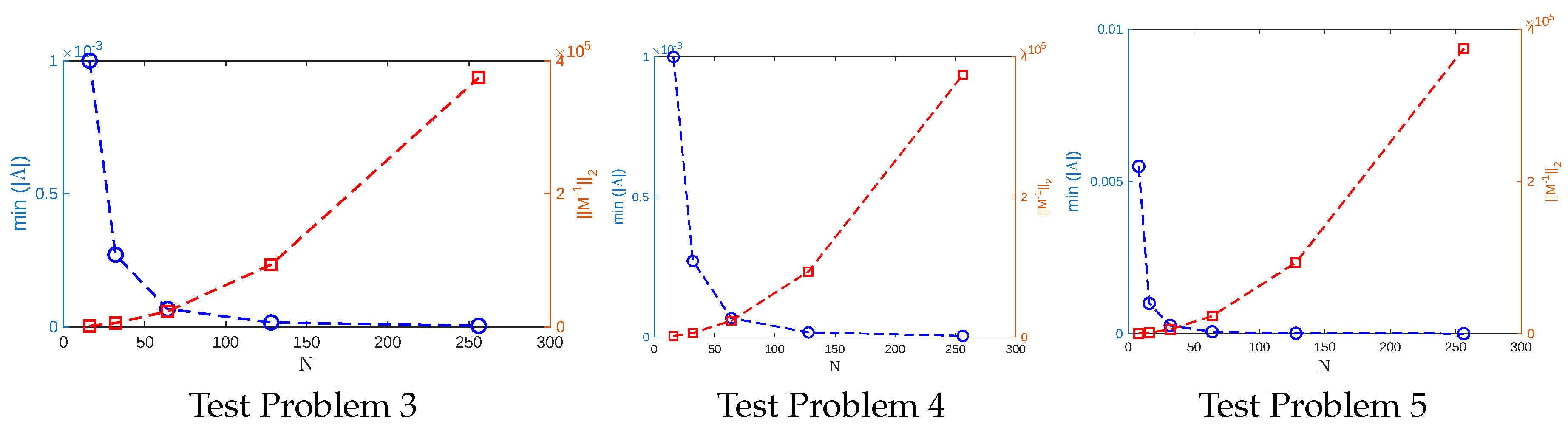
To investigate the stability of the proposed numerical scheme, we examine the spectral properties of the coefficient matrix $\mathrm{\Psi }$. Since the eigenvalues of ${\mathrm{\Psi }}^{-1}$ are given by the reciprocals of the corresponding eigenvalues of $\mathrm{\Psi }$, a bounded inverse requires the eigenvalues of $\mathrm{\Psi }$ to remain sufficiently separated from zero as the number of collocation points increases. Therefore, the smallest eigenvalue magnitude, ${\min }_{\lambda \in \sigma \left(\mathrm{\Psi }\right)}\left|\lambda \right|$, is employed as a diagnostic measure of numerical stability for both the linear and nonlinear test problems.

The numerical results presented in Figure 1 show that the minimum eigenvalue magnitude remains bounded away from zero as (N) increases. Consequently, the corresponding inverse matrices do not exhibit significant growth in their norm, indicating that the proposed HWCM formulation remains well-conditioned with respect to the refinement of the collocation grid. These observations provide numerical evidence supporting the stability of the proposed method.

7. Numerical Studies

In this section, we conduct an extensive set of numerical experiments to evaluate the capability of the proposed numerical strategy in terms of precision, computational efficiency, and implementable applicability. The constructed model developed is incorporated into Equation (39) specifically to handle multiple nonlinear test cases, demonstrating the method’s capability to deal with sophisticated and realistic cases. To rigorously examine the accuracy of the scheme, we compute the MAEs, $R_c\left(\mathfrak{M}\right)$ and RMSEs, under multiple discretization parameter choices $\mathfrak{M}$. These quantitative indicators provide a comprehensive evaluation of the solution’s precision and the method’s ability to estimate the exact or benchmark approximation effectively. The expressions used for computing the resulting errors metrics are given as follows:

$$\begin{array}{ccc}\hfill \mathrm{MAEs}& =& {\parallel {\phi }^{\mathrm{true}}-{\phi }^{\mathrm{approx}}\parallel }_{\infty }\approx \underset{j}{\max }\left|{\phi }_j^{\mathrm{true}}-{\phi }_j^{\mathrm{approx}}\right|,\hfill \end{array}$$

(43)

$$\begin{array}{ccc}\hfill \mathrm{RMSEs}& \approx & \sqrt{\left({\displaystyle \frac{1}{\mathfrak{M}}}\sum _{j=1}^{\mathfrak{M}}{\left({\phi }_j^{\mathrm{true}}-{\phi }_j^{\mathrm{approx}}\right)}^2\right)},\hfill \end{array}$$

(44)

and the computational rate of convergence is defined by

$$R_c\left(\mathfrak{M}\right)={\log }_2\left({\displaystyle \frac{E_{\mathfrak{M}}}{E_{\mathfrak{M}/2}}}\right)$$

where ${\phi }_j^{\mathrm{true}}$ represents the exact (analytical) solution at the j-th collocation point, and ${\phi }_j^{\mathrm{approx}}$ denotes the corresponding numerical approximation. The symbol $E_c\left(\mathfrak{M}\right)$ refers to the computed error for a given number of collocation points $\mathfrak{M}$.

These metrics allow for a comprehensive analysis of how well the numerical solution approximates the exact solution and how the accuracy improves as the discretization becomes finer. A higher rate of convergence $R_c\left(\mathfrak{M}\right)$ indicates that the method yields increasingly accurate results with refinement of the computational grid.

Test Problem 1.

Let us analyze the linear hyperbolic model with one interface, given by:

$${\phi }_{\mathfrak{t}\mathfrak{t}}(\sigma ,\mathfrak{t})={\left(\lambda \left(\sigma \right){\phi }_{\sigma }(\sigma ,\mathfrak{t})\right)}_{\sigma }+\psi (\sigma ,\mathfrak{t}),$$

(45)

with the exact solution:

$$\phi (\sigma ,\mathfrak{t})=\left\{\begin{array}{c}{\phi }_1(\sigma ,\mathfrak{t})={\displaystyle \frac{1}{3}}{\sigma }^{3}cos\left(\mathfrak{t}\right),0\le \sigma \le 0.5,\hfill \\ {\phi }_2(\sigma ,\mathfrak{t})={\sigma }^{3}cos\left(\mathfrak{t}\right),0.5\le \sigma \le 1,\hfill \end{array}\right.$$

and

$$\lambda \left(\sigma \right)=\left\{\begin{array}{c}{\lambda }_1\left(\sigma \right)=1,0\le \sigma \le 0.5,\hfill \\ {\lambda }_2\left(\sigma \right)=2,0.5\le \sigma \le 1,\hfill \end{array}\right.$$

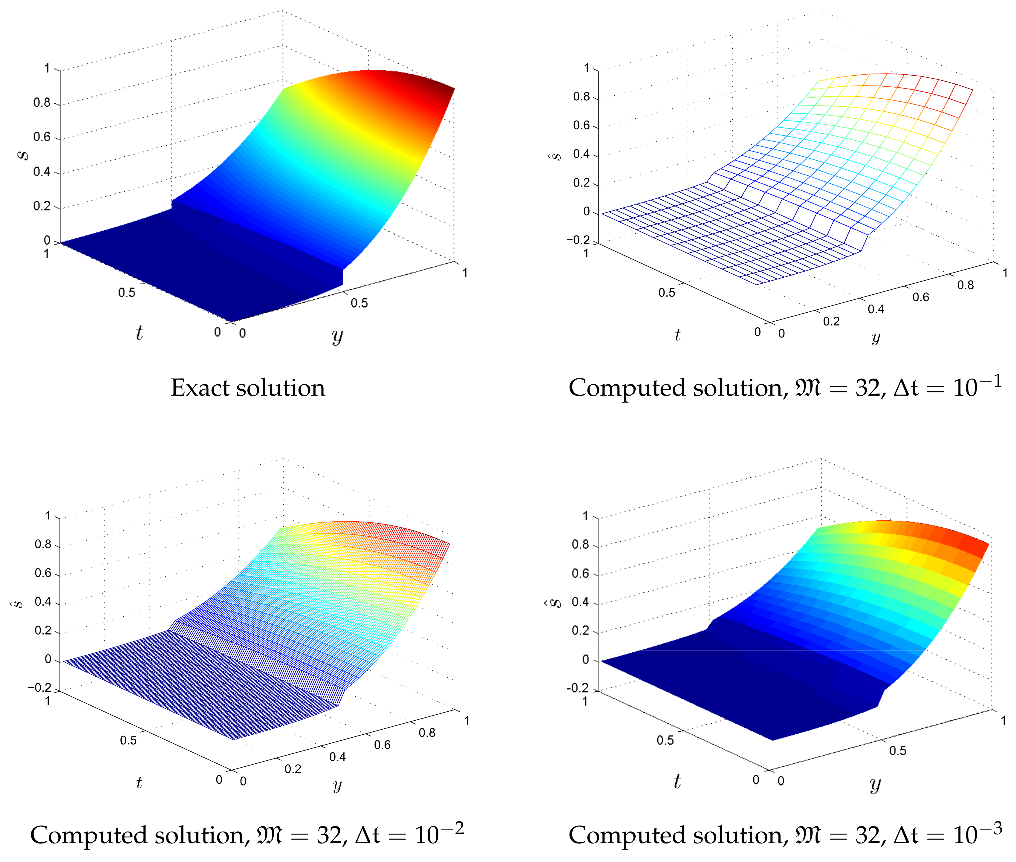
The exact solution is to define the boundary, interface and initial conditions. This test problem corresponds to a linear case. The numerical approach is employed for this problem, along with the computed results presented in

Table 1. Examination of computational errors in Test Problem 1.

dt	j	N	MAEs	RMSEs	CPU Time	${\mathit{R}}_{\mathit{c}}\mathbf{\left(}\mathfrak{M}\mathbf{\right)}$
$0.01/4$	0	4	$9.3000\times {10}^{-3}$	$6.7000\times {10}^{-3}$	0.0346	—
$0.01/8$	1	8	$2.5000\times {10}^{-3}$	$1.7000\times {10}^{-3}$	0.0496	1.8953
$0.01/16$	2	16	$6.3384\times {10}^{-4}$	$4.2838\times {10}^{-4}$	0.0498	1.9808
$0.01/32$	3	32	$1.5820\times {10}^{-4}$	$1.04046\times {10}^{-4}$	0.2185	2.0013
$0.01/64$	4	64	$3.8399\times {10}^{-5}$	$2.4390\times {10}^{-5}$	16.2805	2.0425

. The following table provides values for the MAEs, RMSEs, and the $R_c\left(\mathfrak{M}\right)$ for various numbers of CPs at distinct time step sizes. From the values shown in Table 1, it is observed that the MAEs are reduced to the order of ${10}^{-5}$, even with a relatively small number of CPs. Such accuracy is generally acceptable for practical purposes. The observed convergence rate approaches 2, which aligns well with theoretical predictions and previously published results [41,42]. Furthermore, more precise results can be obtained by increasing the concentration of the computational grid through a larger number of CPs. The comparison with MQ-RBF in

Table 2. Assessment of numerical errors in Test Problem 1 employing MQ-RBFs for $\Delta \tau =0.1$ with $\tau =1$.

$\mathit{\epsilon }\mathbf{=}\mathbf{2.5}$
$\mathit{N}$	MAEs	RMSEs	CPU Time (s)
4	$8.5600\times {10}^{-2}$	$6.0500\times {10}^{-2}$	0.017677
8	$2.0700\times {10}^{-2}$	$1.3100\times {10}^{-2}$	0.014940
12	$8.4000\times {10}^{-3}$	$5.5000\times {10}^{-3}$	0.002723
18	$1.4000\times {10}^{-3}$	$9.0722\times {10}^{-4}$	0.004070
20	$7.3007\times {10}^{-4}$	$4.3379\times {10}^{-4}$	0.002792

shows that the proposed Haar FDM scheme achieves higher accuracy with significantly smaller MAEs and RMSEs. Moreover, the Haar-based method reaches convergence with fewer collocation points. This confirms its computational efficiency and robustness over MQ-RBF for the first test case. Additionally, in Figure 2, a contrast of the estimate and true solutions is depicted visualized through 3D plots for multiple time step intervals, namely $\Delta \mathfrak{t}=0.1,0.01,0.001$, while fixing the number of CPs at $N=32$. These plots reveal a clearer understanding of the method’s effectiveness along with its error characteristics. The plotted outcomes presented in Figure 2 indicate a strong agreement between the estimate and true solutions. One of the central strengths of this hybrid scheme is its capability to reliably capture abrupt discontinuities at the interface, a feature that is graphically evident reflected in the computed results and 3D visualizations.

Test Problem 2.

The subsequent linear hyperbolic model, incorporating a single interface and variable coefficients, is examined:

$${\phi }_{\mathfrak{t}\mathfrak{t}}=\left\{\begin{array}{c}{\lambda }_1\left(\sigma \right){\phi }_{1\sigma \sigma }+{\psi }_1(\sigma ,\mathfrak{t}),0\le \sigma \le 0.5,\hfill \\ {\lambda }_2\left(\sigma \right){\phi }_{2\sigma \sigma }+{\psi }_2\left(\mathfrak{t}\mathfrak{t}\right),0.5\le \sigma \le 1,\hfill \end{array}\right.$$

with the exact solution:

$$\phi (\sigma ,\mathfrak{t})=\left\{\begin{array}{c}{\phi }_1(\sigma ,\mathfrak{t})=\sigma cos\left(\mathfrak{t}\right),0\le \sigma \le 0.5,\hfill \\ {\phi }_2(\sigma ,\mathfrak{t})=(\sigma +{\displaystyle \frac{1}{2}})cos\left(\mathfrak{t}\right),0.5\le \sigma \le 1,\hfill \end{array}\right.$$

and

$$\lambda \left(\sigma \right)=\left\{\begin{array}{c}{\lambda }_1\left(\sigma \right)={\displaystyle \frac{\sigma }{3}},0\le \sigma \le 0.5,\hfill \\ {\lambda }_2\left(\sigma \right)=\sigma ,0.5\le \sigma \le 1,\hfill \end{array}\right.$$

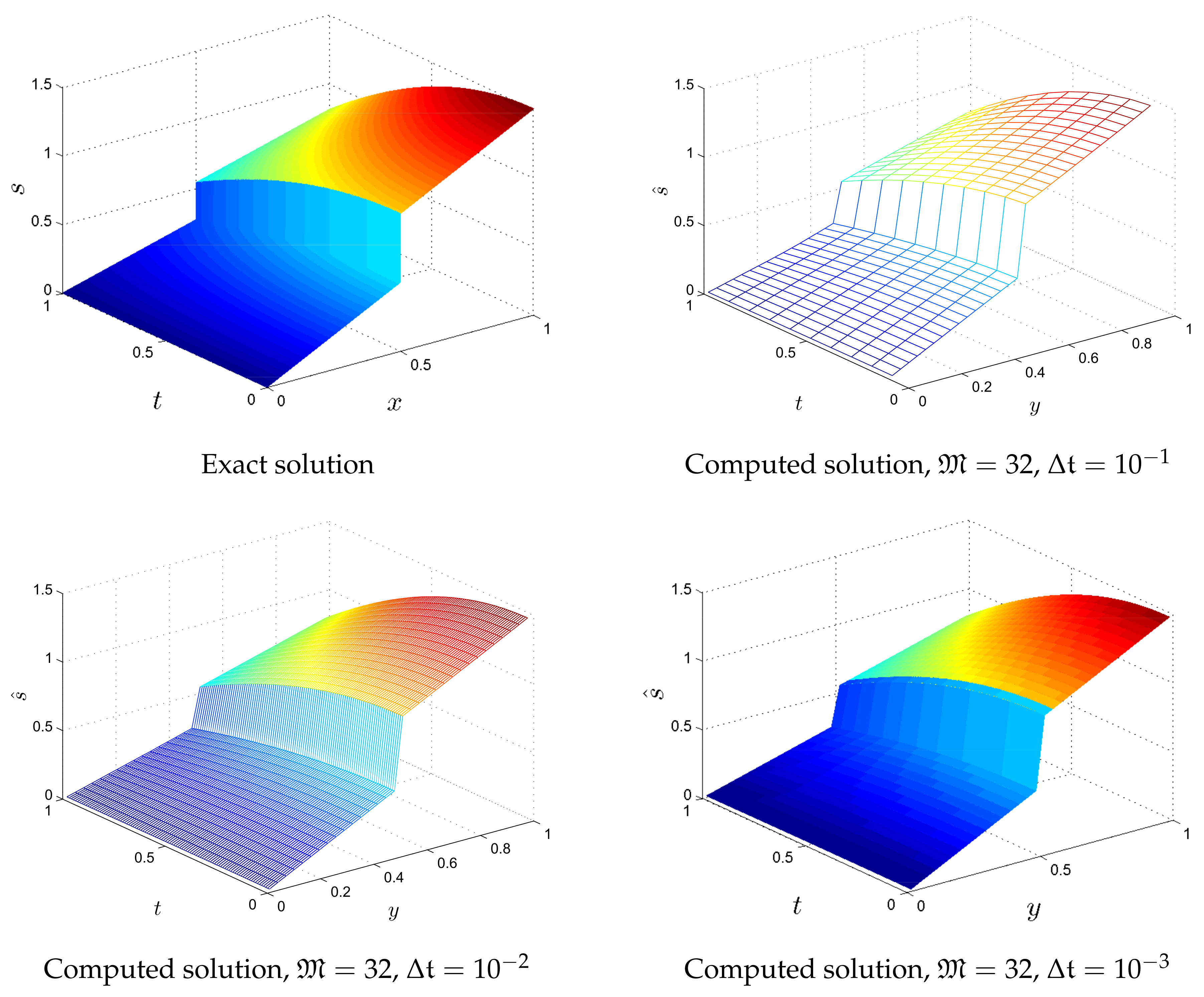
The exact solution is utilized to define the boundary, interface, and initial conditions for this test problem, which corresponds to a linear case. The proposed numerical method is further utilized in this problem, and the resulting simulation data are summarized in

Table 3. Evaluation of computing errors in Test Problem 2.

dt	j	N	MAEs	RMSEs	CPU Time	${\mathit{R}}_{\mathit{c}}\mathbf{\left(}\mathfrak{M}\mathbf{\right)}$
$0.01/4$	0	4	$4.4090\times {10}^{-4}$	$2.8274\times {10}^{-4}$	0.169610	—
$0.01/8$	1	8	$2.9202\times {10}^{-4}$	$1.2620\times {10}^{-4}$	0.172861	0.6048
$0.01/16$	2	16	$1.5305\times {10}^{-4}$	$6.3702\times {10}^{-5}$	0.193140	0.9321
$0.01/32$	3	32	$8.8187\times {10}^{-5}$	$3.1959\times {10}^{-5}$	0.395092	0.9026
$0.01/32$	4	64	$4.1781\times {10}^{-5}$	$1.5946\times {10}^{-5}$	2.010987	0.9705

. The computed RMSEs, MAEs and $R_c\left(\mathfrak{M}\right)$ are summarized in Table 3 for various numbers of CPs and different time step intervals. From the data in Table 3, it can be seen that the MAEs decrease to the order of ${10}^{-5}$, even with a relatively small number of CPs, demonstrating the efficiency and efficiency of the scheme. Such precision is generally considered sufficient for practical applications. More precise results are attainable by growing the density of the computational grid through the use of a greater number of CPs. As shown in Table 3 and

Table 4. Assessment of numerical errors in Test Problem 2 employing MQ-RBFs for $\Delta \tau =0.1$ with $\tau =1$.

$\mathit{\epsilon }\mathbf{=}\mathbf{2}$
$\mathit{N}$	MAEs	RMSEs	CPU Time (s)
2	$1.5830\times {10}^{-1}$	$1.1190\times {10}^{-1}$	0.014154
4	$7.8600\times {10}^{-2}$	$5.6500\times {10}^{-2}$	0.008559
10	$1.2100\times {10}^{-2}$	$7.6000\times {10}^{-3}$	0.006723
16	$1.8000\times {10}^{-3}$	$8.3680\times {10}^{-4}$	0.006121
22	$9.1801\times {10}^{-4}$	$4.0057\times {10}^{-4}$	0.009908

, when compared with MCM and HWCM, the proposed approach produces lower error margins and higher accuracy, demonstrating its reliability in solving the test problem efficiently. Additionally, Figure 3 presents a plotted assessment among the exact and computed solution utilizing 3D plots for various time step sizes, namely $\Delta \mathfrak{t}={10}^{-1},{10}^{-2},{10}^{-3}$, while keeping the number of CPs fixed at $N=32$. The results are further evaluated against the MCM reported in the literature. This comparison demonstrates that the proposed scheme provides enhanced efficiency and improved accuracy for the hyperbolic model with a single interface, outperforming previously established approaches. These visualizations provide further understanding of the efficiency and error characteristics regarding the suggested approach. The plotted outcomes shown in Figure 3 reveal a strong agreement contrasting the predicted and analytical solutions. The 3D visualization clearly demonstrates that the proposed computational scheme has effectively captured all the critical features of this complex interface case. The scheme not only solves the primary solution dynamics with high accuracy but also accurately tracks the intricate variations and the sudden variations observed at the interface. The illustrated results reinforce the robustness and reliability of the approach in handling challenging interface cases, that are often difficult to model using conventional numerical schemes.

Test Problem 3.

Let us analyze the linear hyperbolic model with a single interface, described as follows:

$${\phi }_{\mathfrak{t}\mathfrak{t}}(\sigma ,\mathfrak{t})=\left\{\begin{array}{cc}{\phi }_{1\sigma \sigma }(\sigma ,\mathfrak{t})+{\psi }_1(\sigma ,\mathfrak{t}),\hfill & 0\le \sigma \le 0.5,\hfill \\ 2{\phi }_{2\sigma \sigma }(\sigma ,\mathfrak{t})+{\psi }_1(\sigma ,\mathfrak{t}),\hfill & 0.5\le \sigma \le 1,\hfill \end{array}\right.$$

with the exact solution:

$$\phi (\sigma ,\mathfrak{t})=\left\{\begin{array}{c}{\phi }_1(\sigma ,\mathfrak{t})={\sigma }^8{e}^{-\mathfrak{t}},0\le \sigma \le 0.5,\hfill \\ {\phi }_2(\sigma ,\mathfrak{t})={\displaystyle \frac{1}{2}}({\sigma }^8+{\displaystyle \frac{1}{256}})e^{-\mathfrak{t}},0.5\le \sigma \le 1,\hfill \end{array}\right.$$

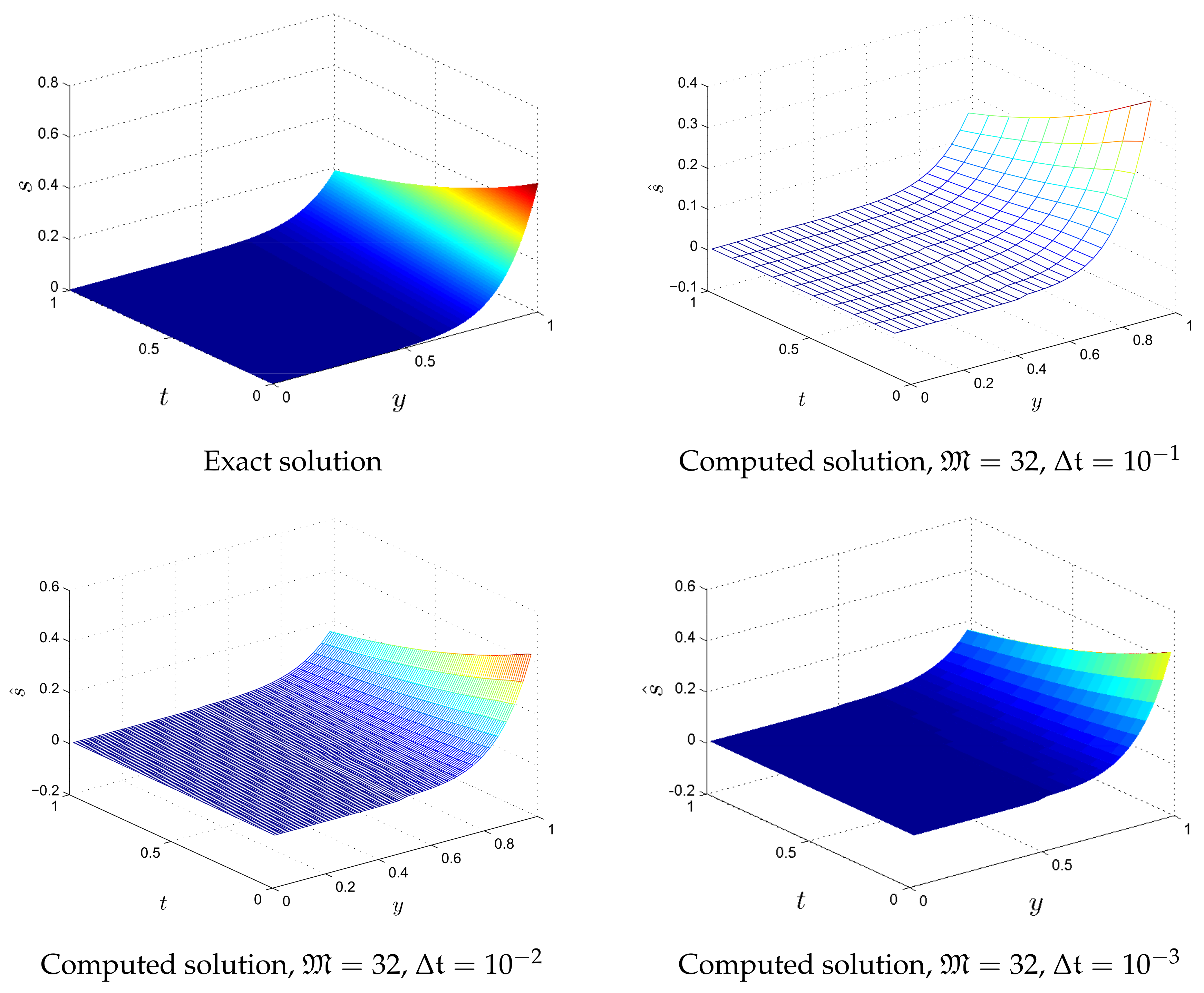
The source function, as well as the boundary, interface, and initial conditions, are defined using the exact solution. This numerical experiment addresses a linear hyperbolic model, for which the suggested computational approach is employed to obtain the solution. Table 3 presents the MAEs, RMSEs, and the estimated convergence rates. The observed convergence rate consistently approaches a value of 2, which strongly supports the theoretical expectations for second-order accurate methods. This result not only validates the underlying numerical formulation but also demonstrates the reliability and robustness of the proposed scheme. Furthermore, the observed convergence trend shows strong agreement with previously reported findings in the literature [41,42], thereby reinforcing the method’s credibility and alignment with established numerical analysis benchmarks. The results demonstrate a consistent reduction in error as the number of collocation points increases and the time step size decreases, confirming the method’s accuracy and convergence behavior. In comparison with MCM and HWCM as presented in

Table 5. Evaluation of numerical errors in Test Problem 3.

dt	j	N	MAEs	RMSEs	CPU Time	${\mathit{R}}_{\mathit{c}}\mathbf{\left(}\mathfrak{M}\mathbf{\right)}$
$0.01/4$	0	4	$3.0900\times {10}^{-2}$	$2.3300\times {10}^{-2}$	0.189007	—
$0.01/8$	1	8	$1.0500\times {10}^{-2}$	$7.3000\times {10}^{-3}$	0.193126	1.5557
$0.01/16$	2	16	$2.9000\times {10}^{-3}$	$1.9000\times {10}^{-3}$	0.194190	1.8563
$0.01/32$	3	32	$7.1476\times {10}^{-4}$	$4.8799\times {10}^{-4}$	0.348029	2.0205
$0.01/64$	4	64	$1.7826\times {10}^{-4}$	$1.2152\times {10}^{-4}$	1.721865	2.0035

and

Table 6. Assessment of numerical errors in Test Problem 3 employing MQ-RBFs for $\Delta \tau =0.5$ with $\tau =1$.

$\mathit{\epsilon }\mathbf{=}\mathbf{2.2}$
$\mathit{N}$	MAEs	RMSEs	CPU Time (s)
2	$8.5600\times {10}^{-2}$	$6.0500\times {10}^{-2}$	0.011859
4	$1.6800\times {10}^{-2}$	$9.2000\times {10}^{-3}$	0.013385
12	$7.3000\times {10}^{-3}$	$4.5000\times {10}^{-3}$	0.004973
20	$4.1613\times {10}^{-4}$	$2.9514\times {10}^{-4}$	0.004792
24	$4.9861\times {10}^{-4}$	$2.4452\times {10}^{-4}$	0.006795

, the proposed method attains reduced error levels and improved accuracy, underscoring its strong capability to resolve the test problem with high precision. Moreover, Figure 4 provides surface plots that visually compare the computed and exact solutions at various time levels. These graphical illustrations offer clear evidence of the method’s effectiveness in accurately resolving the solution structure and capturing the essential features of the interface dynamics.

Test Problem 4.

Let us analyze the nonlinear hyperbolic model incorporating a single interface, described below:

$${\phi }_{\mathfrak{t}\mathfrak{t}}(\sigma ,\mathfrak{t})=\left\{\begin{array}{c}{\phi }_{1\sigma \sigma }(\sigma ,\mathfrak{t})+2{\phi }_1^2(\sigma ,\mathfrak{t})+{\psi }_1(\sigma ,\mathfrak{t}),0\le \sigma \le 0.5,\hfill \\ 2{\phi }_{2\sigma \sigma }(\sigma ,\mathfrak{t})+2{\phi }_2^2(\sigma ,\mathfrak{t})+{\psi }_1(\sigma ,\mathfrak{t}),0.5\le \sigma \le 1,\hfill \end{array}\right.$$

with the exact solution:

$$\phi (\sigma ,\mathfrak{t})=\left\{\begin{array}{c}{\phi }_1(\sigma ,\mathfrak{t})={\sigma }^4{e}^{-\mathfrak{t}},0\le \sigma \le 0.5,\hfill \\ {\phi }_2(\sigma ,\mathfrak{t})={\displaystyle \frac{1}{2}}({\sigma }^4+{\displaystyle \frac{1}{16}})e^{-\mathfrak{t}},0.5\le \sigma \le 1,\hfill \end{array}\right.$$

Boundary, interface, and initial conditions are determined directly from the exact solution. This numerical experiment addresses a nonlinear problem, for which the proposed computational approach is employed to obtain the solution.

Table 7. Assessment of numerical errors in Test Problem 4.

dt	j	N	MAEs	RMSEs	CPU Time	${\mathit{R}}_{\mathit{c}}\mathbf{\left(}\mathfrak{M}\mathbf{\right)}$
$0.01/4$	0	4	$4.2000\times {10}^{-3}$	$3.0000\times {10}^{-3}$	0.006395	—
$0.01/8$	1	8	$1.2000\times {10}^{-3}$	$8.5105\times {10}^{-4}$	0.009641	1.8074
$0.01/16$	2	16	$2.9179\times {10}^{-4}$	$2.1043\times {10}^{-4}$	0.021175	2.0400
$0.01/32$	3	32	$7.6891\times {10}^{-5}$	$5.2160\times {10}^{-5}$	0.163725	1.9241
$0.01/64$	4	64	$4.6539\times {10}^{-5}$	$1.6534\times {10}^{-5}$	1.325789	0.7244

presents the MAEs, RMSEs, and the estimated convergence rates. The observed convergence rate consistently approaches a value of 2, which strongly supports the theoretical expectations for second-order accurate methods. This result not only validates the underlying numerical formulation but also demonstrates the reliability and robustness of the proposed scheme. As shown in Table 7 and

Table 8. Assessment of numerical errors in Benchmark Example 4 employing MQ-RBFs for $\Delta \tau =0.001$ with $\tau =1$.

$\mathit{\epsilon }\mathbf{=}\mathbf{2}$
F	${\mathit{E}}_{\mathit{c}}\mathbf{\left(}\mathit{F}\mathbf{\right)}$	RMSEs
4	$1.1200\times {10}^{-2}$	$7.5000\times {10}^{-3}$
8	$4.3000\times {10}^{-3}$	$2.3000\times {10}^{-3}$
16	$2.5000\times {10}^{-3}$	$1.3000\times {10}^{-3}$
20	$2.2000\times {10}^{-3}$	$1.2000\times {10}^{-3}$
24	$2.0000\times {10}^{-4}$	$1.0000\times {10}^{-4}$

, when compared with MCM and HWCM, the proposed approach produces lower error margins and higher accuracy, demonstrating its reliability in solving the test problem efficiently. Furthermore, the observed convergence trend is in close agreement with previously reported findings in References [41,42], thereby reinforcing the method’s credibility and alignment with established numerical analysis benchmarks. When extended to nonlinear cases, the proposed method continues to provide accurate and reliable solutions, effectively addressing nonlinearity.

Test Problem 5.

Let us focus on the nonlinear hyperbolic model with a single interface, given by:

$${\phi }_{\mathfrak{t}\mathfrak{t}}=\left\{\begin{array}{c}{\phi }_{1\sigma \sigma }+2{\phi }_1^2(\sigma ,\mathfrak{t})+{\psi }_1(\sigma ,\mathfrak{t}),0\le \sigma \le 0.5,\hfill \\ 2{\phi }_{2\sigma \sigma }+2{\phi }_2^2(\sigma ,\mathfrak{t})+{\psi }_2(\sigma ,\mathfrak{t}),0.5\le \sigma \le 1,\hfill \end{array}\right.$$

with the exact solution:

$$\phi (\sigma ,\mathfrak{t})=\left\{\begin{array}{c}{\phi }_1(\sigma ,\mathfrak{t})={\displaystyle \frac{\sigma }{3}}cos\left(\mathfrak{t}\right),0\le \sigma \le 0.5,\hfill \\ {\phi }_2(\sigma ,\mathfrak{t})=\sigma cos\left(\mathfrak{t}\right),0.5\le \sigma \le 1,\hfill \end{array}\right.$$

The exact solution is utilized to define the boundary, interface, and initial conditions. This example presents another nonlinear interface model to further validate the effectiveness of the suggested numerical approach. The same numerical approach has been applied to this model as well. The corresponding numerical results, including the RMSEs, MAEs, and the $R_c\left(\mathfrak{M}\right)$, are summarized in

Table 9. Quantitative assessment of numerical errors in Test Problem 5.

j	N	dt	MAEs	RMSEs	CPU Time	${\mathit{R}}_{\mathit{c}}\mathbf{\left(}\mathfrak{M}\mathbf{\right)}$
$0.01/4$	0	4	$1.6624\times {10}^{-4}$	$1.3060\times {10}^{-4}$	0.015277	—
$0.01/8$	1	8	$9.2316\times {10}^{-5}$	$6.2406\times {10}^{-5}$	0.019191	0.8486
$0.01/16$	2	16	$4.8669\times {10}^{-5}$	$3.1024\times {10}^{-5}$	0.094088	0.9236
$0.01/32$	3	32	$2.4528\times {10}^{-5}$	$1.5509\times {10}^{-5}$	0.689951	0.9885
$0.01/64$	4	64	$1.2252\times {10}^{-5}$	$7.7619\times {10}^{-6}$	6.909698	1.0014

. As shown in Table 9 and

Table 10. Assessment of numerical errors in Test Problem 5 employing MQ-RBFs for $\Delta \tau =0.5$ with $\tau =1$.

$\mathit{\epsilon }\mathbf{=}\mathbf{2.5}$
$\mathit{N}$	MAEs	RMSEs
4	$6.5400\times {10}^{-2}$	$4.4200\times {10}^{-2}$
6	$3.5500\times {10}^{-2}$	$2.4000\times {10}^{-2}$
8	$2.3000\times {10}^{-3}$	$1.5700\times {10}^{-3}$
14	$1.2600\times {10}^{-4}$	$8.9000\times {10}^{-4}$
16	$1.2300\times {10}^{-4}$	$8.7000\times {10}^{-4}$

, when compared with MCM and HWCM, the proposed approach produces lower error margins and higher accuracy, demonstrating its reliability in solving the test problem efficiently. A careful examination of the results in the table reveals a notable improvement in accuracy, thereby reinforcing the efficiency and robustness of the method in handling nonlinear problems. It is observed that the convergence rate decreases to approximately 0.72 in Examples 4 and 5. This reduction is mainly associated with the presence of interface discontinuities and the increased complexity of the underlying problems. Despite this decrease, the numerical results remain stable and confirm the effectiveness of the proposed method for the considered interface problems.

8. Conclusions

In this study, we have proposed and implemented a hybrid numerical approach that combines the FDM with the HWCM to efficiently solve one-dimensional hyperbolic interface problems. The proposed approach has been applied to a variety of linear and nonlinear models involving both variable and constant coefficients. The comparative study, carried out on three linear and two nonlinear benchmark problems, highlights the advantage of HWCM over MCM in terms of accuracy. Despite this, the HWCM framework proves to be computationally demanding, requiring longer execution time. In contrast, MCM achieves results with lower accuracy but at a significantly reduced computational cost. One of the central strengths of this hybrid scheme is its capability to accurately capture sharp discontinuities at the interface, a feature that is graphically evident in the numerical results and 3D visualizations. The hybrid nature of the method leverages the stability and simplicity of FDM along with the multi-resolution accuracy and compact support of the Haar wavelets. This combination ensures improved numerical performance, ease of implementation, and adaptability to different problem types. The results show that the scheme is not only computationally efficient but also capable of producing highly accurate solutions even in the presence of complex interface behavior. A detailed numerical analysis was carried out using various CPs. The computed MAEs, RMSEs, and experimental rates of convergence consistently show that the reliability of the scheme improves with an increase in the number of collocation points. For most test cases, the observed convergence rate approaches 2, which aligns well with theoretical predictions and previously published results [41,42]. In the numerical experiments, the spatial resolution and time step are generally refined simultaneously; therefore, the observed convergence rates reflect the combined space-time discretization errors and should not be interpreted as an independent verification of the third-order spatial accuracy. Thus, rates closer to two may result from the influence of the temporal discretization error. Overall, the proposed FDM-HWCM hybrid strategy is validated as a reliable and powerful tool for addressing hyperbolic interface problems with high accuracy, efficiency, and excellent interface-capturing capabilities. In future research, we plan to employ the Higher-Order Haar Wavelet Collocation Method [43] to solve interface problems with improved accuracy and extend this methodology to fractional interface problems, which are increasingly important for modeling physical systems involving memory and nonlocal effects. Specifically, we aim to address single and double interface problems governed by fractional PDEs. The establishment of efficient and accurate numerical methods for such problems remains an open and challenging area.

References

1. Mohyud-Din, S.T.; Yildirim, A.; Kaplan, Y. Homotopy perturbation method for one-dimensional hyperbolic equation with integral conditions. Z. Naturforsch. A 2010, 65, 1077–1080. [Google Scholar] [CrossRef] [Scilit]
2. Aziz, I.; Nisar, M. On the numerical solution of some differential equations with nonlocal integral boundary conditions via Haar wavelet. Proc. Est. Acad. Sci. 2022, 71, 30–54. [Google Scholar] [CrossRef] [Scilit]
3. Zaman, S.S.; Amin, R.; Haider, N.; Akgül, A. Numerical solution of Fisher’s equation through the application of Haar wavelet collocation method. Numer. Heat Transf. Part B Fundam. 2025, 86, 2746–2757. [Google Scholar] [CrossRef] [Scilit]
4. Fahim, M.; Asif, M.; Haider, N.; Amin, R. Hybrid Haar wavelet and meshfree methods for hyperbolic double interface problems: Numerical implementations and comparative performance analysis. Part. Diff. Eqn. Appl. Math. 2024, 11, 100773. [Google Scholar] [CrossRef] [Scilit]
5. Liu, W.K.; Liu, Y.; Farrell, D.; Zhang, L.; Wang, S.; Fukui, Y.; Patankar, N.; Zhang, Y.; Bajaj, C.; Hong, J.L. Immersed finite element method and its applications to biological systems. Comput. Methods Appl. Mech. Eng. 2006, 195, 1722–1749. [Google Scholar] [CrossRef] [Scilit] [PubMed]
6. Adel, M.; Khader, M.M.; Babatin, M.M.; Youssef, M.Z. Numerical investigation for the fractional model of pollution for a system of lakes using the SCM based on the Appell type Changhee polynomials. AIMS Math. 2023, 8, 31104–31117. [Google Scholar] [CrossRef] [Scilit]
7. Li, Z.; Ito, K. The Immersed Interface Methods: Numerical Solution of PDEs Involving Interfaces and Irregular Domains; Society for Industrial and Applied Mathematics: Philadelphia, PA, USA, 2006. [Google Scholar]
8. Ahmed, A.F.S.; Gamal, I.; Abdelrahman, M.; AbdEl-Bar, M. Derivation of an approximate formula of the Rabotnov fractional-exponential kernel fractional derivative and applied for numerically solving the blood ethanol concentration system. AIMS Math. 2023, 8, 30704–30716. [Google Scholar] [CrossRef] [Scilit]
9. Epshteyn, Y.; Phippen, S. High-order difference potentials methods for 1D elliptic type models. Appl. Numer. Math. 2015, 93, 69–86. [Google Scholar] [CrossRef] [Scilit]
10. Peskin, C.S. Numerical analysis of blood flow in the heart. J. Comput. Phys. 1977, 25, 220–252. [Google Scholar] [CrossRef] [Scilit]
11. Peskin, C.S. The immersed boundary method. Acta Numer. 2002, 11, 479–517. [Google Scholar] [CrossRef] [Scilit]
12. Fedkiw, R.P.; Aslam, T.; Merriman, B.; Osher, S. A Non-oscillatory Eulerian approach to interfaces in multimaterial flows (the Ghost Fluid Method). J. Comput. Phys. 1999, 152, 457–492. [Google Scholar] [CrossRef] [Scilit]
13. Liu, X.-D.; Sideris, T.C. Convergence of the ghost fluid method for elliptic equations with interfaces. Math. Comput. 2003, 72, 1731–1746. [Google Scholar] [CrossRef] [Scilit]
14. Liu, X.-D.; Fedkiw, R.P.; Kang, M. A boundary condition capturing method for Poisson’s equation on irregular domains. J. Comput. Phys. 2000, 160, 151–178. [Google Scholar] [CrossRef] [Scilit]
15. Randall, J.L.; LeVeque; Zhilin. The immersed interface method for elliptic equations with discontinuous coefficients and singular sources. SIAM J. Numer. Anal. 1994, 31, 1019–1044. [Google Scholar] [CrossRef] [Scilit]
16. Zhou, S.Y.; Wei, G.W. Matched interface and boundary (MIB) method for elliptic problems with sharp-edged interfaces. J. Comput. Phys. 2007, 224, 729–756. [Google Scholar] [CrossRef] [Scilit]
17. Zhou, Y.C.; Liu, J.; Harry, D.L. A matched interface and boundary method for solving multi-flow Navier-Stokes equations with applications to geodynamics. J. Comput. Phys. 2012, 231, 223–242. [Google Scholar] [CrossRef] [Scilit]
18. Zhou, Y.C.; Zhao, S.; Feig, M.; Wei, G.W. High order matched interface and boundary method for elliptic equations with discontinuous coefficients and singular sources. J. Comput. Phys. 2006, 213, 1–30. [Google Scholar] [CrossRef] [Scilit]
19. Aziz, I.; Islam, S.; Haider, N. Meshless and multi-resolution collocation techniques for steady state interface models. Int. J. Comput. Methods 2018, 15, 1750073. [Google Scholar] [CrossRef] [Scilit]
20. Aziz, I.; Islam, S.; Haider, N. Meshless and multi-resolution collocation techniques for parabolic interface models. Appl. Math. Comput. 2018, 335, 313–332. [Google Scholar] [CrossRef] [Scilit]
21. Matthew, A. On finite element method for linear hyperbolic interface problems. J. Niger. Math. Soc. 2018, 37, 41–55. [Google Scholar]
22. Rana, G.; Asif, M.; Haider, N.; Bilal, R.; Ahsan, M.; Al-Mdallal, Q.; Jarad, F. A modified algorithm based on Haar wavelets for the numerical simulation of interface models. J. Funct. Spaces 2022, 2022, 1541486. [Google Scholar] [CrossRef] [Scilit]
23. Asif, M.; Farooq, U.; Riaz, B.; Bilal, F.; Haider, N. Numerical assessment of hyperbolic type double interface problems via Haar wavelets. Part. Differ. Equ. Appl. Math. 2024, 10, 100665. [Google Scholar] [CrossRef] [Scilit]
24. Kelin, X.; Meng, Z.; Guo-Wei, W.; Galerkin, M.I.B. Method for elliptic interface problems. J. Comput. Appl. Math. 2014, 272, 195–220. [Google Scholar] [CrossRef] [Scilit] [PubMed]
25. Chen, Z.; Zou, Z. Finite element methods and their convergence for elliptic and parabolic interface problems. Numer. Math. 1998, 79, 175–202. [Google Scholar] [CrossRef] [Scilit]
26. Masood, A.; Baseer, A.; Islam, S. Local radial basis function collocation method for Stokes equations with interface conditions. Eng. Anal. Bound. Elem. 2020, 119, 246–256. [Google Scholar] [CrossRef] [Scilit]
27. Masood, A.; Elisabeth, L. Local meshless methods for second order elliptic interface problems with sharp corners. J. Comput. Phys. 2020, 416, 109599. [Google Scholar] [CrossRef] [Scilit]
28. Asif, M.; Gul, T.; Riaz, M.B.; Bilal, F. Solution of nonlinear telegraph equation with discontinuities along the transmission line using meshless collocation method. Part. Differ. Equ. Appl. Math. 2025, 14, 101219. [Google Scholar] [CrossRef] [Scilit]
29. Asif, M.; Bilal, F.; Bilal, R.; Shakeel, M. An efficient algorithm for the numerical solution of telegraph interface model with discontinuous coefficients via Haar wavelets. Alex. Eng. J. 2023, 72, 275–285. [Google Scholar] [CrossRef] [Scilit]
30. Asif, M.; Haider, N.; Al-Mdallal, Q.; Khan, I. A Haar wavelet collocation approach for solving one and two-dimensional second-order linear and nonlinear hyperbolic telegraph equations. Numer. Methods Part. Differ. Equ. 2020, 36, 1962–1981. [Google Scholar] [CrossRef] [Scilit]
31. Maleknejad, K.; Lotfi, T.; Mahdiani, K. Numerical solution of first kind Fredholm integral equations with wavelets-Galerkin method (WGM) and wavelets precondition. Appl. Math. Comput. 2007, 186, 794–800. [Google Scholar] [CrossRef] [Scilit]
32. Amin, R.; Shah, K.; Awais, M.; Ibrahim, M.; Sooppy, K.; Wojciech, S. Existence and solution of third-order integro-differential equations via Haar wavelet method. Fractals 2023, 31, 2340037. [Google Scholar] [CrossRef] [Scilit]
33. Wu, J. A wavelet operational method for solving fractional partial differential equations numerically. Appl. Math. Comput. 2009, 214, 31–40. [Google Scholar] [CrossRef] [Scilit]
34. Amin, R.; Hadi, F.; Altanji, M.; Sooppy, K.; Wojciech, S. Solution of variable-order nonlinear fractional differential equations using Haar wavelet collocation technique. Fractals 2023, 31, 2340022. [Google Scholar] [CrossRef] [Scilit]
35. Hajji, M.; Melkonian, S.; Vaillancourt, R. Representation of differential operators in wavelet basis. Comput. Math. Appl. 2004, 47, 1011–1033. [Google Scholar] [CrossRef] [Scilit]
36. Comincioli, V.; Naldi, G.; Scapolla, T. A wavelet-based method for numerical solution of nonlinear evolution equations. Appl. Numer. Math. 2000, 33, 291–297. [Google Scholar] [CrossRef] [Scilit]
37. Asif, M.; Akhtar, N.; Khan, F.; Bilal, F.; Popa, I.-L. Numerical treatment of hyperbolic-type problems with single and double interfaces via meshless method. Axioms 2025, 14, 621. [Google Scholar] [CrossRef] [Scilit]
38. Ahsan, M.; Tran, T.; Hussain, I.; Shakeel, M. A multiresolution collocation method and its convergence for Burgers’ type equations. Math. Meth. Appl. Sci. 2023, 46, 11702–11725. [Google Scholar] [CrossRef] [Scilit]
39. Sun, H.; Mei, L.; Lin, Y. New algorithm based on improved legendre orthonormal basis for solving second-order bvps. Appl. Math. Lett. 2021, 112, 106732. [Google Scholar] [CrossRef] [Scilit]
40. LeVeque, R.J. Finite Difference Methods for Ordinary and Partial Differential Equations; Society for Industrial and Applied Mathematics (SIAM): Philadelphia, PA, USA, 2007. [Google Scholar]
41. Majak, J.; Shvartsman, B.S.; Henrik, H. Convergence theorem for the Haar wavelet based discretization method. Compos. Struct. 2015, 126, 227–232. [Google Scholar] [CrossRef] [Scilit]
42. Majak, J.; Shvartsman, B.S.; Henrik, H. On the accuracy of the Haar wavelet discretization method. Compos. Part B Eng. 2015, 180, 321–327. [Google Scholar] [CrossRef] [Scilit]
43. Majak, J.; Pohlak, M.; Karjust, K.; Eerme, M.; Kurnitski, J.; Shvartsman, B.S. New higher order Haar wavelet method: Application to FGM structures. Compos. Strict. 2018, 201, 72–78. [Google Scholar] [CrossRef] [Scilit]
Figure 1. The stability analysis of the proposed method for linear and nonlinear test problems.
Mca 31 00197 g001
Figure 2. Study of the variation between analytical and computed solutions in Test Problem 1.
Mca 31 00197 g002
Figure 3. Quantitative evaluation of discrepancies between analytical and numerical solutions in Test Problem 2.
Mca 31 00197 g003
Figure 4. Analysis of numerical errors relative to the exact solution in Test Problem 3.
Mca 31 00197 g004