Hybridizing of Multi-Objective Coronavirus Herd Immunity Optimizer with Lévy Flight for Time Scheduling of Internet of Things Appliances in Smart Homes

Abstract

With the rapid deployment of Internet of Things appliances in smart homes, making efficient energy scheduling is a critical necessity to satisfy their exponentially increased residential energy demand. The problem of optimizing appliance operational times in smart homes is known as the Appliance Energy Scheduling Problem, which is a complex, NP-hard multi- objective challenge. Various metaheuristic algorithms have been utilized by researchers to address this problem; existing methods often struggle with slow convergence rates and are trapped in local optima. To overcome these limitations and produce a superior solution, this study proposes a new hybrid framework that integrates the Coronavirus Herd Immunity Optimizer (CHIO) with Lévy Flight (LF). By strategically embedding LF into the CHIO framework, the proposed method effectively balances exploration and exploitation search capabilities to achieve true global optimization. In the evaluation stage, three structural variations in hybrid CHIO models are evaluated against the standard appliance energy scheduling problem to determine the robust model and compare its performance with prominent existing methods in the literature. The experimental results demonstrate the superiority of the optimized CHIOLF-2 approach among other hybrid CHIO models. The CHIOLF-2 successfully navigates the trade-off between grid efficiency and user experience by achieving a reduction in electricity bills and the Peak-to-Average Ratio while maximizing user comfort through minimized appliance waiting times. Eventually, this research produces a highly efficient scheduling framework for modern smart homes and offers a versatile algorithmic design that can be readily adapted to address other complex real-world optimization problems.

1. Introduction

The transition of traditional power grids to the Smart Grid (SG) provides an intelligence-driven environment by managing the increasing energy demand actively and peak-load pressures through Internet of Things (IoT) smart homes [1,2,3]. Central to this ecosystem is the Energy Management Controller (EMC), which facilitates bidirectional communication between Energy Supplier Companies (ESCs) and households, enabling dynamic pricing schemes like Real-Time Pricing (RTP) and Inclining Block Rate (IBR) [4,5,6].

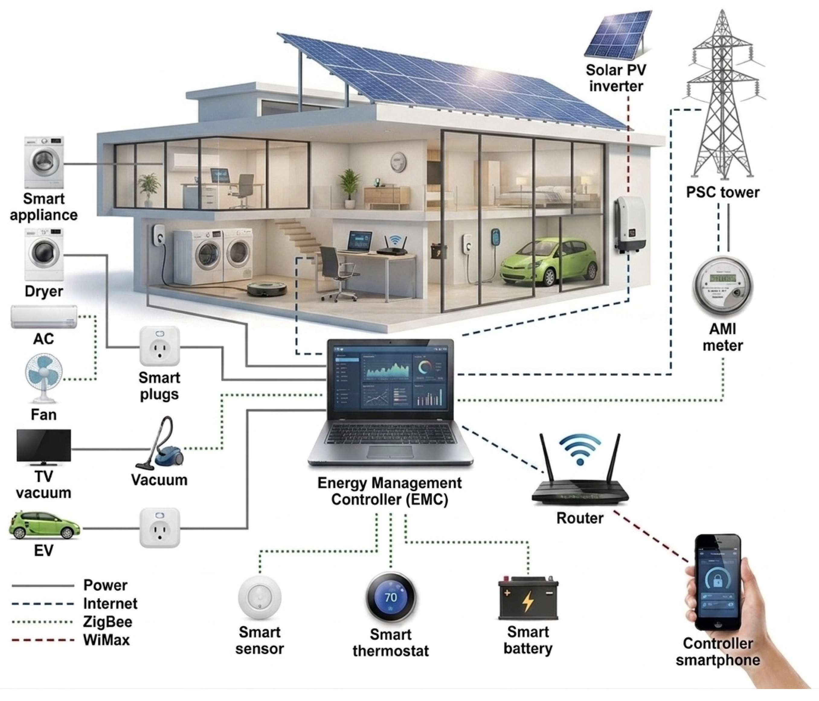
Figure 1 summarizes a Smart Home architecture based on IoT appliances. While this figure demonstrates the physical and communicational infrastructure, the specific intent of this manuscript is to address the underlying algorithmic orchestration required to make this architecture efficient. Coordinating the operational times of these appliances, called the Appliance Energy Scheduling Problem in Smart IoT Home (AESPSH), is mathematically classified as a highly complex, NP-hard multi-objective problem [7,8].

IoT is used to improve general quality of life and comfort in urban areas by linking with smart homes, allowing users to check and run their appliance equipment simply [9,10,11]. A smart home-based IoT system has six core components: smart plugs, an energy management controller, a controller application, smart appliances, communication technologies, and advanced metering (as seen in Figure 1) [6,12,13].

When dealing with Power Supply Planning (PSP), user comfort is a crucial factor [14]. Two main things affect this comfort level: the Waiting Time Rate (WTR) and the Consumed Power Rate (CPR) [15]. The effect of WTR is straightforward: if the delay or waiting time for an appliance increases, user comfort goes down [16]. Regarding CPR, user comfort increases when there is more available power to operate Non-Shiftable Appliances (NSAs) those devices that need to run immediately [17,18].

Various influencing factors are pose complexity to optimization, such as stochastic user behavior, fluctuating tariffs, rigid comfort demands, and IoT network limitations [19,20,21]. Therefore, traditional methods like linear programming and standard metaheuristics frequently suffer from slow convergence and entrapment in local optima and consistently suffer from this variable landscape [22,23].

The primary goal in this study is to address the limitations of the existing scheduling methods based on metaheuristic algorithms by designing a superior hybrid optimization framework that is capable of escaping local optima and attaining a truer global solution for the problem of AESPSH [24]. To achieve this aim, the research produces the scientific question: How can the herd-based metaheuristic algorithm be structurally optimized and mathematically trade off between global exploration and local exploitation to prevent premature convergence in NP-hard scheduling environments?

Thus, the research provides the following specific research questions:

1. How does the combination of a Lévy Flight (LF) optimizer into diverse multi-subpopulations of the CHIO inspire convergence speed and solution accuracy?

2. Which hybridization model achieves the optimal trade-off between grid efficiency, such as EB and PAR minimization, and user comfort parameters like WR and ELR measurements in a smart IoT home?

This study aims mainly to design, implement, and thoroughly evaluate three different hybrid models of the CHIO optimizer that use Lévy Flights (CHIOLF) to optimally schedule smart IoT appliances, thereby minimizing operational costs and peak demand while strictly adhering to user comfort constraints.

Strategically, this study integrates the herd immunity concept of CHIO with Lévy-based exploration. We conduct three structural variations: the LF operator combined with the infected, susceptible, and immune subpopulations of the CHIO algorithm, respectively. The AESPSH optimization framework was utilized as a design tool and integrated evaluation criteria such as economic variables (WR and ELR) and operational criteria (EB, PAR).

To answer the study research question, the experimental results definitively identify the CHIOLF-2 model (where LF is injected into the susceptible subpopulation) as the superior architecture, whereas the CHIOLF-2 hybridized model balances global exploration and local exploitation successfully, with results that show its fastest convergence speed, maximum cost reduction, optimal peak load clipping, and highest user comfort satisfaction against competitor metaheuristic methods in the literature.

To immediately address the recognized energy scheduling problems, this study produces the following contributions:

1. We integrate Lévy Flight to power broader state-space exploration and avoid the CHIO stagnation issue by engineering the CHIOLF algorithm, guaranteeing high solution precision and preventing entrapment in local optima to enhance algorithmic performance and prevent premature convergence. 2. We design and evaluate multi-hybrid models that manipulate different mathematical phases of the CHIO algorithm. This produces a typical approach capable of obtaining an accurate trade-off between conflicting smart home objectives based on variation in grid conditions in targeting subpopulation optimization strategies. 3. We conduct a comprehensive tested scheduling framework (using the superior CHIOLF-2 model) which directly addresses the AESPSH problem conflict by minimizing WR and ELR alongside EB and PAR without violating underlying device health or user comfort constraints by attaining a resolution of conflicting scheduling constraints.

The remaining sections of this article are structured as follows: Section 2 critically reviews the existing metaheuristic methods to AESPSH. This section sets the baseline constraints (slow convergence, local optima) that the study’s question addresses and presents a hybrid approach. Section 3 presents the mathematical framework of the three hybrid methods discussed. It immediately answers the paper’s question concerning how Lévy Flight combination influences subpopulation phases, supporting the theoretical mechanics of our solution. Section 4 summarizes the enforcement of the hybrid models to the real-world engineering problem. Hence, it determines the design tools, operational constraints, and objective functions (EB, PAR, WR, ELR) required to test the stated objectives.

2. Related Works

The Appliance Energy Scheduling Problem in Smart IoT Homes (AESPSH) is no longer a traditional, isolated mathematical problem [25,26]. As modern smart grids evolve, developing an optimal scheduler requires a multidisciplinary approach [5,27,28,29]. Consequently, this section reviews the research in the literature by synthesizing the four major scientific fields that underpin this research: Artificial Intelligence and Computational Optimization, Internet of Things (IoT) management, Energy Systems, and Cybersecurity [30,31].

Metaheuristic algorithms are flexibly permit exploration of problem spaces, exploitation of promising regions, and escape from local optima, whereas these advantages attract the research community to use them for solving the AESPSH problem [32,33,34,35]. Standards optimization methods were deployed in early approaches, such as a study conducted by Rahim et al., which implemented a Genetic Algorithm (GA), Ant Colony Optimization (ACO), and Particle Swarm Optimization (PSO) to solve the multi-objective AESPSH scheduling problem. The experimental results demonstrate that GA yielded the most favorable trade-off between cost and user comfort [34,36,37]. Additionally, the work presented by Ullah et al. [38] deployed a hybrid approach for industrial appliance scheduling. This approach combines the Grasshopper Optimization Algorithm (GOA) with the Cuckoo Search Algorithm (CSA) to demonstrate its hybridized efficiency in addressing the AESPSH.

Subsequently, modern studies have switched toward improved, modified, and hybrid algorithms to avoid the premature convergence and stagnation often seen in standard algorithms. For instance, Manoharan et al. [39] introduce an (IHTBZOA)framework to achieve superior continuous-to-binary mapping for demand response programs by integrating an Inverse Hyperbolic Tangent (ArcTanh) transfer function over the modified Zebra Optimization Algorithm, which has proven exceptionally effective. On the other hand, the study produced by Hafeez et al. [40] outperformed independent GA, PSO, and WDO methods, which depend on the Genetic Wind-Driven Optimization (GWDO) framework. Moreover, a superior Peak-to-Average Ratio (PAR) reduction is achieved by hybridizing the GWD algorithm by Javaid et al. [41]. Meanwhile, a study by Ahmad et al. [42] significantly reduced electricity bills (EB) based on integrating GA with PSO (HGPO) model. Furthermore, attaining superior EB and PAR reductions, albeit with minor compromises to user comfort compared with standard GA, was achieved by the work produced by Qureshi et al. [43], which combined WDO, the Harmony Search Algorithm (HSA), and Evolutionary Differential Equations into EDHWDO. These advancements in hybridization strongly justify the development of the Coronavirus Herd Immunity Optimizer–Lévy Flight (CHIOLF) algorithm proposed in this study.

The implementation of AI-driven scheduling decisions that relies on robust IoT infrastructure advances the connection, management, and orchestration of various smart home appliances. Several kinds of IoT ecosystems are modeled in the literature, with growing complexity. For example, single and multiple interconnected smart homes are distributed and implemented by Javaid et al. [41] to test their optimization models on complex datasets encompassing up to 12 appliances. Recently, the next trend of research has focused heavily on the dynamic management of residential microgrids via IoT ecosystems. According to Ren et al. [44], it jointly manages residential appliance scheduling alongside Battery Energy Storage System (BESS) capacity within photovoltaic networks to overcome the AESPSH using a two-stage optimization approach. Likewise, a study that optimizes cost efficiency and user satisfaction while maintaining the physical durability of storage devices for Smart Home Energy Management Systems (SHEMS) depends on developed comprehensive static and dynamic models. Their framework specifically leverages IoT data to incorporate uncertainty via scenario analysis [45].

A dynamic pricing scheme is a critical facet of AESPSH; it involves seamless integration with macro-level Energy Systems, while ensuring the scheduling algorithms simultaneously minimize user costs, overall consumption, and grid peak loads. Work conducted by Zhao et al. [46] utilizes GA with constraints to merge Real-Time Pricing (RTP) and Inclining Block Rate (IBR) schemes, aiming to balance energy consumption over a specified horizon. Other studies [47] successfully utilized Time-of-Use (TOU) pricing to minimize costs.

Complex renewable energy trading and strict environmental constraints are increasingly integrated into the scheduling matrix in contemporary research. A multi-objective framework that deployed a Marine Predators Algorithm (MPA) for renewable energy trading is proposed by Kumar et al. [48]. This study moved beyond conventional revenue-only strategies to integrate photovoltaic systems, wind turbines, EVs, and BESS with carbon awareness under day-ahead RTP. Extending the scope of objective criteria, a study introduced by Firouzabad et al. [49] plays a vital role in residential scheduling by optimizing global energy consumption when it utilizes the NSGA-II method to manage six distinct objectives—including electricity cost, total energy consumption, peak demand, thermal indices, and CO2 emissions, respectively.

In conclusion, while diverse methods have enhanced the singular fields of optimization, IoT management, and energy grid integration, there remains a crucial requirement for highly robust hybrid algorithms capable of navigating this multidisciplinary complexity. These works have highlighted a gap for scheduling models that can definitively prevent premature algorithmic convergence while strictly adhering to grid constraints, economic variables, and user comfort. The proposed hybrid CHIOLF addresses this specific gap.

3. Hybridized Coronavirus Herd Immunity Optimizer with Lévy Flight Models for Appliances Energy Scheduling Problem in Smart IoT Homes

Empirically, the CHIO algorithm is used in a vast area of optimization scopes due to its efficient and powerful mechanism to tackle several optimization problems [24]. In the CHIO algorithm, two strategies are mimicked and modeled, namely herd immunity and social distancing for optimization concepts. The CHIO population is organized by three types of community-based individuals, such as infected, susceptible, and immunized, that are utilized for herd immunity. This population distribution is used to define how the modern-initiated solution updates its genes with social distancing strategies. The forthcoming sentences explain in detail the evolutionary mechanism of the CHIO algorithm to update its different communities at each population, and how many generations are conducted in the searching process to locate an approximate-optimal solution to the target optimization problem [27]. Furthermore, demonstrate how the hybridization of CHIO with LF is established based on the three different hybridization models.

Step 1: Problem Formulation: The problem is formulated, and the CHIO parameters are initialized The optimization problem is stated as an objective function, as illustrated in Equation (1):

$$minf\left(x\right)x\in [lb,ub]$$

(1)

where f(x) is the calculated individual’s measurable objective function, $x_i=(x_1,x_2,\dots ,x_n)$, where n is the number of genes in each individual and $x_i$ is the gene indicated by the symbol i. Each gene’s value range is xi [lbi, ubi], where lbi and ubi are the gene xi’s lowest and highest bounds, respectively. The CHIO method evolves four algorithmic parameters and two operational parameters: HIS, C0, n, and Max_Itr. Two key control parameters are generated: the basic reproduction rate (BRr) describing the propagation of the coronavirus between people, and the maximum age of infected cases (Max_Age) for defining recovery or death. These parameters are critical for enabling CHIO to effectively detect and monitor the spread of coronavirus through people [24].

Step 2: Create a population with herd immunity, The CHIO generates a population with herd immunity by randomly creating a set of cases (individuals) and keeping them in the herd immunity population (HIP) as a two-dimensional matrix. Each case’s objective function (immunity rate) is calculated using Equation (2). A susceptible or infected case creates a status vector (S) of length HIS for all HIP cases, randomly starting with C0 infected cases in the population.

$$\begin{array}{cc}\hfill \mathit{HIP}=& \left[\begin{array}{cccc}e{s}_1^1& e{s}_2^1& \dots & e{s}_m^1\\ e{s}_1^2& e{s}_2^2& \dots & e{s}_m^2\\ ⋮& ⋮& \dots & ⋮\\ e{s}_1^n& e{s}_2^n& \dots & e{s}_m^n\end{array}\right],\end{array}$$

(2)

Step 3: Evolution of hybrid coronavirus herd immunity with Lévy Flight, In the CHIO algorithm, evolution is the main CHIO loop for advancement. Three rules based on BRr determine whether gene $\left(e{s}_i^j\right)$ of instance $\left(e{s}^j\right)$ remains same or is influenced by social distance:

$$e{s}_i^j(t+1)=\left\{\begin{array}{cc}e{s}_i^j\left(t\right),\hfill & r\ge B{R}_r,\hfill \\ C\left(x_i^j\left(t\right)\right),\hfill & r<{\displaystyle \frac{1}{3}}B{R}_r\left(\mathrm{infected}\right),\hfill \\ N\left(x_i^j\left(t\right)\right),\hfill & r<{\displaystyle \frac{2}{3}}B{R}_r\left(\mathrm{susceptible}\right),\hfill \\ R\left(x_i^j\left(t\right)\right),\hfill & r<B{R}_r\left(\mathrm{immuned}\right)\hfill \end{array}\right.$$

(3)

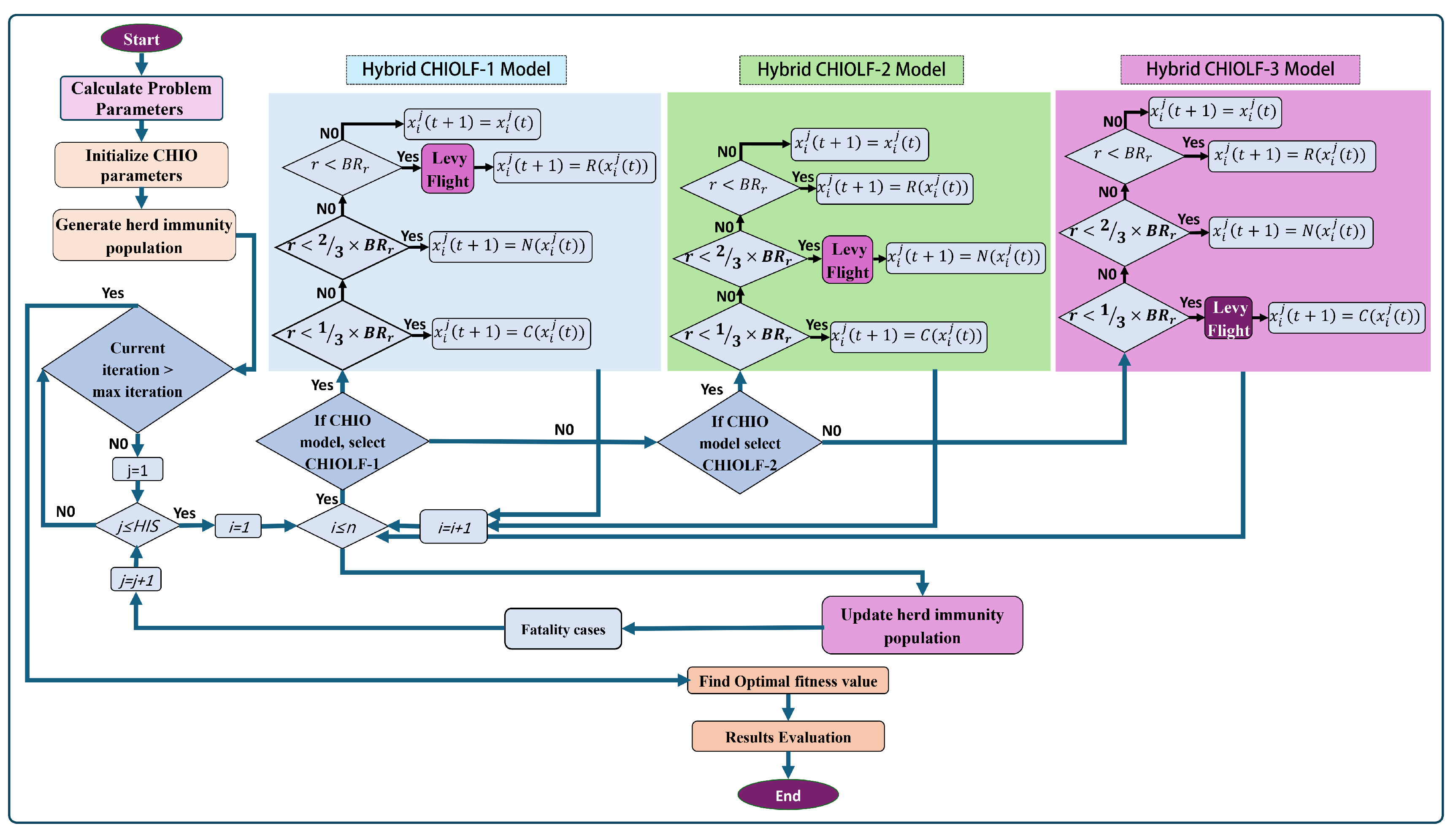
where r is a random number in [0, 1]. These rules will be discussed in the following order to explain how the three hybridized models were conducted, as we show in Figure 2: Infected community(subpopulation): individuals in the inferior (infected) subpopulation value range $r\in [0,1/3BRr]$, the mechanism of generating a new individual (candidate solution) of the hybrid CHIOLF-1 according to Equation (3) from the infected community (subpopulation) will be modified using Lévy Flight, and the new solution can be defined as:

In the proposed hybrid CHIOLF-1 approach, the new solution generation mechanism is modified by integrating a Lévy Flight into the infected case updating process. The updated equation is formulated as in Equation (4):

$$e{s}_i^j(t+1)=\left\{\begin{array}{cc}C\left(e{s}_i^j\left(t\right)\right)+\alpha \otimes \mathrm{L}é\mathrm{vy}\left(\beta \right),\hfill & r<{\displaystyle \frac{1}{3}}B{R}_r\hfill \end{array}\right.$$

(4)

where:

• $\alpha$ is the Lévy step size scaling factor;
• ⊗ denotes element-wise multiplication;
• $\mathrm{L}é\mathrm{vy}\left(\beta \right)$ is the random step generated according to the Lévy probability distribution;
• $\beta$ is the Lévy distribution parameter.

The Lévy Flight step is mathematically generated based on [31,50]:

$$\mathrm{L}é\mathrm{vy}\left(\beta \right)={\displaystyle \frac{u}{{\left|v\right|}^{1/\beta }}}$$

(5)

where:

$$u\sim N(0,{\sigma }_u^2),v\sim N(0,{\sigma }_v^2)$$

(6)

and:

$${\sigma }_u={\left[{\displaystyle \frac{\Gamma (1+\beta )sin(\pi \beta /2)}{\Gamma ((1+\beta )/2)\beta 2^{(\beta -1)/2}}}\right]}^{1/\beta }$$

(7)

$${\sigma }_v=1$$

(8)

Susceptible community: Candidate solutions (individuals) at the susceptible subpopulation value range $r\in [1/3BRr,2/3BRr]$; according to Equation (3), the mechanism of generating a solution of the CHIOLF-2 model for the susceptible cases will be modified using Lévy Flight, and the new solution can be defined as:

In the proposed hybrid CHIOLF-2 approach, the new solution generation mechanism is modified by integrating a Lévy flight into the susceptible case updating process. The updated equation is formulated as in Equation (9):

$$e{s}_i^j(t+1)=\left\{\begin{array}{cc}N\left(e{s}_i^j\left(t\right)\right)+\alpha \otimes \mathrm{L}é\mathrm{vy}\left(\beta \right),\hfill & r<{\displaystyle \frac{2}{3}}B{R}_r\hfill \end{array}\right.$$

(9)

Immune community: At the superior (immune) subpopulation, individuals’ value range $r\in [2/3BRr,BRr]$; the new solution is updated by integrating a Lévy Flight into the immune case for the hybrid CHIOLF-3 model. The updated equation is formulated as in Equation (10):

$$e{s}_i^j(t+1)=\left\{\begin{array}{cc}R\left(e{s}_i^j\left(t\right)\right)+\alpha \otimes \mathrm{L}é\mathrm{vy}\left(\beta \right),\hfill & r<B{R}_r\hfill \end{array}\right.$$

(10)

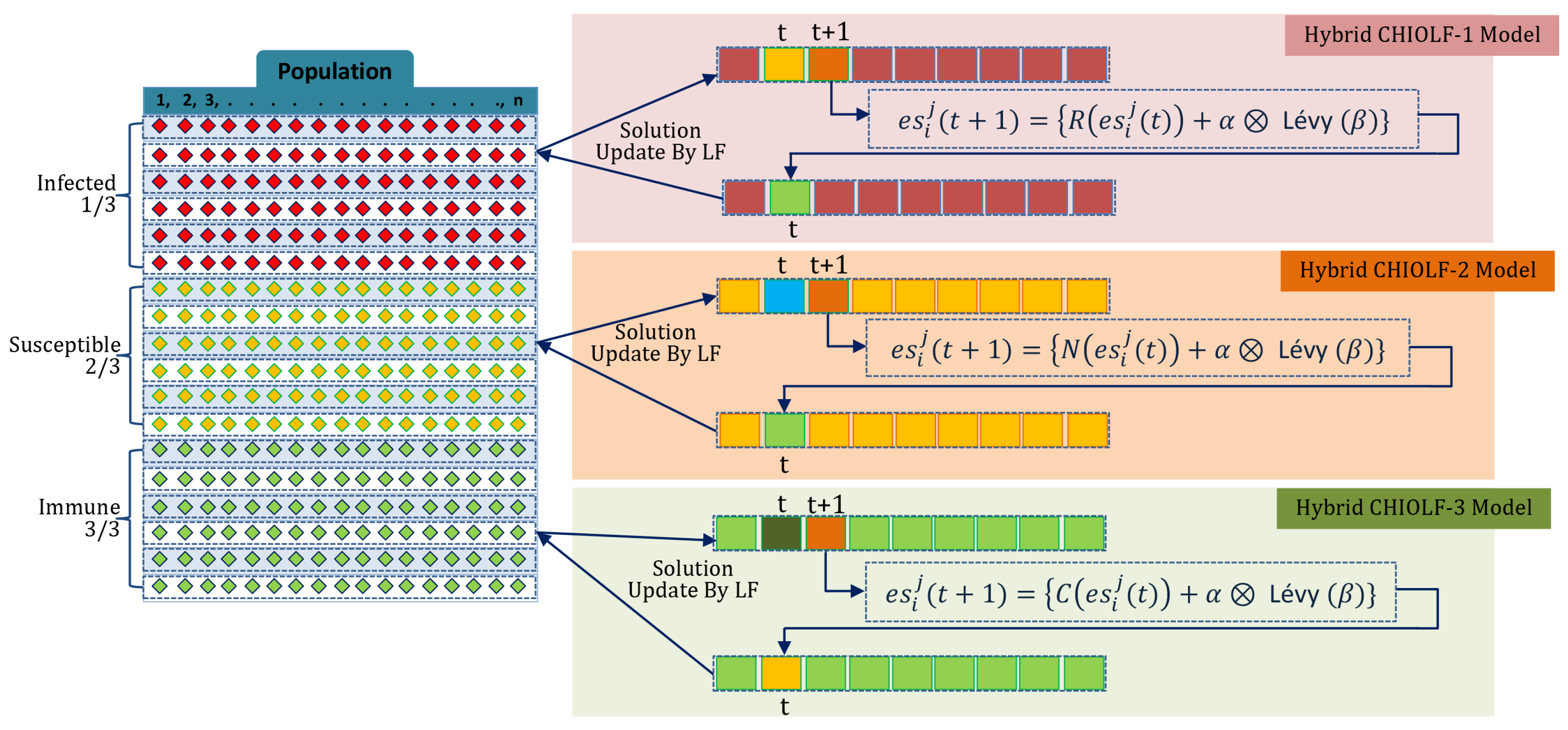
Figure 3 shows different updating solution strategies (solution representation) of the produced different hybrid CHIOLF-1, CHIOLF-2, and CHIOLF-3 models. Specifically, Firstly explains how the proposed CHIOLF-1 hybridization mechanism significantly enhances the exploration capability of CHIO. Whereas the short steps generated by the Lévy distribution operator will enhance global exploration to find a new region in the search area to avoid inferior (infected) individuals in the infected subpopulation. Secondly, the Lévy distribution operator robustifies the exploration capability of the CHIO algorithm by improving the susceptibility of individuals to find promising solutions to wellness at the proposed CHIOLF-2 model and can balance exploration and exploitation search mechanisms. Finally, presents how the proposed CHIOLF-3 hybridization mechanism significantly improves the exploitation capability of CHIO. Specifically, the short steps generated by the Lévy distribution enhance local exploitation around promising regions, while occasional long jumps enable the search agents to escape local minima and investigate unexplored areas of the search space.

Step 4: Population Update, the immunity rate is calculated for each created case, and the generated person replaces the current solution if $f\left(e{s}_j(t+1)\right)<f\left(e{s}_j\left(t\right)\right)$. If the status vector $e{s}_j$ has a value of 1, the age vector $\left(A_j\right)$ is increased by 1.

Step 5: Fatal cases, if the immunity rate cannot increase for the number of iterations indicated by $Ma{x}_{A}ge$, the infected case ($Sj=1$) is said to have died. The case can be recreated from scratch using $e{s}_i^j=l{b}_i+(u{b}_i-l{b}_i)\in (0,1)$, $\forall i=1,2,...,n,$ with $A_j$ and $S_j$ set to zero. Diversifying the population can avoid local optima.

Step 6: Stopping condition, the CHIOLF iterates via Steps 3–5 until it meets the stopping criteria, which is based on the maximum number of iterations. In this instance, the population is mainly composed of susceptible and immune individuals, and the affected instances disappear.

3.1. Formulation of the Appliance Energy Scheduling Problem in Smart IoT Home

In this section, we present the theoretical framework of the AESPSH problem as a multi-objective optimization for scheduling operational times of smart IoT appliances. The formulation encompasses all objectives of AESP, encompassing electricity cost (EC), Peak-to-average ratio (PAR), and user comfort (UC) level.

3.1.1. Classification of Smart Appliances

In accordance with the categorization approach observed in prior studies [18,37,41,47], this study classifies smart home appliances into two main kinds depending on their operations: Shiftable Appliances (SA) and Non-Shiftable Appliances (NSA). The SA group comprises appliances that work automatically, while the NSA class encompasses appliances that require manual operation. The illustration and formulation of these classes are presented below:

• Shiftable Appliances The SAs are designed to operate automatically. Users have the flexibility to predefine both the allowable periods for operation ($APO$) and the cycle length required to complete their tasks ($CLO$). For instance, users can set $APO$ and $CLO$ parameters to initiate the operation of appliances such as a washing machine or clothes dryer at predetermined times in advance.
  The SAs are represented as a vector S as follows:

  $$S=[s_1,s_2,\dots ,s_m],$$

  (11)

  where $s_i$ is the SA i, m denotes the total number of SAs. The SAs can be organized to operate at a time horizon (T). The time horizon T is split into 1440 time slots (Equation (12)).

  $$T=[t^1,t^2,\dots ,t^{1}440],$$

  (12)

  where $t^j$ is a time slot j. The SA’s energy required to complete its operation task is expressed as follows:

  $$\begin{array}{cc}\hfill \mathit{ES}=& \left[\begin{array}{cccc}e{s}_1^1& e{s}_2^1& \dots & e{s}_m^1\\ e{s}_1^2& e{s}_2^2& \dots & e{s}_m^2\\ ⋮& ⋮& \dots & ⋮\\ e{s}_1^n& e{s}_2^n& \dots & e{s}_m^n\end{array}\right],\end{array}$$

  (13)

  where $p{s}_i^j$ is the energy required by $s_i$ to be operated, and n is the total number of time slots, which is 1440. As discussed earlier, the SA’s time parameters, including $APO$ and $CLO$, need to be predefined by users. The $APO$ consists of the beginning operation period, denoted as $AP{O}_s$, and the ending operation period, denoted as $AP{O}_e$, as follows:

  $$AP{O}_s=[AP{O}_{s1},AP{O}_{s2},\dots ,AP{O}_{sm}],$$

  (14)

  $$AP{O}_e=[AP{O}_{e1},AP{O}_{e2},\dots ,AP{O}_{em}],$$

  (15)
  The notation $AP{O}_{si}$ and $AP{O}_{ei}$ refer to the starting and ending allowable periods for the scheduling and operation of $s_i$.
  The $CLO$ is shown as a vector:

  $$CLO=[c_1,c_2,\dots ,c_m],$$

  (16)

  where $c_i$ denotes the $CLO$ of $s_i$. The SAs should be operated at a specific time. The starting and ending times are presented as follows:

  $$So=[s{o}_1,s{o}_2,\dots ,s{o}_m],$$

  (17)

  $$Eo=[e{o}_1,e{o}_2,\dots ,e{o}_m],$$

  (18)

  where $So$ and $Eo$ are the starting and ending times of SAs’ operations, respectively.
• Non-shiftable Appliances NSAs are run manually, and users cannot define their time parameters, such as $APO$ and $CLO$, in advance. Examples of such appliances include TVs and computer chargers, where users do not have the capability to predefine the $APO$ and $CLO$ ahead of time.
  NSAs are given in a vector named $NS$:

  $$NS=[n{s}_1,n{s}_2,\dots ,n{s}_q],$$

  (19)

  where $n{s}_k$ denotes the NSA k, q is the total number of NSAs. The energy needed by each NSA is denoted as $ENS$ and formulated as follows:

  $$ENS=[en{s}_1,en{s}_2,\dots ,en{s}_q],$$

  (20)

  where $en{s}_k$ denotes the energy required by $n{s}_k$.

3.1.2. Electricity Bill

EB minimization stands out as a primary objective in addressing the AESP, given its significance in incentivizing households to reschedule the operations of their appliances. The calculation of EB can be expressed as follows:

$$EB={\displaystyle \sum _{j=1}^n}{\displaystyle \sum _{i=1}^m}e{s}_i^j\times tr{f}^j,$$

(21)

where $tr{f}^j$ denotes the tariff of electricity at time slot j that is extracted from the dynamic pricing scheme. The dynamic pricing adopted in this research is the RTP, chosen for its user-friendly flexibility. The RTP scheme entails hourly price adjustments based on the current energy generation cost. Additionally, RTP is synergistically combined with an IBR due to its efficacy in balancing and smoothing energy demand throughout T [1,25,26,35]. The IBR scheme sets only two tariffs based on the amount of energy consumed, and it is expressed as follows:

$$tr{f}^j=\left\{\begin{array}{cc}{l}^j\hfill & \mathrm{if}0\le tr{f}^j\le Th\hfill \\ h^j\hfill & \mathrm{if}tr{f}^j>Th\hfill \end{array}\right.,$$

(22)

$$h^j=\lambda \times l^j,$$

(23)

where $l^j$ and $h^j$ denote the low and high tariffs, respectively, $Th$ represents the energy consumed threshold, and $\lambda$ is a positive number.

3.1.3. Peak-to-Average Ratio

The PAR signifies the ratio between the highest and average consumption within T. Minimizing PAR is crucial for improving the energy system of SGs as it contributes to balancing and reducing energy requests during peak periods. The formulation of PAR is presented in Equation (24).

$$PAR={\displaystyle \frac{E{S}_{max}}{E{S}_{Avg}}},$$

(24)

where

$$E{S}_{Avg}={\displaystyle \frac{{\sum }_{j=1}^{n}e{s}^j}{n}},$$

(25)

$E{S}_{max}$ and $E{S}_{avg}$ are the highest and average energy consumed.

3.1.4. User Comfort

The UC level can be improved and maintained through two contributing factors: the Waiting Rate ($WR$) and the Energy Limit Rate ($ELR$). The $WR$ improves the UC level by minimizing the waiting time for operating SAs, while the $ELR$ is utilized to enhance UC by allowing the operation of more NSAs without surpassing a predefined threshold $Th$ [35].

The $WR$ of i is computed as follows:

$$W{R}_i={\displaystyle \frac{s{o}_i-APO{s}_i}{APO{e}_i-APO{s}_i-c_i}},\forall i\in \mathit{S},$$

(26)

The average $WR$ can be calculated using Equation (27).

$$W{R}_{avg}={\displaystyle \frac{{\sum }_{i=1}^m(s{o}_i-APO{s}_i)}{{\sum }_{i=1}^m(APO{e}_i-APO{s}_i-c_i)}},$$

(27)

$ELR$ at a specific time slot is calculated as follows:

$$EL{R}^j={\displaystyle \frac{{\sum }_{k=1}^{q}ON{A}_k^j}{q}},$$

(28)

${\sum }_{k=1}^{q}ON{A}_k^j$ is the number of $NSAs$ that consumed more energy the $Th$, and can be calculated as follows:

$$ON{A}_k^j=\left\{\begin{array}{cc}0\hfill & \mathrm{if}EN{S}_k<A{E}^j\hfill \\ 1\hfill & otherwise,\hfill \end{array}\right.,$$

(29)

$$A{E}^j=Th-{ES}^j,$$

(30)

$A{E}^j$ is the available energy to operate the NSAs. The $ELR$ average value is computed as follows:

$$EL{R}_{avg}={\displaystyle \frac{{\sum }_{j=1}^n{\sum }_{k=1}^{q}ON{A}_k^j}{q\times n}},$$

(31)

$$UC=\left(1-\left({\displaystyle \frac{W{R}_{avg}+EL{R}_{avg}}{2}}\right)\right)\times 100\%,$$

(32)

3.1.5. Multi-Objective Optimization of Appliances Energy Scheduling Problem in Smart IoT Home

The AESPSH in this study is formulated as a multi-objective optimization problem, aiming to jointly optimize multiple objectives, including EB, PAR, WR, and ELR. For the optimization of AESPSH, a non-Pareto scalarization method known as the weighted sum method is employed. This method is selected for its simplicity, ease of implementation, lack of complexity, and widespread use in state-of-the-art AESPSH methods [28,29,30,32,33].

In this formulation, the concept of Pareto optimality is disregarded due to its inefficiency in handling optimization problems with multiple objectives, as is the case with AESPSH [34,36,51]. The multi-objective function of AESPSH is structured as follows:

$$\begin{array}{c}\hfill minF\left(X\right)=w_1\times {\displaystyle \frac{EB}{EB+A}}+w_2\times {\displaystyle \frac{PAR}{PAR+B}}+w_3\times W{R}_{avg}+w_4\times EL{R}_{avg}\end{array},$$

(33)

where A and B are two positive numbers, and $w_1,w_2,w_3,$ and $w_4$ showing significance of the objectives.

4. Experimental Results of the Coronavirus Herd Immunity Optimizer with Lévy Flight Models in Appliances Energy Scheduling Problem in Smart IoT Home

In this section, we provide a clear demonstration of the results evaluation for the proposed hybrid CHIOLFs models from one side to determine which model has superiority over others. On the second side, we compare the best CHIOLF model against competitor algorithms in the literature based on the AESPSH problem. All comparisons were conducted using seven consumption scenarios and four evaluation metrics, such as EB cost reduction, PAR minimization, and maximization of the user leisure level, which include (WR and ELR) criteria.

4.1. Experimental Design of Appliances Energy Scheduling Problem in Smart IoT Home Settings

As we mentioned before, seven different consumption scenarios are used to evaluate the seven scenarios separately chosen in this study, and the proposed CHIOLFs methods are tested. Additionally, this study employs a dynamic pricing scheme that combines WR and ELR metrics. The Commonwealth Edison Company is the source of the WR scheme that was registered from 1st to 7th of June 2016 (7 days), while $\lambda$ and C are set to be 1.543 and 0.0333 per time slot that the ELR scheme uses, respectively (Equation (22)) [25,46].

Table 1. Main characteristics of the appliance time parameters.

NO.	Appliances	LOC	OTPs–OTPe	NO.	Appliances	LOC	OTPs–OTPe
1	Dishwasher	105	540–780	19	Dehumidifier	30	1–120
2	Dishwasher	105	840–1080	20	Dehumidifier	30	120–240
3	Dishwasher	105	1200–1440	21	Dehumidifier	30	240–360
4	Air Conditioner	30	1–120	22	Dehumidifier	30	360–480
5	Air Conditioner	30	120–240	23	Dehumidifier	30	480–600
6	Air Conditioner	30	240–360	24	Dehumidifier	30	600–720
7	Air Conditioner	30	360–480	25	Dehumidifier	30	720–840
8	Air Conditioner	30	480–600	26	Dehumidifier	30	840–960
9	Air Conditioner	30	600–720	27	Dehumidifier	30	960–1080
10	Air Conditioner	30	720–840	28	Dehumidifier	30	1080–1200
11	Air Conditioner	30	840–960	29	Dehumidifier	30	1200–1320
12	Air Conditioner	30	960–1080	30	Dehumidifier	30	1320–1440
13	Air Conditioner	30	1080–1200	31	Electric Water Heater	35	300–420
14	Air Conditioner	30	1200–1320	32	Electric Water Heater	35	1100–1440
15	Air Conditioner	30	1320–1440	33	Coffee Maker	10	300–450
16	Washing Machine	55	60–300	34	Coffee Maker	10	1020–1140
17	Clothes Dryer	60	300–480	35	Robotic Pool Filter	180	1–540
18	Refrigerator	1440	1–1440	36	Robotic Pool Filter	180	900–1440

and

Table 2. NSAs used in the Time scheduling.

No.	Appliances	Power (kW)
1	Light [47]	0.6
2	Attic Fan [53]	0.3
3	Table Fan [53]	0.8
4	Iron [47]	1.5
5	Toaster [53]	1
6	Computer Charger [53]	1.5
7	Cleaner [46]	1.5
8	TV [53]	0.3
9	Hair Dryer [53]	1.2
10	Hand Drill [53]	0.6
11	Water Pump [53]	2.5
12	Blender [53]	0.3
13	Microwave [47]	1.18
14	Electric Vehicle [54]	1

present the key parameters and features of smart home appliances that were utilized in this study (i.e., SAs and NSAs). These data were not generated experimentally but collected from previously published works in the literature, which are widely used benchmarks in the AESPSH domain and report complete, peer-reviewed appliance specifications [52]. The values were transcribed into [MS Excel 2026/MATLAB R2025b], verified against the original sources, and standardized to consistent units before being organized into the tables, with the source indicated in each table caption. Each of the seven scenarios used up to thirty-six SAs and 14 NSAs, as shown in

Table 3. Main characteristics of the seven tested scenarios.

Sens	Appliances
Sen #1	1, 3, 4, 5, 6, 7, 15, 18, 19, 20, 21, 22, 23, 24, 25, 26, 27, 28, 29, 30, 31, 33, 35
Sen #2	1, 2, 4, 5, 6, 7, 10, 11, 12, 18, 25, 26, 27, 28, 29, 31, 32, 33, 34, 36
Sen #3	3, 4, 5, 6, 7, 8, 9, 10, 11, 12, 13, 14, 15, 18, 23, 24, 25, 26, 27, 28, 31, 32, 33, 34, 35
Sen #4	1, 2, 3, 4, 5, 6, 7, 8, 9, 10, 11, 12, 13, 14, 15, 16, 17, 18, 19, 20, 21, 22, 23, 24, 25, 26, 27, 28, 29, 30, 31, 32, 33, 34, 35, 36
Sen #5	3, 4, 5, 6, 7, 8, 9, 10, 11, 12, 13, 14, 15, 18, 23, 24, 25, 26, 27, 28, 31, 32, 33, 34, 35
Sen #6	1, 2, 3, 8, 9, 10, 11, 12, 18, 19, 20, 21, 22, 23, 24, 25, 26, 27, 28, 29, 30, 31, 33, 34, 35
Sen #7	1, 3, 4, 5, 6, 7, 8, 9, 10, 11, 12, 13, 14, 15, 16, 17, 18, 19, 20, 21, 22, 23, 24, 25, 26, 27, 28, 29, 30, 31, 33, 34, 35, 36

, where the scenario’s column represents the scenario number, and the appliances’ column denotes the appliance number mentioned in Table 1.

For each scenario and algorithm, 30 independent runs are tested to ensure fair results and comparisons concerning multi-objective optimization with predefined stopping criteria and parameter settings. At each run, the algorithms perform 1000 iterations, as 1000 generations are sufficient for convergence [55].

Table 4. Parameters of Coronavirus Herd Immunity Optimizer algorithm.

Parameter	Value
Population Size ($HIS$)	40
Max Iteration (I)	1000

lists CHIO parameter settings that include population size (HIS) and max iterations (I), while other parameters, such as $R{B}_r$ and $Ma{x}_{Age}$, are not mentioned because their values are tuned to get their best values.

4.2. Analysis of Coronavirus Herd Immunity Optimizer with Lévy Flight Parameters

As we mentioned before, the CHIOLF algorithm has two control parameters, including $R{B}_r$ and $Ma{x}_{Age}$, which affect the CHIO’s sensitivity. Therefore, the $R{B}_r$ and $Ma{x}_{Age}$ parameters are investigated and analyzed to get their best values to achieve optimal schedules in the proposed CHIOLF.

Four values in both of the $R{B}_r$ and $Ma{x}_{Age}$ are studied to demonstrate their effectiveness; these values are such as 0.005, 0.05, 0.1, and 0.5 for $R{B}_r$ and 50, 100, 300, and 500 for $Ma{x}_{Age}$, respectively [24]. Multi-objective in the AESPSH problem, such as EB, PAR, WR, and ELR, are applied to evaluate the value of the control parameters, as we show in

Table 5. Coronavirus Herd Immunity Optimizer Parameters Analysis.

		0.005				0.05				0.1				0.5
	Sens	EB	PAR	WR	ELR	EB	PAR	WR	ELR	EB	PAR	WR	ELR	EB	PAR	WR	ELR
50	Sen #1	43.4641	2.6807	0.2242	0.3227	43.8147	2.6044	0.0094	0.3127	43.7384	2.6045	0.0087	0.3129	43.5523	2.6045	0.0458	0.3164
	Sen #2	64.1402	2.6446	0.2086	0.3462	64.6208	2.4323	0.0124	0.3453	64.4169	2.4254	0.0147	0.3455	64.2613	2.4169	0.0297	0.3460
	Sen #3	65.9196	2.3865	0.2182	0.3934	66.4258	2.2181	0.0150	0.3803	66.3190	2.2117	0.0144	0.3805	66.3121	2.2225	0.0405	0.3832
	Sen #4	63.2499	2.5270	0.2356	0.5101	63.3545	1.8744	0.0431	0.5066	63.3702	1.9665	0.0388	0.5096	62.8679	2.0783	0.0838	0.5135
	Sen #5	46.5781	2.4151	0.2125	0.3929	46.7815	2.2203	0.0157	0.3806	46.7853	2.2160	0.0124	0.3801	46.6086	2.2139	0.0423	0.3843
	Sen #6	52.4087	2.5095	0.2031	0.3570	52.6468	2.5175	0.0095	0.3490	52.4176	2.5040	0.0143	0.3500	52.2710	2.5060	0.0388	0.3521
	Sen #7	63.3368	2.3054	0.2535	0.4800	63.0784	2.004	0.0386	0.4661	63.2179	2.0385	0.0337	0.4656	62.9447	2.0086	0.0763	0.4729
100	Sen #1	43.5971	2.7084	0.2041	0.3220	43.8176	2.6044	0.0076	0.3122	43.8085	2.6045	0.0089	0.3128	43.4891	2.6024	0.0379	0.3164
	Sen #2	63.4767	2.5924	0.2266	0.3489	64.4900	2.4248	0.0136	0.3454	64.290	2.4199	0.0123	0.3456	64.5717	2.4332	0.0304	0.3460
	Sen #3	66.4986	2.3235	0.2269	0.3931	66.6698	2.2246	0.0123	0.3791	66.4452	2.216	0.0138	0.3801	66.0401	2.2203	0.0408	0.3844
	Sen #4	62.8937	2.4846	0.2365	0.5113	63.3123	1.9471	0.0373	0.5104	63.2181	1.9723	0.0388	0.5104	62.7356	2.0188	0.0875	0.5157
	Sen #5	46.4773	2.4009	0.2209	0.3931	46.7609	2.2160	0.0154	0.3802	46.4528	2.2117	0.0190	0.3817	46.7672	2.2273	0.0456	0.3841
	Sen #6	51.9756	2.5213	0.2208	0.3608	52.5642	2.5175	0.0116	0.3491	52.1948	2.4944	0.0153	0.3508	52.2699	2.5060	0.0326	0.3515
	Sen #7	63.1163	2.3252	0.2346	0.4784	63.3557	2.0195	0.0297	0.4643	63.0719	2.0152	0.0362	0.4661	62.8943	2.0117	0.0723	0.4724
300	Sen #1	43.5265	2.6543	0.2239	0.3224	43.8004	2.6044	0.0074	0.3126	43.8163	2.6045	0.006	0.3123	43.6746	2.6024	0.0352	0.3156
	Sen #2	64.3299	2.5915	0.2181	0.3473	64.4096	2.4244	0.0112	0.3454	64.2427	2.4199	0.0129	0.3456	64.4953	2.4341	0.026	0.3459
	Sen #3	66.0201	2.3541	0.2266	0.3944	66.7045	2.2267	0.0102	0.3790	66.6802	2.2246	0.0102	0.3791	66.3345	2.2246	0.0425	0.3838
	Sen #4	63.1029	2.4434	0.2352	0.5131	63.0111	1.9239	0.0386	0.5118	63.2983	1.9223	0.0404	0.5112	62.5525	2.0766	0.0785	0.5132
	Sen #5	46.3968	2.3109	0.2172	0.3955	46.6641	2.2117	0.0167	0.3804	46.4139	2.2010	0.0159	0.3816	46.4839	2.216	0.0379	0.3847
	Sen #6	52.6838	2.5650	0.1999	0.3565	52.4779	2.5117	0.0102	0.3494	52.1136	2.4887	0.0141	0.3509	52.2548	2.506	0.0295	0.3516
	Sen #7	63.2469	2.4141	0.2121	0.4740	63.2371	2.0133	0.0296	0.4647	63.1973	2.0118	0.0325	0.4653	62.3167	2.0149	0.081	0.4751
500	Sen #1	43.3217	2.603	0.2088	0.3234	43.8209	2.6044	0.0066	0.3123	43.8142	2.6045	0.0059	0.3124	43.6684	2.6024	0.0251	0.315
	Sen #2	64.04	2.6589	0.1998	0.3479	64.6379	2.4359	0.0098	0.3453	64.2235	2.4176	0.0138	0.3456	64.5138	2.4321	0.0284	0.346
	Sen #3	65.9527	2.3322	0.216	0.3919	66.6666	2.2246	0.0107	0.3791	66.642	2.2225	0.0111	0.3795	66.2984	2.223	0.0451	0.3843
	Sen #4	63.6569	2.5122	0.2225	0.5076	63.3165	1.9488	0.0350	0.5097	63.0808	1.9197	0.0373	0.5113	62.8417	1.9618	0.0883	0.5173
	Sen #5	46.5366	2.3837	0.1951	0.3933	46.5411	2.2095	0.0143	0.3808	46.4481	2.2031	0.0149	0.3811	46.3428	2.2165	0.0443	0.3855
	Sen #6	52.532	2.5412	0.1905	0.358	52.0938	2.4944	0.0126	0.3508	52.3337	2.5002	0.0103	0.35	52.4137	2.5156	0.0321	0.3517
	Sen #7	62.9267	2.2803	0.2238	0.4807	63.2214	2.0288	0.0304	0.4647	63.0749	2.0071	0.0337	0.466	62.5727	2.0133	0.0839	0.4755

. The obtained results according to all probable experiments are presented in Table 5 using different possible values of the $RBr$ and $Ma{x}_{Age}$ parameters, where each value of the first parameter is compared with all values of the second parameter.

Based on the results of CHIOLF control parameters presented in Table 5, CHIOLF achieved robust performance six times when the values of the $R{B}_r$ and $Ma{x}_{Age}$ parameters were 0.05 and 50, respectively, which includes two times in the best PAR, one time for best WR, and finally the ELR has three times with best results.

Table 6. Coronavirus Herd Immunity Optimizer’s control parameters for Appliances Energy Scheduling Problem in Smart IoT Home objectives.

Sens	EB	PAR	WR	ELR
Sen #1	0.005/500	0.5/100, 300, 500	0.1/500	0.05/100
Sen #2	0.005/100	0.5/50	0.05/500	0.05/50, 500
Sen #3	0.005/50	0.1/50	0.05, 0.1/300	0.05/300
Sen #4	0.5/300	0.05/50	0.05/500	0.05/50
Sen #5	0.5/500	0.1/300	0.1/50	0.1/50
Sen #6	0.005/100	0.1/300	0.05/50	0.05/50
Sen #7	0.5/300	0.05/50	0.05/300	0.05/100

presents the significant differences between various values of $RBr$ and $Ma{x}_{Age}$ parameters for the CHIOLF algorithm to attain better reduction for both AESPSH objectives in each scenario. For example, the best EB for the first scenario is obtained when $R{B}_r$ and $Ma{x}_{Age}$ are 0.05 and 500. Accordingly, the better control parameters’ values that achieve the best AESPSH schedules are 0.05 and 50 for $R{B}_r$ and $Ma{x}_{Age}$, respectively. However, these values will be considered in the next stage of the experiment and evaluation.

4.3. Evaluation of Different Experimental Results for Coronavirus Herd Immunity Optimizer with Lévy Flight Models

In this Section, we investigate the robustness of the proposed hybrid CHIOLF models against the benchmark CHIO algorithm in solving the applied AESPSH problem as a case study, and determine which CHIOLF model can obtain a better schedule than other hybrid CHIOLF models in addressing and achieving the optimization objectives of the AESPSH problem.

4.3.1. Comparison of Performance Evaluation for Hybrid Coronavirus Herd Immunity Optimizer with Lévy Flight Models upon Electricity Bill Cost

To compare which hybridized model successfully achieved cost of power reduction, a comparison is conducted between the CHIOLFs models against the standard CHIO algorithm to demonstrate the effect of EB values on each model and to identify the best EB values for cost reduction.

Table 7. Comparison of the significance of the hybridized Coronavirus Herd Immunity Optimizer with Lévy Flight models based on the Electricity Bill reduction metric.

Sens	CHIO	CHIOLF-1	CHIOLF-2	CHIOLF-3
Sen #1	43.8147	43.8176	43.8185	43.8185
Sen #2	64.6208	64.4900	64.8390	64.9605
Sen #3	66.4258	66.6698	66.8428	66.9017
Sen #4	63.3545	63.3123	64.0383	64.2082
Sen #5	46.7815	46.7609	46.9334	47.1296
Sen #6	52.6468	52.5642	52.7803	52.7803
Sen #7	63.0784	63.3557	63.2825	63.2699
Average	57.2460	57.2816	57.5049	57.5812

shows a performance comparison for the hybrid CHIOLFs models concerning EB cost reduction.

According to the results in Table 7, the proposed CHIOLFs models have marginal differences in EB cost values across all seven scenarios. Moreover, the CHIOLF-1 model outperforms other models and the standard CHIO algorithm in achieving minimal EB values for four scenarios, including scenarios 2, 4, 5, and 6, while the CHIO algorithm has the minimal average EB for all seven scenarios of (57.2460), followed by (57.2816), (57.5049), and (57.5812) average EB values for the CHIOLF-1, CHIOLF-2, and CHIOLF-3 algorithms, respectively.

4.3.2. Comparison of Performance Evaluation for Hybrid Coronavirus Herd Immunity Optimizer with Lévy Flight Models upon Peak-to-Average Ratio Reduction

Generally, minimizing PAR is crucial for improving the energy system in smart grids. To evaluate which hybrid model has high-performance solutions concerning PAR reduction,

Table 8. Comparison of the Significance of the Hybridized Coronavirus Herd Immunity Optimizer with Lévy Flight Models Based on the Peak-to-Average Ratio Reduction Metric.

Sens	CHIO	CHIOLF-1	CHIOLF-2	CHIOLF-3
Sen #1	2.6044	2.6044	2.6045	2.6045
Sen #2	2.4323	2.4248	2.4406	2.4452
Sen #3	2.2181	2.2246	2.2289	2.2311
Sen #4	1.8744	1.9471	1.8890	1.9404
Sen #5	2.2203	2.2160	2.2225	2.2311
Sen #6	2.5175	2.5175	2.5233	2.5233
Sen #7	2.0039	2.0195	2.0071	2.0071
Average	2.2672	2.2792	2.2737	2.8324

presents the PAR reduction values attained by all compared models among the CHIO algorithm for seven scenarios, and shows the average PAR achieved by each algorithm to demonstrate which algorithm has superior results in PAR value reduction.

Based on Table 8 results, the CHIO algorithm has superior PAR reduction values in five scenarios, including scenario numbers 1, 3, 4, 6, and 7, while the CHIOLF-1 algorithm ranked first in four scenarios, such as 1, 2, 5, and 6, in reducing the PAR metric. On the other hand, the CHIO algorithm ranked first by getting the best average PAR value of (2.2672), followed by the proposed hybrid CHIOLF-2 of (2.2737), and the rest of the competitor CHIOLFs models ranked after CHIOLF-2 as CHIOLF-1 and CHIOLF-3, with average PAR values of (2.2792) and (2.8324), respectively. Despite CHIOLF-1 attaining the best values of the PAR metric in four scenarios, the CHIOLF-2 model has outpaced the average PAR value across all tested scenarios.

4.3.3. Comparison of Performance Evaluation for Hybrid Coronavirus Herd Immunity Optimizer with Lévy Flight Models upon User Comfort Level Parameters

To test the UC’s improvement, WR and ELR are two evaluation criteria used in user comfort (UC) level evaluation, and are considered among the objectives of the AESPSH problem to be maximized.

Table 9. Comparison of the hybridized Coronavirus Herd Immunity Optimizer with Lévy Flight Models Based on Waiting Rate Reduction.

Sens	CHIO	CHIOLF-1	CHIOLF-2	CHIOLF-3
Sen #1	0.0094	0.0076	0.0043	0.0043
Sen #2	0.0124	0.0136	0.0056	0.0043
Sen #3	0.0150	0.0123	0.0068	0.0064
Sen #4	0.0431	0.0373	0.0280	0.0279
Sen #5	0.0157	0.0154	0.0083	0.0068
Sen #6	0.0095	0.0116	0.0039	0.0039
Sen #7	0.0386	0.0297	0.0241	0.0239
Average	0.0205	0.0183	0.0115	0.0111

and

Table 10. Comparison of the Hybridized Coronavirus Herd Immunity Optimizer with Lévy Flight Models Based on Energy Limit Rate Reduction.

Sens	CHIO	CHIOLF-1	CHIOLF-2	CHIOLF-3
Sen #1	0.3127	0.3122	0.3122	0.3122
Sen #2	0.3453	0.3454	0.3450	0.3449
Sen #3	0.3803	0.3791	0.3784	0.3782
Sen #4	0.5066	0.5104	0.5097	0.5084
Sen #5	0.3806	0.3802	0.3790	0.3782
Sen #6	0.3490	0.3491	0.3480	0.3482
Sen #7	0.4661	0.4643	0.4643	0.4640
Average	0.4661	0.4643	0.4643	0.4640

show the effect of the two mentioned metrics in the proposed CHIOLFs models compared with the CHIO algorithm to demonstrate their performance in enhancing the schedules with respect to UC improvement by presenting the differences in values of the WR and ELR metrics and the average WR and ELR for the seven tested scenarios.

Based on experimental results in Table 9 and Table 10, the proposed hybrid CHIOLFs models outperform among the CHIO algorithms in the WR and ELR parameter values. Whereas the hybrid CHIOLF-3 model achieves minimal WR values in all tested scenarios and average WR values compared with CHIO, CHIOLF-1, and CHIOLF-2, respectively. Moreover, the CHIOLF-3 model has better ELR values in five scenario names, 1, 2, 3, 5, and 7, with ELR values of 0.3122, 0.3449, 0.3782, 0.3782, and 0.4640, respectively. Additionally, CHIOLF-3 has a minimal ELR average value compared with CHIO, CHIOLF-1, and CHIOLF-2. On the other hand, the CHIOLF-2 model has the second rank after CHIOLF-3 in achieving significant WR and ELR minimal values for two scenarios across the seven scenarios.

Despite the results in Table 7, Table 8, Table 9 and Table 10 that have shown the outperformance of CHIOLF-1 and CHIOLF-3 among CHIO, and other hybrid models in achieving lower values for both EB cost, PAR, WR, and ELR criteria, the CHIOLF-2 appeared its superiority in achieving maximization of user comfort level, and significant performance in attaining better FF reduction based all objectives in achieving superior trade-off for optimization objectives respectively as shown in

Table 11. Comparison of the hybridized Coronavirus Herd Immunity Optimizer with Lévy Flight Models Based on User Comfort Maximization.

Sens	CHIO	CHIOLF-1	CHIOLF-2	CHIOLF-3
Sen #1	83.8950	83.3946	85.0775	83.6537
Sen #2	82.1150	81.8371	83.4605	82.0424
Sen #3	80.2350	79.8002	82.0152	80.0802
Sen #4	72.5150	72.5209	76.5199	72.7954
Sen #5	80.1850	79.8247	82.0061	80.0932
Sen #6	82.0750	81.5348	83.7055	81.8795
Sen #7	74.7650	74.7227	79.0567	75.0411
Average	79.3976	79.0907	81.6916	79.3693

and

Table 12. Comparison of the Hybridized Coronavirus Herd Immunity Optimizer with Lévy Flight Models Based on Fitness Function Reduction.

Sens	CHIO	CHIOLF-1	CHIOLF-2	CHIOLF-3
Sen #1	0.3473	0.3483	0.3439	0.3469
Sen #2	0.3598	0.3593	0.3583	0.3603
Sen #3	0.3551	0.3572	0.3573	0.3577
Sen #4	0.3888	0.3864	0.3843	0.3843
Sen #5	0.3576	0.3614	0.3562	0.3595
Sen #6	0.3586	0.3594	0.3584	0.3592
Sen #7	0.3793	0.3791	0.3775	0.3759

. Thus, CHIOLF-2 introduces adaptive randomization behavior that improves population diversity and reduces stagnation probability by integrating Lévy Flight. Moreover, the Lévy distribution operator robustifies the exploration ability of the CHIO algorithm by improving individuals’ susceptibility to finding promising solutions to wellness in the proposed CHIOLF-2 model. Hence, it provides an efficient scheduling approach that balances aggressive interaction goals like appliance automation, visual comfort, and smart-grid requirements while managing uncertainty and scheduling complexity.

4.4. Comparison of Performance Evaluation for Coronavirus Herd Immunity Optimizer with Lévy Flight-2 Among State-of-the-Art Algorithms

To investigate the performance of CHIOLF-2 in achieving the best AESPSH solution for all objectives, this section introduces a comprehensive comparison between CHIOLF-2 and other competitors’ algorithms in the literature. First, we conduct an experiment to compare CHIOLF-2 with WDO, GWO, and DE algorithms on EB, PAR, WR, and ELR metrics to identify the best one. Second, the objective function (Fitness Function, FF) results for CHIOLF-2 are explained and compared with those attained by the other benchmark algorithms to identify the impact of the CHIOLF-2 method. All competitor algorithms were re-implemented in the same framework as CHIOLF-2, using the same objective function, population size, maximum iterations, and number of independent runs. Their control parameters were set to the values recommended in their original papers.

4.4.1. Comparison of the Performance Significance of Coronavirus Herd Immunity Optimizer with Lévy Flight-2 with Algorithms upon Electricity Bill Cost

To examine the capability of the proposed hybrid CHIOLF-2 model in attaining better cost of power reduction, which is consumed by households based on minimizing the EB cost metric, a comparison is performed for CHIOLF-2 and other algorithms to demonstrate the effect of EB values at each algorithm to identify the best algorithm in EB reduction.

Table 13. Comparison of the Hybridized Coronavirus Herd Immunity Optimizer with Lévy Flight-2 Model Among Other Algorithms Based on Electricity Bill Cost Reduction.

Sens	CHIOLF-2	WDO	GWO	DE
Sen #1	43.8185	43.2542	43.5041	43.8137
Sen #2	64.8390	65.1472	64.5597	64.9603
Sen #3	66.8428	66.1703	66.1138	67.4365
Sen #4	64.0383	64.6019	62.5916	64.2647
Sen #5	46.9334	46.4160	46.2879	47.5699
Sen #6	52.7803	52.6767	52.2998	52.7780
Sen #7	63.2825	64.4241	62.6367	63.3523
Average	57.5049	57.5272	56.8562	57.7394

shows the performance comparison of CHIOLF-2 and other algorithms according to EB reduction.

Based on the results in Table 13, the GWO algorithm outperforms all other algorithms in achieving minimal EB values across several scenarios, including scenarios 2, 3, 4, 5, 6, and 7. At the same time, DE performs better in minimizing EB in the first scenario only. Hence, the GWO has the minimal average EB for all seven scenarios of (56.8562), while the proposed CHIOLF-2 outperforms the WDO algorithm based on the minimal EB cost.

4.4.2. Comparison of the Performance Significance of Coronavirus Herd Immunity Optimizer with Lévy Flight-2 with Algorithms upon Peak-to-Average Ratio Reduction

This section compares the considered algorithms according to the ratio between the highest and average consumption within energy demand throughout (T) as a PAR metric. Therefore, minimizing PAR is crucial for improving the energy system in smart grids.

Table 14. Comparison of the Hybridized Coronavirus Herd Immunity Optimizer with Lévy Flight-2 Model Among Other Algorithms Based on Peak-to-Average Ratio Reduction.

Sens	CHIOLF-2	WDO	GWO	DE
Sen #1	2.6045	2.6668	2.6002	2.6044
Sen #2	2.4406	2.8451	2.4451	2.4451
Sen #3	2.2289	2.2650	2.2267	2.2310
Sen #4	1.8890	2.5033	2.2277	2.1096
Sen #5	2.2225	2.2310	2.2310	2.2310
Sen #6	2.5233	2.6006	2.5233	2.5233
Sen #7	2.0071	2.6226	2.0423	2.0071
Average	2.2737	2.5335	2.3280	2.3074

presents the PAR reduction values achieved by all compared algorithms for seven scenarios, and shows the average PAR obtained by each algorithm to demonstrate which algorithm has superior results in PAR value reduction.

The results of PAR reduction according to Table 14, based on the considered metaheuristic algorithms, are as follows: the CHIOLF-2 algorithm has superior PAR reduction values in five scenarios, including scenarios numbers 2, 4, 5, 6, and 7, while the GWO algorithm ranked first in the rest of the seven scenarios, such as 1, 3, and 6, in reducing PAR. On the other hand, the proposed CHIOLF-2 positioned second among the GWO algorithm in two scenarios only, such as scenarios 1 and 3, by achieving minimal PAR values. Besides, concerning the average PAR obtained by each algorithm, the CHIOLF-2 algorithm has ranked first by getting the best average PAR value of (2.2737) across all compared algorithms.

4.4.3. Comparison Performance Significance of Coronavirus Herd Immunity Optimizer with Lévy Flight-2 with Algorithms upon User Comfort Level Parameters

Satisfying households’ requests plays a crucial role in maximizing Quality of Experience (QoE) in a system; therefore, maximizing the user comfort (UC) level is one of the objectives of AESPSH. WR and ELR are two evaluation criteria used to determine the UC’s improvement.

Table 15. Comparison of the hybridized Coronavirus Herd Immunity Optimizer with Lévy Flight-2 model among other algorithms based on Waiting Rate reduction.

Sens	CHIOLF-2	WDO	GWO	DE
Sen #1	0.0043	0.0343	0.0302	0.0150
Sen #2	0.0056	0.0149	0.0242	0.0046
Sen #3	0.0068	0.0438	0.0378	0.0281
Sen #4	0.0280	0.0200	0.0579	0.0293
Sen #5	0.0083	0.0405	0.0396	0.0281
Sen #6	0.0039	0.0253	0.0268	0.0136
Sen #7	0.0241	0.0092	0.0587	0.0260
Average	0.0115	0.0269	0.0393	0.0207

and

Table 16. Comparison of the hybridized Coronavirus Herd Immunity Optimizer with Lévy Flight-2 Model Among Other Algorithms Based on Energy Limit Rate Reduction.

Sens	CHIOLF-2	WDO	GWO	DE
Sen #1	0.3122	0.3143	0.3148	0.3122
Sen #2	0.3450	0.3429	0.3455	0.3449
Sen #3	0.3784	0.3799	0.3815	0.3811
Sen #4	0.5097	0.4946	0.5033	0.5044
Sen #5	0.3790	0.3801	0.3822	0.3811
Sen #6	0.3480	0.3489	0.3504	0.3481
Sen #7	0.4643	0.4492	0.4688	0.4628
Average	0.3909	0.3871	0.3924	0.3907

show the effect of the two mentioned metrics in the proposed CHIOLF-2 method among the compared algorithms to demonstrate their performance in improving the schedules in terms of UC enhancement by presenting the differences in values of the WR and ELR metrics and the average WR and ELR for the seven tested scenarios.

According to the WR and ELR parameter values presented in both Table 15 and Table 16, the proposed CHIOLF-2 method achieves minimal WR values compared with the targeted three algorithms, with four scenarios among seven scenarios, such as 1, 3, 5, and 6 for WR values of 0.0043, 0.0068, 0.0083, and 0.0039, respectively. Meanwhile, the WDO algorithm has two lower WR values in both scenarios of 4 and 7, with values of 0.0200 and 0.0092, and finally, the second scenario achieved a lower WR value of 0.0046 with the DE algorithm. Besides, the ranking of the compared algorithms in achieving better overall average reduction based on WR values is CHIOLF-2, which obtained a WR value of 0.0115. Thus, CHIOLF-2 has a robust performance in improving the schedules in terms of WR enhancement. Concerning ELR values that are presented in Table 16, the WDO ranked first by producing the best average ELR reduction of 0.3871, while CHIOLF-2 ranked first by achieving better ELR values in four scenarios named 1, 3, 5, and 6, with ELR values of 0.3122, 0.3784, 0.3790, and 0.3480.

Table 17. Comparison of the hybridized Coronavirus Herd Immunity Optimizer with Lévy Flight-2 Model Among Other Algorithms Based on Maximization of User Comfort Level.

Sens	CHIOLF-2	WDO	GWO	DE
Sen #1	85.0775	82.5642	82.7463	83.6358
Sen #2	83.4605	82.1037	81.5124	82.5222
Sen #3	82.0152	78.8101	79.0296	79.5370
Sen #4	76.5199	74.2622	71.9334	73.3118
Sen #5	82.0061	78.9602	78.9061	79.5370
Sen #6	83.7055	81.2855	81.1313	81.9100
Sen #7	79.0567	77.0780	73.6213	75.5528
Average	81.6916	79.2948	78.4115	79.4295

shows which algorithm maximizes user comfort (UC) for the compared algorithms according to Equation (22) across seven scenarios to evaluate their performance in improving schedules in terms of UC enhancement. Therefore, the proposed CHIOLF-2 outperforms all compared algorithms by achieving robust results in both average UC values and maximizing UC values across all scenarios. Hence, the algorithms ranked based on the average UC values were CHIOLF with a (81.6916) value positioned first, followed by DE, WDO, and GWO algorithms with UC values of 79.4295, 79.2948, 78.4115, respectively.

On the other side,

Table 18. Comparison of the hybridized Coronavirus Herd Immunity Optimizer with Lévy Flight-2 Model Among Other Algorithms Based on Fitness Function Minimization.

Sens	CHIOLF-2	WDO	GWO	DE
Sen #1	0.3439	0.3504	0.3531	0.3484
Sen #2	0.3583	0.3697	0.3593	0.3569
Sen #3	0.3573	0.3641	0.3630	0.3651
Sen #4	0.3843	0.3953	0.3952	0.3898
Sen #5	0.3562	0.3646	0.3649	0.3620
Sen #6	0.3584	0.3651	0.3658	0.3648
Sen #7	0.3775	0.3813	0.3803	0.3811

presents the obtained fitness values (FF) by all the compared algorithms to explain the overall reduction for all objectives and identify which algorithm can gain a better trade-off to produce significant performance among other competitor algorithms in achieving the better PSPSH schedules with the best FF value. The results of Table 18 show that the proposed CHIOLF-2 achieves superior results by providing the best AESPSH schedules by introducing the best objective function (FF) value in most scenarios, including scenario numbers 1, 3, 4, 5, 6, and 7, respectively, while ranking second only in the second scenario. 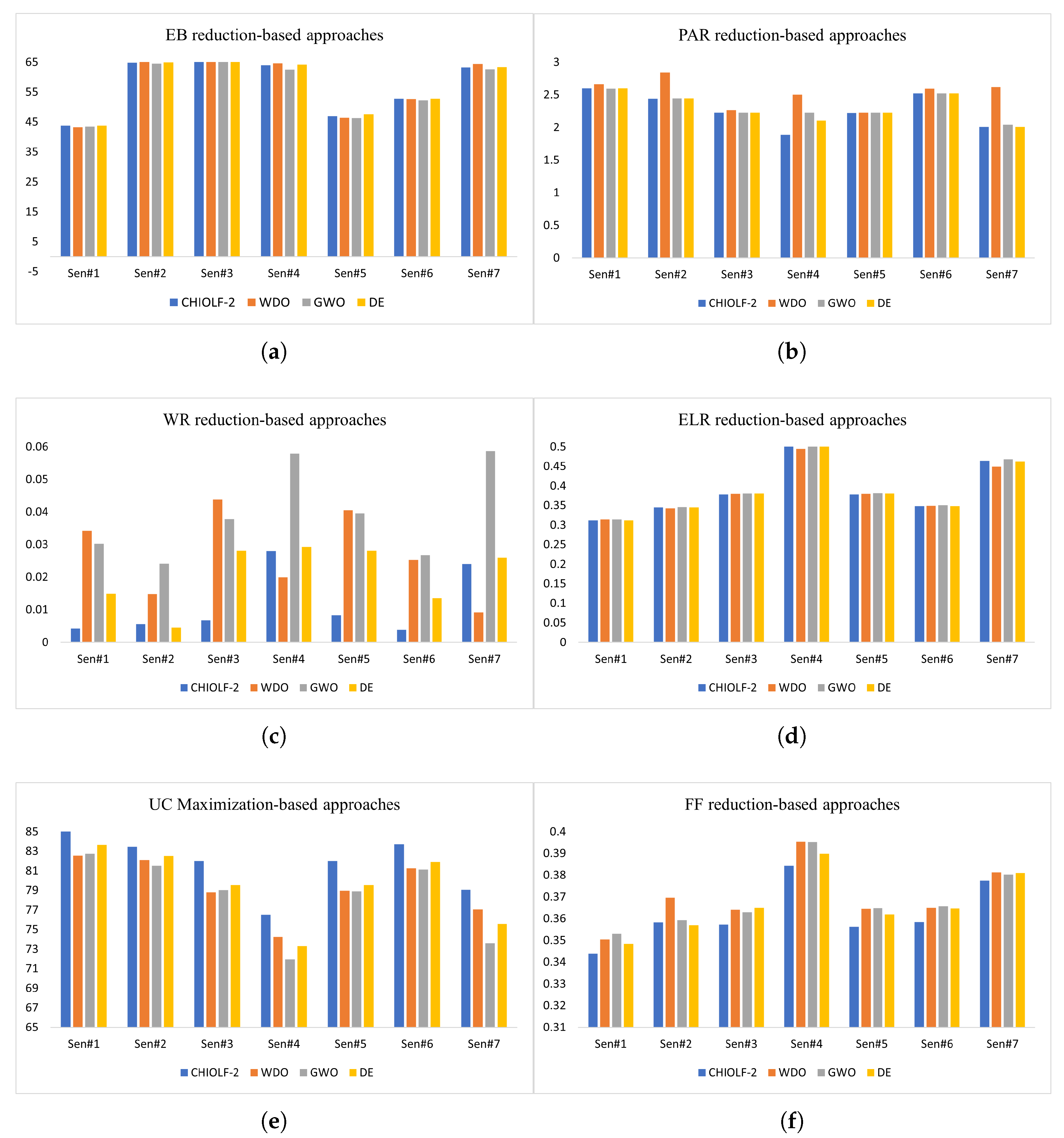Figure 4 presents the performance comparison of different multi-objective algorithms on different scenarios.

Therefore, CHIOLF-2 demonstrated its superiority in maximizing user comfort level and significant performance in attaining better FF reduction. Thus, CHIOLF-2 introduces adaptive randomization behavior that improves population diversity and reduces stagnation probability by integrating Lévy Flight. Moreover, the Lévy distribution operator robustifies the exploration capability of the CHIO algorithm by improving individuals’ susceptibility to finding promising solutions to wellness in the proposed CHIOLF-2 model. Hence, it provides an efficient scheduling approach that balances aggressive interaction goals like appliance automation, visual comfort, and smart-grid requirements while managing uncertainty and scheduling complexity.

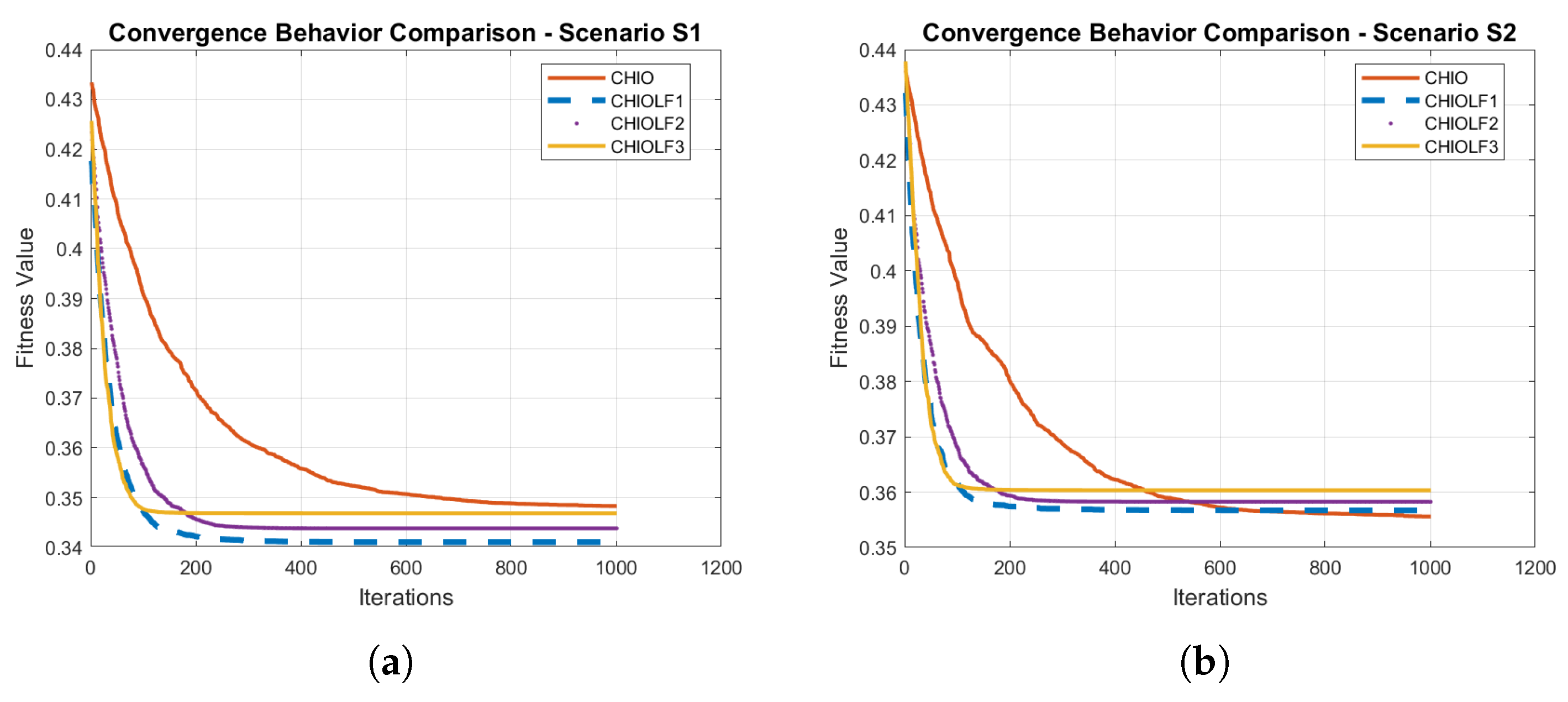
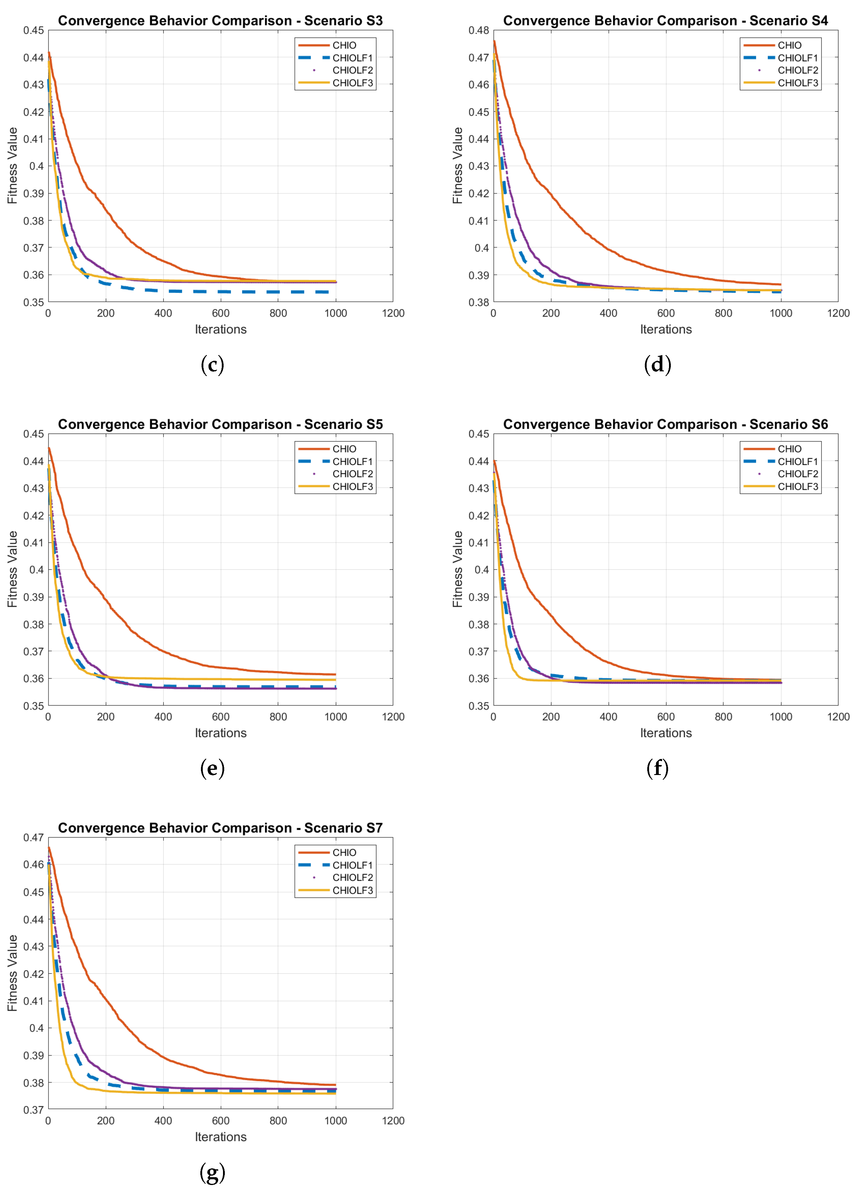
To show a performance comparison between the proposed CHIOLFs and the standard CHIO algorithm, Figure 5 presents a performance comparison of different multi-objective optimization methods, such as CHIOLF-1, CHIOLF-2, CHIOLF-3, and CHIO, according to the convergence behavior of fitness values for seven scenarios. The comparison results demonstrate that the CHIO-LF models have outperformed significantly among the naive CHIO algorithm across all evaluated scenarios except scenario no. two. This is due to the CHIO-LF models’ efficient trade-off between global exploration and local exploitation in finding the optimal solution. Thus, they attained better objective function values and better AESPSH schedules upon multi-objective optimization goals. 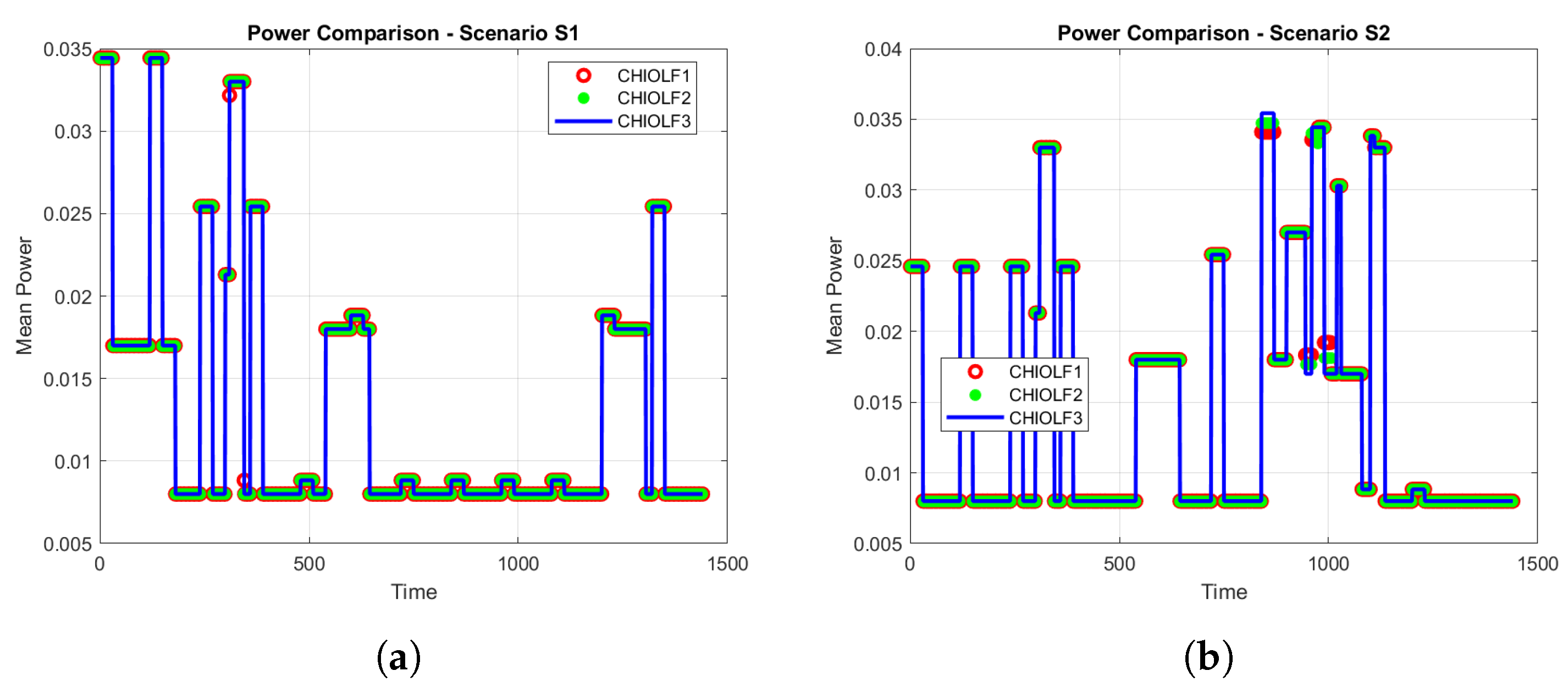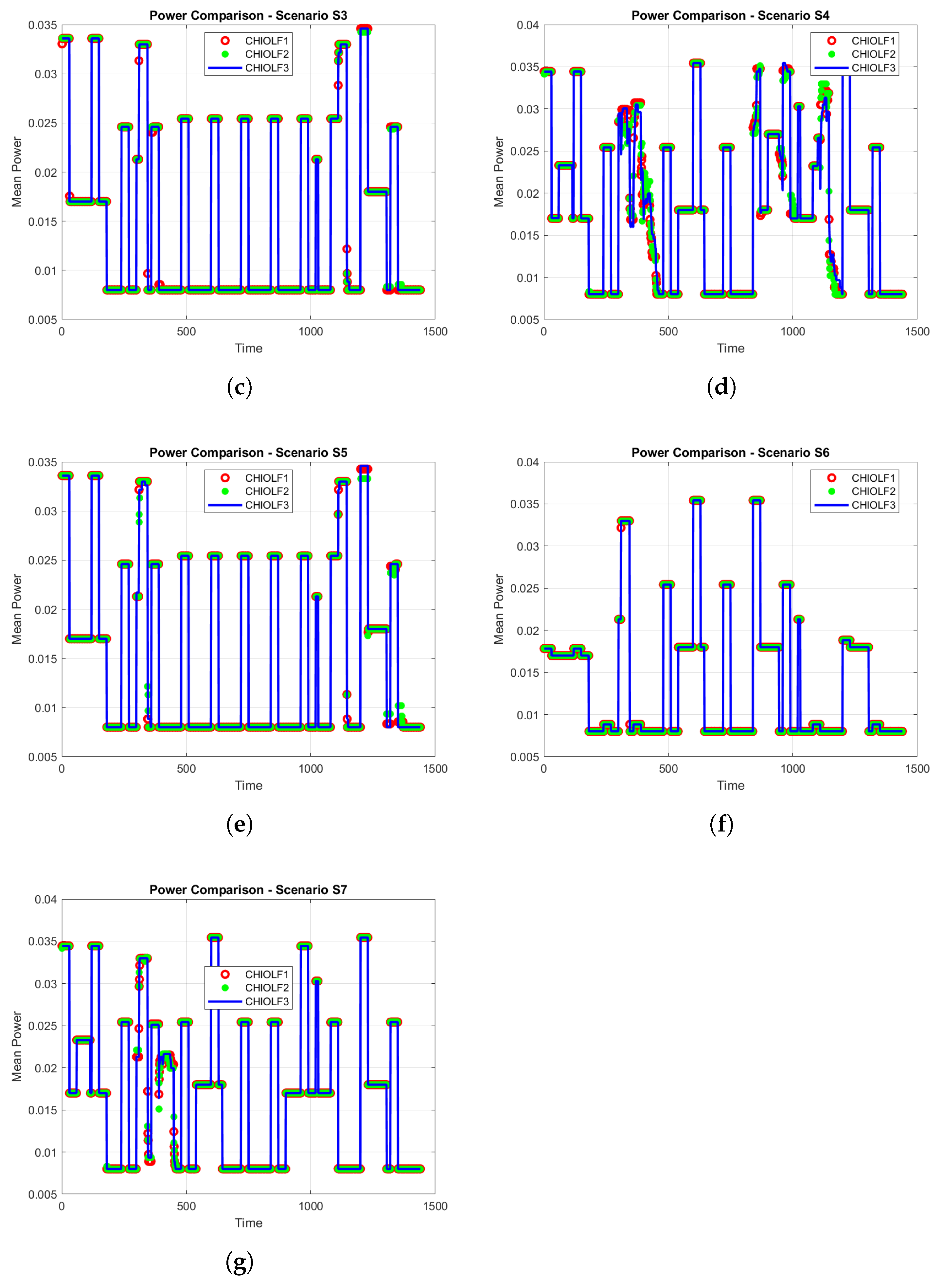Figure 6 shows a comparison of power optimization results between the hybrid CHIOLFs model and CHIO algorithms on different scenarios.

5. Conclusions and Future Works

In IoT appliances enabled modern smart homes for energy management, the escalating residential energy demand and grid instability remain a challenge. To overcome this, the current study tries to establish an optimal balance between state-space exploration and exploitation by introducing an integration of the CHIO algorithm with the LF optimizer. This study produced a structural integration of LF into targeted subpopulation phases of CHIO to avoid the algorithm’s tendency for premature convergence by establishing an optimal balance between state-space exploration and exploitation. Alongside, three structural hybridization models (independent variables) were evaluated against high-resolution economic and operational metrics: Electricity Bill (EB) cost, Peak-to-Average Ratio (PAR), Waiting Rate (WR), and Energy Limit Rate (ELR) (dependent variables). The mechanism used was that the heavy-tailed, adaptive randomization of LF would induce necessary population diversity, thereby allowing search agents to consistently escape local optima. Finally, this framework was tested by deploying the hybrid algorithms within a simulated Appliance Energy Scheduling Problem in Smart Home (AESPSH) environment, dynamically comparing their performance against the native CHIO algorithm and three state-of-the-art baselines (WDO, GWO, and DE).

This study answers the core scientific question posed in the introduction by evaluating the proposed CHIO-LFs comprehensive framework. The LF was integrated into three variant subpopulation phases, yielding three distinct models: the first CHIOLF-1 model, which was engineered to accelerate convergence and avoid CHIO stagnation; the second CHIOLF-2 model, designed to balance the exploration and exploitation of the evolutionary search space; and finally, the third hybridized CHIOLF-3 model, tailored to inject CHIO with the LF optimizer to increase the accuracy of finding promising solutions. The experimental findings demonstrate that the second hybridized CHIOLF-2 model attained an optimal architectural solution. By integrating LF to introduce adaptive randomization behavior, CHIOLF-2 effectively reduced the stagnation probability, achieving the highest performance in terms of User Comfort (UC) levels and Fitness Function (FF) values among all proposed models.

This research introduces an extended value significantly beyond a standard algorithmic comparison. The robustness and superiority of the CHIOLF-2 model demonstrate its capability to master the complex, nonlinear trade-offs inherent in modern smart grids. While state-of-the-art algorithms struggled with multidimensional conflicts, the CHIOLF-2 managed to strike the best possible balance between competing objectives, minimizing grid-level strain (EB cost and PAR) without compromising the end-user experience (maximizing comfort through optimized WR and ELR metrics). Thus, this study provides a highly efficient, grid-interactive scheduling method that successfully balances aggressive interaction goals, such as appliance automation and visual comfort, with stringent smart-grid requirements, all while effectively managing stochastic uncertainty and scheduling complexity.

For future work, the proposed CHIOLF-2 approach are highly recommended for solving NP-hard and real-world problems, such as feature and gene selection in medical applications. Furthermore, additional local search techniques are recommended to be hybridized with the CHIO algorithm for further investigation and to obtain improved results.

References

- Makhadmeh, S.N.; Khader, A.T.; Al-Betar, M.A.; Naim, S. An optimal power scheduling for smart home appliances with smart battery using grey wolf optimizer. In Proceedings of the 2018 8th IEEE International Conference on Control System, Computing and Engineering (ICCSCE), Penang, Malaysia, 23–25 November 2018; IEEE: New York, NY, USA, 2018; pp. 76–81. [Google Scholar]
- Khalid, A.; Javaid, N.; Guizani, M.; Alhussein, M.; Aurangzeb, K.; Ilahi, M. Towards dynamic coordination among home appliances using multi-objective energy optimization for demand side management in smart buildings. IEEE Access 2018, 6, 19509–19529. [Google Scholar] [CrossRef] [Scilit]
- Al-Odat, Z.A.; Srinivasan, S.K.; Al-qtiemat, E.; Dubasi, M.A.L.; Shuja, S. Iot-based secure embedded scheme for insulin pump data acquisition and monitoring. arXiv 2018, arXiv:1812.02357. [Google Scholar]
- Khan, M.A.; Salah, K. IoT security: Review, blockchain solutions, and open challenges. Future Gener. Comput. Syst. 2018, 82, 395–411. [Google Scholar] [CrossRef] [Scilit]
- Yan, Y.; Qian, Y.; Sharif, H.; Tipper, D. A survey on smart grid communication infrastructures: Motivations, requirements and challenges. IEEE Commun. Surv. Tutor. 2012, 15, 5–20. [Google Scholar]
- Sharda, S.; Singh, M.; Sharma, K. Demand side management through load shifting in IoT based HEMS: Overview, challenges and opportunities. Sustain. Cities Soc. 2021, 65, 102517. [Google Scholar] [CrossRef] [Scilit]
- Dehghani, M.; Bornapour, S.M. Smart homes energy management: Optimal multi-objective appliance scheduling model considering electrical energy storage and renewable energy resources. Heliyon 2025, 11, e42417. [Google Scholar] [CrossRef] [Scilit] [PubMed]
- Aslam, S.; Herodotou, H.; Mohsin, S.M.; Javaid, N.; Ashraf, N.; Aslam, S. A survey on deep learning methods for power load and renewable energy forecasting in smart microgrids. Renew. Sustain. Energy Rev. 2021, 144, 110992. [Google Scholar] [CrossRef] [Scilit]
- Taryudi; Adriano, D.B.; Ciptoning Budi, W.A. Iot-based integrated home security and monitoring system. J. Phys. Conf. Ser. 2018, 1140, 012006. [Google Scholar] [CrossRef] [Scilit]
- Feng, C.; Jumaah Al-Nussairi, A.K.; Chyad, M.H.; Sawaran Singh, N.S.; Yu, J.; Farhadi, A. AI powered blockchain framework for predictive temperature control in smart homes using wireless sensor networks and time shifted analysis. Sci. Rep. 2025, 15, 18168. [Google Scholar] [CrossRef] [Scilit] [PubMed]
- Lakhan, A.; Alyasseri, Z.A.A.; Mohammed, M.A.; Al-Attar, B.; Nedoma, J.; Alubady, R.; Memon, S.; Martinek, R. Sustainable secure blockchain assisted AIoT and green multi-constraints supply chain system. IEEE Internet Things J. 2025, 21, 39392–39406. [Google Scholar] [CrossRef] [Scilit]
- Wang, X.; Mao, X.; Khodaei, H. A multi-objective home energy management system based on internet of things and optimization algorithms. J. Build. Eng. 2021, 33, 101603. [Google Scholar] [CrossRef] [Scilit]
- AL-Shammri, F.K.; Noman Obeid, H.; Abbas, M.S.; Mohammed, A.S.; Alzamili, Z.; Aleigailly, M.A.; Ali Hasan, K.; Çelebi, F.V. Developing healthcare using Internet of Things (IoT): A survey of applications, challenges and future directions. Proc. BIO Web Conf. 2024, 97, 00004. [Google Scholar] [CrossRef] [Scilit]
- Teng, M.; Al-Hamdawee, Z.M.A.; Ali, A.B.; Jin, K.; Ahmadi, M. Integrating digital twins and neural networks for real-time temperature management in smart homes: An innovative approach using ZigBee networks. Energy Rep. 2025, 13, 6201–6218. [Google Scholar] [CrossRef] [Scilit]
- Arasteh, H.; Hosseinnezhad, V.; Loia, V.; Tommasetti, A.; Troisi, O.; Shafie-Khah, M.; Siano, P. Iot-based smart cities: A survey. In Proceedings of the 2016 IEEE 16th International Conference on Environment and Electrical Engineering (EEEIC), Florence, Italy, 7–10 June 2016; IEEE: New York, NY, USA, 2016; pp. 1–6. [Google Scholar]
- Hosseini, S.M.; Carli, R.; Dotoli, M. Robust optimal energy management of a residential microgrid under uncertainties on demand and renewable power generation. IEEE Trans. Autom. Sci. Eng. 2020, 18, 618–637. [Google Scholar]
- Duman, A.C.; Erden, H.S.; Gönül, Ö.; Güler, Ö. A home energy management system with an integrated smart thermostat for demand response in smart grids. Sustain. Cities Soc. 2021, 65, 102639. [Google Scholar] [CrossRef] [Scilit]
- Makhadmeh, S.N.; Khader, A.T.; Al-Betar, M.A.; Naim, S.; Abasi, A.K.; Alyasseri, Z.A.A. Optimization methods for power scheduling problems in smart home: Survey. Renew. Sustain. Energy Rev. 2019, 115, 109362. [Google Scholar] [CrossRef] [Scilit]
- Yang, Q.; Wang, H. Privacy-preserving transactive energy management for IoT-aided smart homes via blockchain. IEEE Internet Things J. 2021, 8, 11463–11475. [Google Scholar] [CrossRef] [Scilit]
- Rehman, A.U.; Wadud, Z.; Elavarasan, R.M.; Hafeez, G.; Khan, I.; Shafiq, Z.; Alhelou, H.H. An optimal power usage scheduling in smart grid integrated with renewable energy sources for energy management. IEEE Access 2021, 9, 84619–84638. [Google Scholar] [CrossRef] [Scilit]
- Bakare, M.S.; Abdulkarim, A.; Zeeshan, M.; Shuaibu, A.N. A comprehensive overview on demand side energy management towards smart grids: Challenges, solutions, and future direction. Energy Inform. 2023, 6, 4. [Google Scholar] [CrossRef] [Scilit]
- Usman, A.; Shami, S.H. Evolution of communication technologies for smart grid applications. Renew. Sustain. Energy Rev. 2013, 19, 191–199. [Google Scholar] [CrossRef] [Scilit]
- Elsayed, S.M.; Sarker, R.A.; Essam, D.L. A novel evolutionary algorithm for solving constrained optimization problems in engineering. Comput. Ind. Eng. 2011, 60, 74–85. [Google Scholar]
- Al-Betar, M.A.; Alyasseri, Z.A.A.; Awadallah, M.A.; Abu Doush, I. Coronavirus Herd Immunity Optimizer (CHIO). Neural Comput. Appl. 2021, 33, 5011–5042. [Google Scholar] [CrossRef] [Scilit] [PubMed]
- Makhadmeh, S.N.; Khader, A.T.; Al-Betar, M.A.; Naim, S.; Alyasseri, Z.A.A.; Abasi, A.K. Particle Swarm optimization Algorithm for Power Scheduling Problem Using Smart Battery. In Proceedings of the 2019 IEEE Jordan International Joint Conference on Electrical Engineering and Information Technology (JEEIT), Amman, Jordan, 9–11 April 2019; IEEE: New York, NY, USA, 2019; pp. 672–677. [Google Scholar]
- Makhadmeh, S.N.; Abasi, A.K.; Al-Betar, M.A.; Awadallah, M.A.; Doush, I.A.; Alyasseri, Z.A.A.; Alomari, O.A. A novel link-based multi-objective grey wolf optimizer for appliances energy scheduling problem. Clust. Comput. 2022, 25, 4355–4382. [Google Scholar] [CrossRef] [Scilit]
- Emary, E.; Zawbaa, H.M. Metaheuristic algorithms for optimization problems: A review. Appl. Soft Comput. 2020, 87, 105993. [Google Scholar]
- Fei, Z.; Li, B.; Yang, S.; Xing, C.; Chen, H.; Hanzo, L. A survey of multi-objective optimization in wireless sensor networks: Metrics, algorithms, and open problems. IEEE Commun. Surv. Tutor. 2017, 19, 550–586. [Google Scholar] [CrossRef] [Scilit]
- Cho, J.H.; Wang, Y.; Chen, R.; Chan, K.S.; Swami, A. A Survey on Modeling and Optimizing Multi-Objective Systems. IEEE Commun. Surv. Tutor. 2017, 19, 1867–1901. [Google Scholar] [CrossRef] [Scilit]
- Marler, R.T.; Arora, J.S. Survey of multi-objective optimization methods for engineering. Struct. Multidiscip. Optim. 2004, 26, 369–395. [Google Scholar] [CrossRef] [Scilit]
- Roy, S.; Chaudhuri, S.S. Cuckoo search algorithm using Lévy flight: A review. Int. J. Mod. Educ. Comput. Sci. 2013, 5, 10. [Google Scholar] [CrossRef] [Scilit]
- Simon, D. Evolutionary Optimization Algorithms: Biologically-Inspired and Population-Based Approaches to Computer Intelligence; Wiley: Hoboken, NJ, USA, 2013. [Google Scholar]
- Gunantara, N. A review of multi-objective optimization: Methods and its applications. Cogent Eng. 2018, 5, 1502242. [Google Scholar] [CrossRef] [Scilit]
- Farina, M.; Amato, P. Fuzzy optimality and evolutionary multiobjective optimization. In Proceedings of the International Conference on Evolutionary Multi-Criterion Optimization, Faro, Portugal, 8–11 April 2003; pp. 58–72. [Google Scholar]
- Makhadmeh, S.N.; Khader, A.T.; Al-Betar, M.A.; Naim, S. Multi-objective power scheduling problem in smart homes using grey wolf optimiser. J. Ambient Intell. Humaniz. Comput. 2019, 3643–3667. [Google Scholar] [CrossRef] [Scilit]
- López Jaimes, A.; Coello Coello, C.A. Some techniques to deal with many-objective problems. In Proceedings of the 11th Annual Conference Companion on Genetic and Evolutionary Computation Conference: Late Breaking Papers, Montréal, QC, Canada, 8–12 July2009; Association for Computing Machinery: New York, NY, USA, 2009; pp. 2693–2696. [Google Scholar]
- Rasheed, M.; Javaid, N.; Ahmad, A.; Khan, Z.; Qasim, U.; Alrajeh, N. An efficient power scheduling scheme for residential load management in smart homes. Appl. Sci. 2015, 5, 1134–1163. [Google Scholar] [CrossRef] [Scilit]
- Ullah, I.; Hussain, I.; Singh, M. Exploiting Grasshopper and Cuckoo Search Bio-Inspired Optimization Algorithms for Industrial Energy Management System: Smart Industries. Electronics 2020, 9, 105. [Google Scholar] [CrossRef] [Scilit]
- Manoharan, P.; Sinha, G.; Ravichandran, S.; Sin, T.C.; Hourani, A.O.; Hashim, T.J.T. Optimal appliance scheduling in a residential building using an improved binary algorithm with an inverse hyperbolic tangent function. Int. J. Electr. Power Energy Syst. 2026, 174, 111489. [Google Scholar] [CrossRef] [Scilit]
- Hafeez, G.; Javaid, N.; Iqbal, S.; Khan, F.A. Optimal residential load scheduling under utility and rooftop photovoltaic units. Energies 2018, 11, 611. [Google Scholar] [CrossRef] [Scilit]
- Javaid, N.; Javaid, S.; Abdul, W.; Ahmed, I.; Almogren, A.; Alamri, A.; Niaz, I. A hybrid genetic wind driven heuristic optimization algorithm for demand side management in smart grid. Energies 2017, 10, 319. [Google Scholar] [CrossRef] [Scilit]
- Ahmad, A.; Khan, A.; Javaid, N.; Hussain, H.M.; Abdul, W.; Almogren, A.; Alamri, A.; Azim Niaz, I. An optimized home energy management system with integrated renewable energy and storage resources. Energies 2017, 10, 549. [Google Scholar] [CrossRef] [Scilit]
- Qureshi, T.N.; Javaid, N.; Naz, A.; Ahmad, W.; Imran, M.; Khan, Z.A. A novel meta-heuristic hybrid enhanced differential harmony wind driven (EDHWDO) optimization technique for demand side management in smart grid. In Proceedings of the 2018 32nd International Conference on Advanced Information Networking and Applications Workshops (WAINA), Kraków, Poland, 16–18 May 2018; IEEE: New York, NY, USA, 2018; pp. 454–461. [Google Scholar]
- Ren, Z.; Chen, X.; Dong, Y. Two-stage optimization of appliance scheduling and BESS capacity with comfort level. Electr. Power Syst. Res. 2026, 255, 112771. [Google Scholar] [CrossRef] [Scilit]
- Sasanmoghadam, S.; Sabri-Laghaie, K. Adaptive scheduling and storage system preservation in smart home energy management systems: Considering cost efficiency, user satisfaction and storage systems durability. J. Energy Storage 2026, 142, 119521. [Google Scholar] [CrossRef] [Scilit]
- Zhao, Z.; Lee, W.C.; Shin, Y.; Song, K.B. An optimal power scheduling method for demand response in home energy management system. IEEE Trans. Smart Grid 2013, 4, 1391–1400. [Google Scholar] [CrossRef] [Scilit]
- Rahim, S.; Javaid, N.; Ahmad, A.; Khan, S.A.; Khan, Z.A.; Alrajeh, N.; Qasim, U. Exploiting heuristic algorithms to efficiently utilize energy management controllers with renewable energy sources. Energy Build. 2016, 129, 452–470. [Google Scholar] [CrossRef] [Scilit]
- Kumar, V.S.; Chatterjee, S. Optimized energy scheduling and trading in residential smart grids via renewable integration and Marine Predators Algorithm. Util. Policy 2026, 102, 102255. [Google Scholar] [CrossRef] [Scilit]
- Firouzabad, M.R.; Jahangir, M.H. Multi-objective optimization of residential energy scheduling using NSGA-II: A scenario-based weighted evaluation of thermal comfort, cost and environmental performance. Energy Rep. 2026, 16, 109528. [Google Scholar] [CrossRef] [Scilit]
- Yang, X.S.; Deb, S. Cuckoo search via Lévy flights. In Proceedings of the 2009 World Congress on Nature & Biologically Inspired Computing (NaBIC), Coimbatore, India, 9–11 December 2009; IEEE: New York, NY, USA, 2009; pp. 210–214. [Google Scholar]
- Farina, M.; Amato, P. A fuzzy definition of “optimality” for many-criteria optimization problems. IEEE Trans. Syst. Man. Cybern.—Part A Syst. Hum. 2004, 34, 315–326. [Google Scholar] [CrossRef] [Scilit]
- Makhadmeh, S.N.; Al-Betar, M.A.; Abasi, A.K.; Al-Redhaei, A.; Alomari, O.A.; Kouka, S. A hybrid marine predators algorithm with particle swarm optimization using renewable energy sources for energy scheduling problem-based IoT. Arab. J. Sci. Eng. 2024, 49, 12655–12678. [Google Scholar] [CrossRef] [Scilit]
- Central Maine Diesel, Wattage Calculator, 2017. Available online: http://www.centralmainediesel.com/wattage-calculator.asp (accessed on 28 July 2026).
- Ogwumike, C.; Short, M.; Abugchem, F. Heuristic optimization of consumer electricity costs using a generic cost model. Energies 2015, 9, 6. [Google Scholar] [CrossRef] [Scilit]
- Forsati, R.; Mahdavi, M.; Shamsfard, M.; Meybodi, M.R. Efficient stochastic algorithms for document clustering. Inf. Sci. 2013, 220, 269–291. [Google Scholar] [CrossRef] [Scilit]
Figure 1.
Architecture of Smart Home Based on Internet of Things Appliances.
Figure 2.
Flowchart of proposed hybrid Coronavirus Herd Immunity Optimizer with Lévy Flight models.
Figure 3.
Solution representation of the proposed hybrid Coronavirus Herd Immunity Optimizer with Lévy Flight models.
Figure 4.
Performance comparison of different multi-objective algorithms on different scenarios.
Figure 5.
Performance comparison of different Coronavirus Herd Immunity Optimizer models based on multi-objective algorithms in different scenarios.
Figure 6.
Power optimization results comparison of different Coronavirus Herd Immunity Optimizer models on different scenarios.