Generalised Equations for Calculating Arsenic Removal Efficiency Using Synthetic Adsorbents

Abstract

This study develops generalised equations to predict arsenic removal efficiency during adsorption using synthetic sand, based on two key factors: adsorbent dose and temperature. Previous experimental investigations demonstrated that iron oxide coated sand (IOCS), aluminium oxide coated sand (AOCS), and their mixtures are highly effective for arsenic removal. Best-fit equations were first derived for IOCS and AOCS at discrete temperatures as functions of dose concentration, and these were subsequently unified into single predictive equations capable of estimating removal efficiency across a wide range of temperatures and doses. The resulting models closely replicate experimental results, with correlation coefficients exceeding 0.99 for both IOCS and AOCS. Using the same methodology, an additional equation was developed for a 50:50 mixture of IOCS and AOCS, yielding a slightly lower but still strong correlation coefficient of 0.97. In contrast, linear proportioning of the individual IOCS and AOCS equations failed to accurately predict the removal efficiency of the mixed adsorbent, indicating that simple linear scaling is inadequate for representing the combined adsorption behaviour.

1. Introduction

It is well-established that prolonged consumption of arsenic-contaminated water causes several health-related issues. Therefore, WHO recommended a maximum limit of arsenic concentration in drinking water of 10 ppb (i.e., 0.01 mg/L) to avoid any health hazard [1]. Unfortunately, in many regions of the world, arsenic concentration in the only available drinking water is higher than this recommended limit, and it is evident that it causes severe skin diseases as well as pigmentation, neurological disorders, and cancer [2]. Although arsenic in the water can be present as both organic and inorganic forms, the inorganic form of arsenic has greater toxicity. As per chemical elements, arsenic can be present in four different forms; however, trivalent arsenite, As(III) and pentavalent arsenate, As(V) are the most common forms found in natural water [3,4]. In the presence of oxygen, organic arsenic converts to inorganic arsenic, i.e., As(V) and As(III) [5]. As its potential hazards have been exposed to the public for a few decades, there have been several studies on arsenic removal techniques, and their techniques widely varied regarding their underlying concepts. Among the various physicochemical techniques employed for the removal of arsenic from water the most common ones are adsorption methods, coagulation methods, and oxidation methods. Recently, an emerging technique named ‘membrane technology’ has been also employed [6], not only for arsenic removal, but for the removal of many pollutants (i.e., uranium). However, practical implementation of such technology is not an inexpensive option.

Castañeda et al. [7] applied the electrocoagulation technique for the removal of hydrated silica, arsenic, and phosphates from real groundwater using a cascade-shaped up-flow reactor with aluminium plates as electrodes. They also presented the influence of current density and linear flow rates in an EC reactor on the removal efficiencies. They achieved the best removal of arsenic (to 1.5 µg/L) through EC with a current density of 10 mA/cm² and linear flow rate of 1.2 cm/s. Goren and Kobya [8] investigated removal of arsenic through electrocoagulation and explored individual and combine effects of five anions (phosphate, silica, bicarbonate, fluoride, and boron) and operating time on the removal efficiency of arsenic. As cost implications are a major factor for the implementation of such systems, they have developed mathematical models for the estimations of cost and removal efficiency depending on all the variables mentioned above. Some researchers used oxidation techniques for the removal of arsenic from water [9,10]. With the aim of cost minimisation, Mohan et al. [9] employed solar oxidation and removal of arsenic (SORAS) experiments using polyethylene terephthalate (PET) bottles and achieved very good arsenic removal efficiency, although with a lower concentration (100 μg/L) of arsenic.

Considering cost and efficiency, the adsorption techniques are found to be more suitable for the removal of arsenic. Adsorption techniques were also found to be effective for the removal of other pollutants [11]. Khan and Imteaz [12,13], through using natural Skye sand as an adsorbent, demonstrated that a 90% removal of arsenic is achievable through adsorption even with a very high initial concentration (500 μg/L) of arsenic. Xiong et al. [14] applied a biological method using an iron oxyhydroxysulfate mineral, schwertmannite, for the adsorption of arsenic and achieved very good (110~115 mg/per gram of adsorbent) removal of As(III) and As(V). Villela-Martínez et al. [15] conducted a thorough study on the simultaneous removal of fluoride and arsenate from drinking water by bone char prepared from animal bones. They have presented the effects of operating conditions, water matrix, and presence of fluoride onto the arsenate adsorption capacity of bone char. Shaikh et al. [16] investigated both the As(III) and As(V) removal efficiencies through adsorption using biochar-based iron nanocomposites. They have experimented with the effect of different operating conditions (adsorbent dose, contact time, initial As concentration, pH, stirring rate, and temperature) on As removal efficiency. Many studies proposed use of nanoparticles, biochar, and/or artificial substances for the augmentation of natural arsenic removal efficiency [17,18]. Through investigating inherent properties of a natural Skye sand, which rendered excellent arsenic removal efficiency, Khan and Imteaz [19] proposed synthetic adsorbents made from iron oxide coated sand (IOCS) and aluminium oxide coated sand (AOCS), and their mixes with different proportions. With this synthetic sand they have achieved 100% removal of arsenic from drinking water.

For a wider industrial scale implementation of generation of such adsorbents, a thorough investigation under different operating conditions is required, which was presented in Khan and Imteaz [19]. However, in real-life production, the manufacturer may need to alter some of the operating conditions to optimise manufacturing costs or to overcome any other practical constraints. In fact, it is not feasible to run experiments repeatedly to determine achievable removal efficiency for new sets of experimental conditions. Development and use of generalised equations ideally can overcome the need to conduct repeated experiments, as these equations are able to predict arsenic removal efficiency for any combination of operating conditions through simple numerical calculations. This paper presents the development of the generalised equations for the prediction of arsenic removal efficiency using different synthetic adsorbents (IOCS, AOCS, and their mixture) under different operating conditions based on the rigorous experimental results presented in Khan and Imteaz [19]. Although some researchers [18] employed machine learning techniques for the prediction of arsenic removal efficiency, this is a pioneering attempt at developing such a type of simple mathematical model on the mentioned topic that can be easily used by any ordinary stakeholder.

2. Materials and Methods

The methodology used is mainly the development of parametric equations based on earlier experimental results. It is basically the development of generalised equations for predicting arsenic removal efficiency based on independent relationships between the arsenic removal efficiency and dose concentration under different temperatures, which were established through rigorous experimental measurements presented earlier by Khan and Imteaz [19] using synthetic sand samples. The IOCS sand was prepared with the fine fraction of quartz sand (150–300 micron), which was mixed with FeCl₃·H₂O and NaOH to make a Fe(III) suspension. Similarly, AOCS was prepared with the aid of the fine fraction of quartz sand (150–300 micron) added with AlCl₃·6H₂O and NaOH to make an Al(III) suspension. Batch experiments were performed with the aid of a rotary shaker (Ratek) in vertical plane at a rotational speed of 20 rpm. Various amounts of adsorbent (0.5 g to 2.5 g) were added to 50 mL arsenic-contaminated water in a conical shaped falcon tube. The initial arsenic concentration of the samples was 500 μg/L. The experiments were conducted for 8 h. The pH of the samples was adjusted to 7.0 by using 1 M HCl and/or 1 M NaOH. The samples were prepared in triplicate for each amount of adsorbent. All the batch experiments were carried out at 22 °C. Arsenic removal efficiencies were assessed for five different adsorbent doses (0.5 g, 1.0 g, 1.5 g, 2.0 g, and 2.5 g) and four different adsorbent drying temperatures (80 °C, 100 °C, 150 °C, and 200 °C). More details on the experimental conditions are outlined in Khan and Imteaz [19].

Equations were developed with two independent variables: dose concentration and temperature. The following sections describe methodologies applied for different variables separately. From the visual inspection of the experimental measurements for the effect of dose concentration on arsenic removal efficiency for a particular temperature, the pattern can be represented with an inverse exponential function, which diminishes with the increase of dose concentration and reaches to a maximum constant value for high dose concentration. Through several trials it was found that the following equation can best represent the experimental measurements:

$$RE={\displaystyle \frac{a}{b+e^{-c \ast d}}}$$

(1)

where, ‘RE’ is the arsenic removal efficiency in “%”, ‘d’ is the dose amount in 50 mL arsenic-contaminated water, and ‘a’, ‘b’ and ‘c’ are the constants and coefficient required to be established from experimental measurements. From the experimental measurements of Khan and Imteaz [19], it was observed that for different temperatures, the values of ‘a’, ‘b’ and ‘c’ linearly vary with the temperature as per the following format:

$$a, b, c=-m \ast \left(T\right)+n$$

(2)

where, ‘T’ is the reaction temperature during IOCS/AOCS production in “°C”, ‘m’ and ‘n’ are the slope and intercept of the linear relationship, respectively.

Finally, a single equation for removal efficiency incorporating both the factors (temperature and dose concentration) can be derived as per the following format:

$$RE={\displaystyle \frac{-m_1 \ast T+n_1}{(-m_2 \ast T+n_2)+e^{-(-m_3 \ast T+n_3) \ast d}}}$$

(3)

where, the subscripts ‘1’, ‘2’ and ‘3’ represents the values corresponding to the constant/coefficient ‘a’, ‘b’ and ‘c’, respectively. It is observed that the same equation format can be used for both the equations for IOCS and AOCS.

Removal efficiencies were calculated using the developed equations for specific dose concentrations and temperatures used in the original experiments. Altogether, for each adsorbent there were total twenty combinations of measurements comprising five different dose concentrations and four different temperatures. The values estimated through the developed equations were compared with the original experimental values.

Further to investigating individual IOCS and AOCS samples, the mix of IOCS and AOCS (50:50 ration) was also investigated. Following the same procedure as discussed above, a separate combined equation was also developed for the calculation of arsenic removal efficiency using mix of IOCS and AOCS samples. Eventually, an attempt was made to calculate the removal efficiency of the mentioned mix using just simple proportionate values from both the individual equations using the linear proportioning.

Accuracy of the developed model was assessed with the basic statistical error measures of root mean squared error (RMSE) and mean absolute error (MAE). The RMSE of any predicted values compared to the observed values is defined as follows:

$$RMSE=\sqrt{{\displaystyle \frac{{\sum _{i=1}^n(X_{obs, i}- X_{model, i})}^2}{n}}}$$

(4)

where, X_obs are observed/measured values, X_model is modelled values at time i, and ‘n’ is the number data. The mean absolute error (MAE) is defined as the sum of the absolute value of the differences between all the measured values and modelled values, divided by the total number of predictions as outlined below:

$$MAE={\displaystyle \frac{\sum _{i=1}^n(X_{obs, i}- X_{model, i})}{n}}$$

(5)

Moreover, in addition to presenting comparison scatter plots, to better visualise the discrepancies of the proposed equations, residual plots are presented.

3. Results

3.1. Equation for IOCS

Table 1. Arsenic removal efficiencies using IOCS under different temperatures and adsorbent doses.

Temperature (°C)	Dose (g per 50 mL)
	0.5	1	1.5	2	2.5
80	71	85	95	99	100
100	65	82	93	97	98
150	61	77	88	93	96
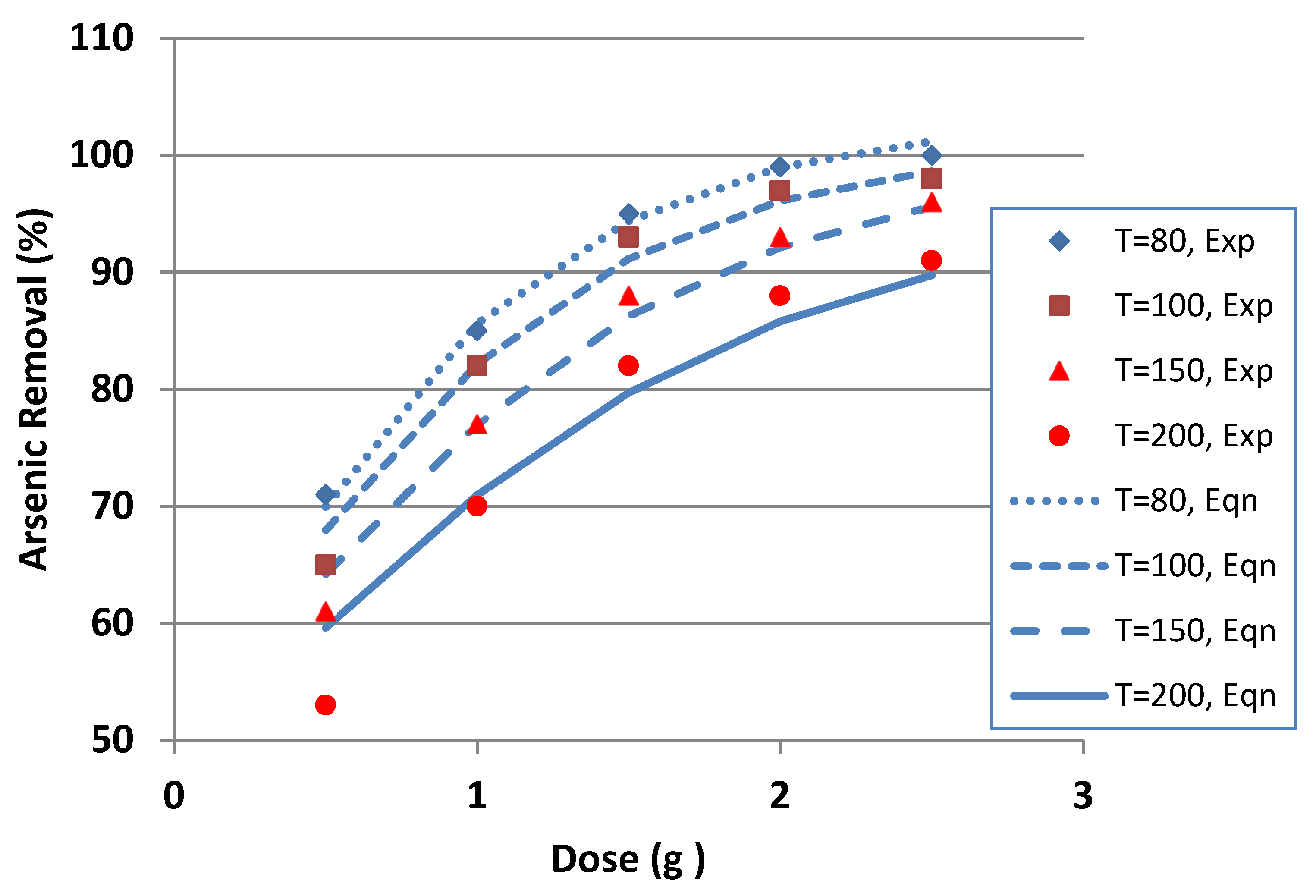
200	53	70	82	88	91

shows the experimental results on arsenic removal efficiencies obtained from different dose concentrations prepared under different temperatures. Data from each row of Table 1 can be represented by Equation (1), and there are four equations, one representing each temperature. Corresponding ‘a’, ‘b’ and ‘c’ values of Equation (1) for each temperature are tabulated in

Table 2. Coefficients of the best-fit equations for IOCS under different temperatures.

Temperature (°C)	Coefficient/Constant
	a	b	c
80	100	0.98	1.6
100	98	0.97	1.5
150	96	0.96	1.25
200	91	0.95	1.1

.

It was found that all the ‘a’, ‘b’ and ‘c’ values can be correlated with the temperature. Figure 1 shows the comparison between individual equation estimated results with the original experimental measurements. From the figure it is clear the individual equation can closely estimate the experimental results.

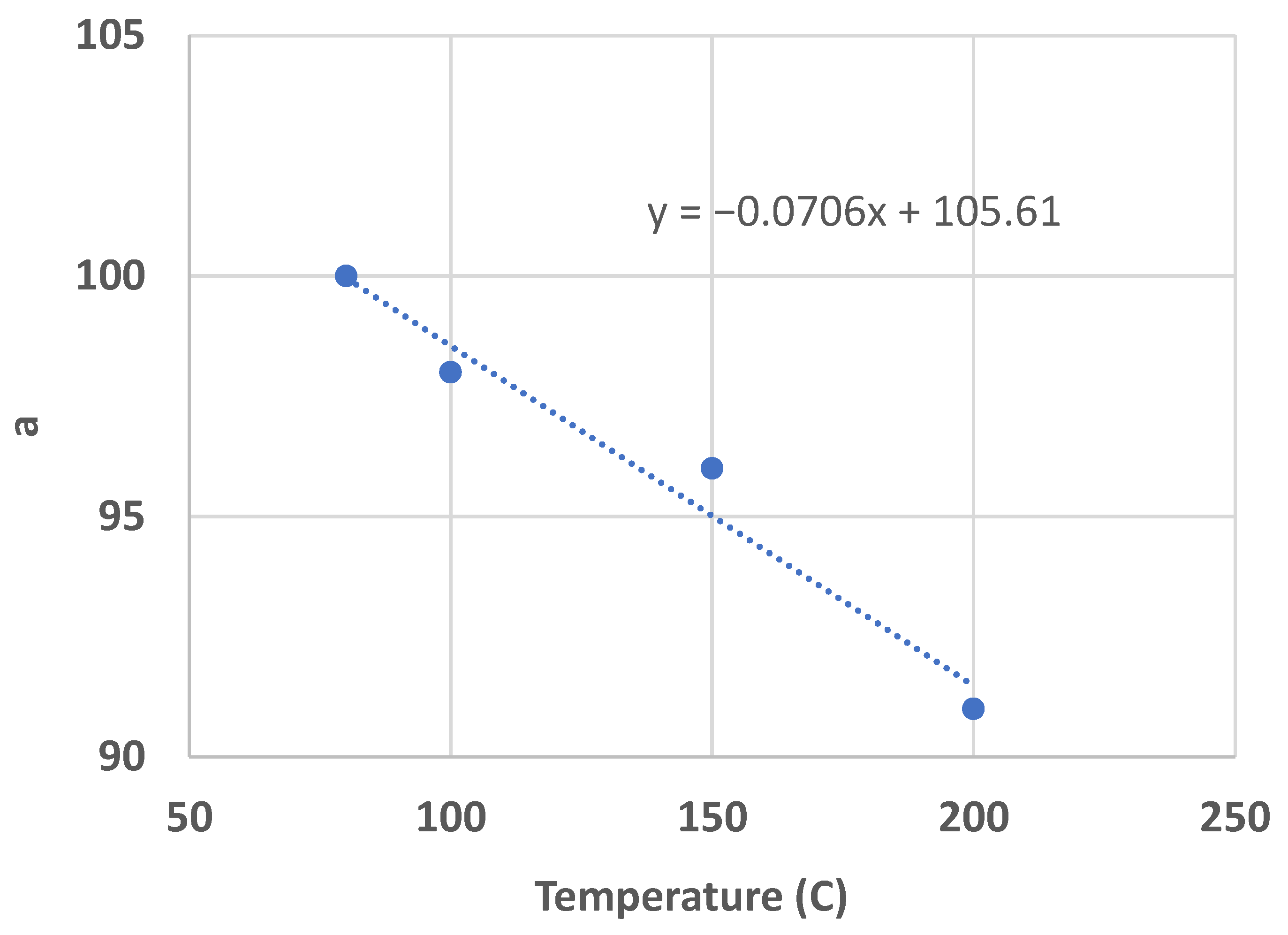
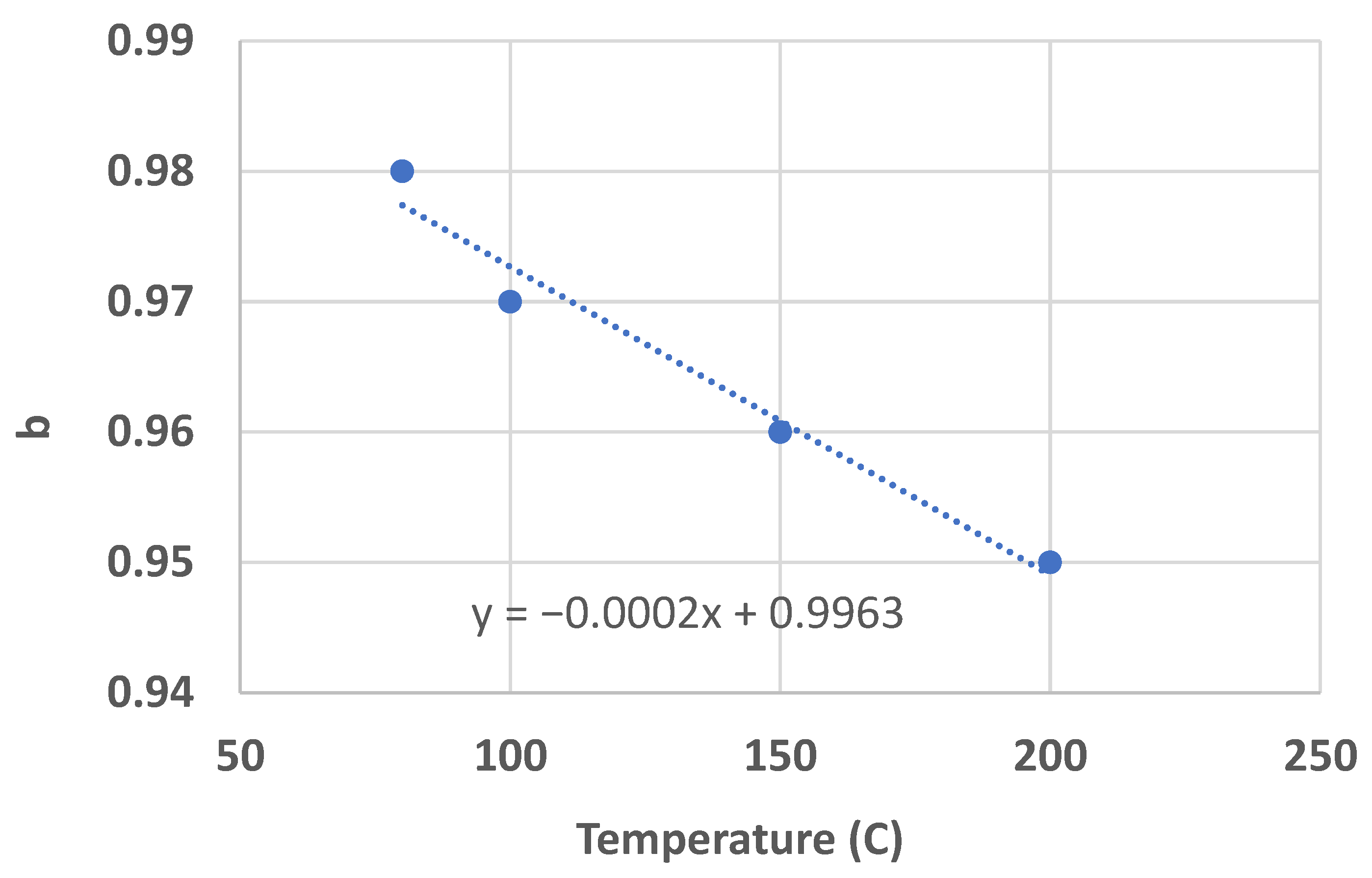
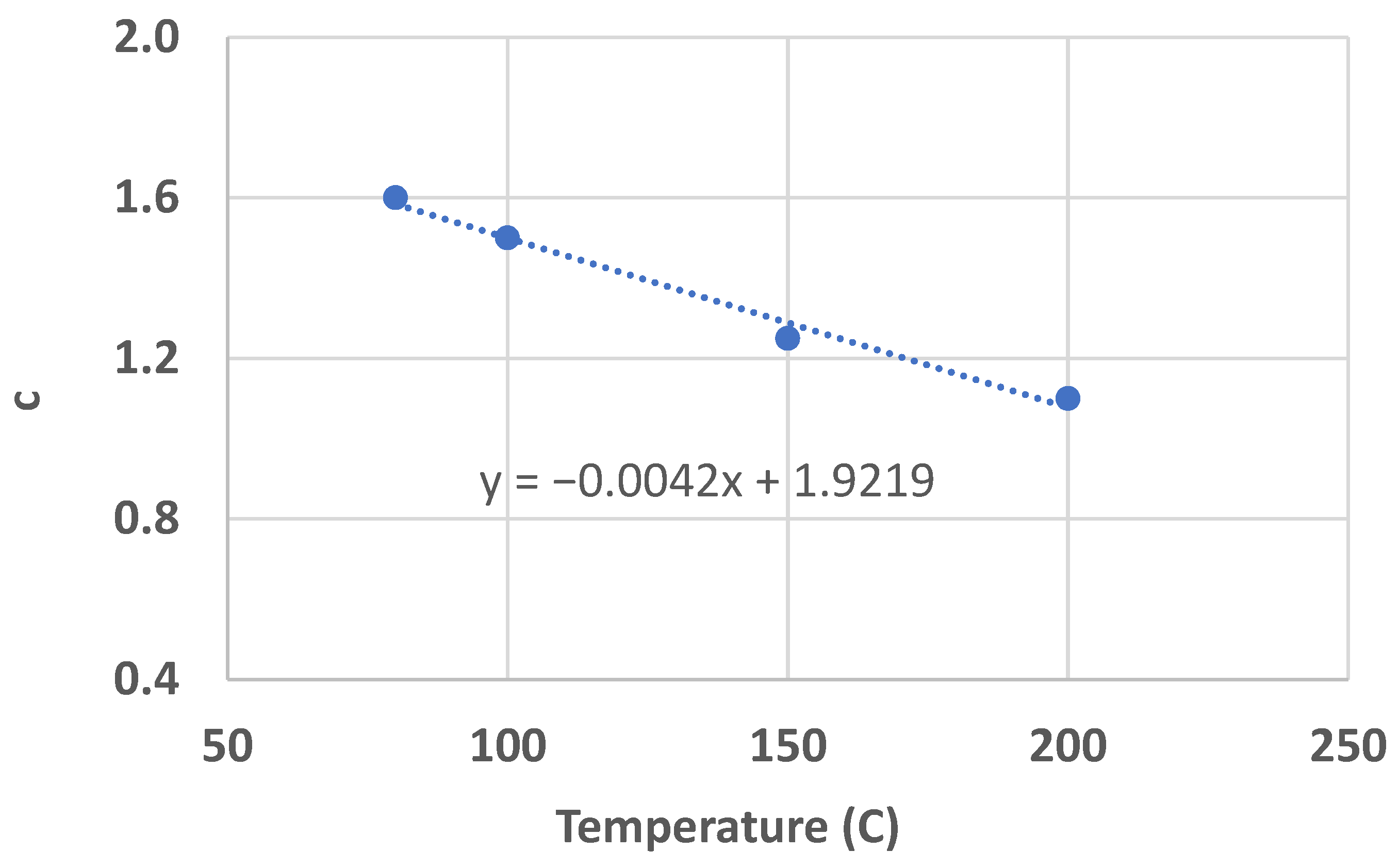
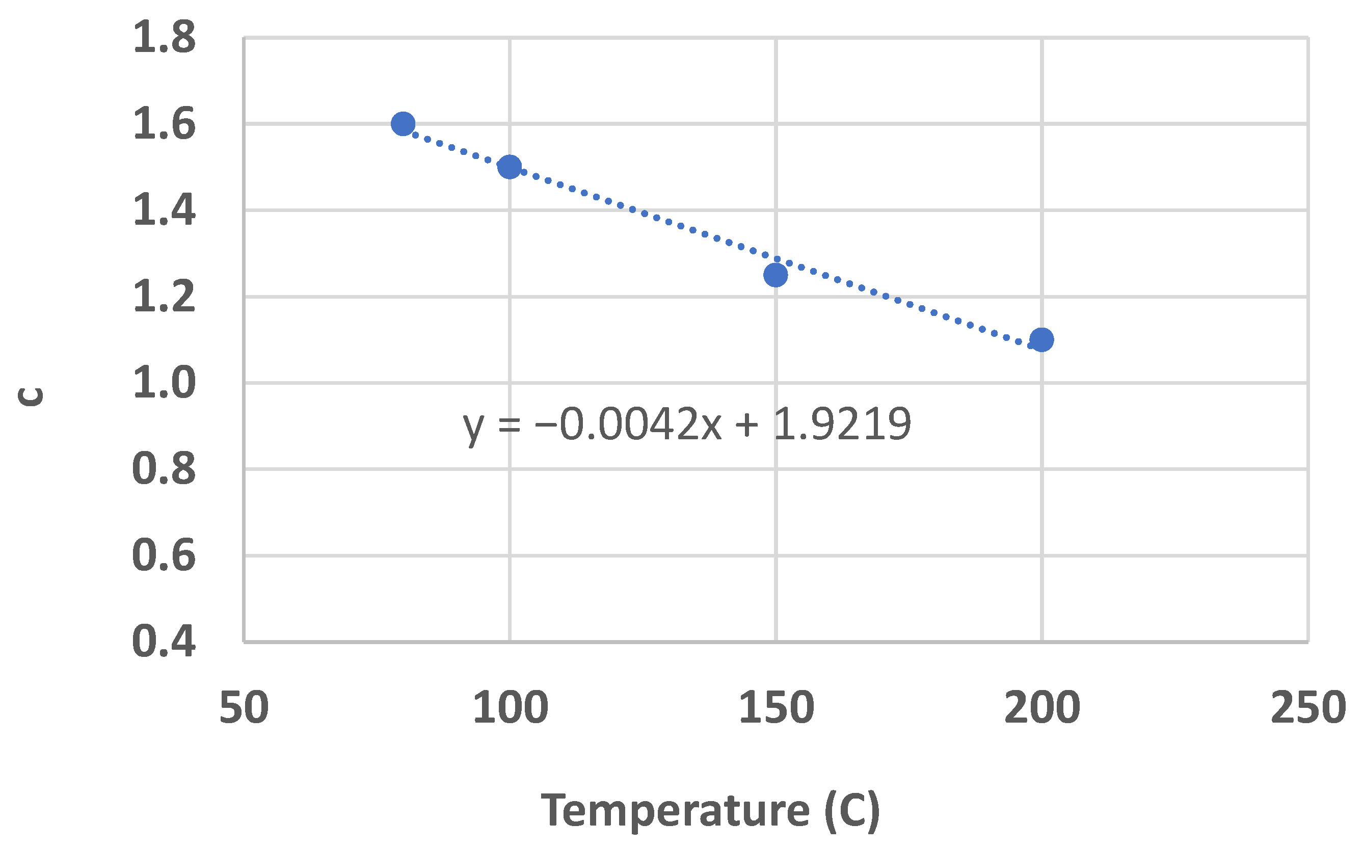
With the aim of developing a single generalised equation combining both the factors (dose concentration and temperature) Figure 2, Figure 3 and Figure 4 show the relationships between ‘a’, ‘b’ and ‘c’, respectively, with temperature. It is clear that all the figures can be represented with a linear line having a format shown in Equation (2). From the derived linear best-fit equations ‘a’, ‘b’ and ‘c’ can be expressed as follows:

$$a=-0.0706 \ast \left(T\right)+105.61$$

(6)

$$b=-0.0002 \ast \left(T\right)+0.9963$$

(7)

$$c=-0.0042 \ast \left(T\right)+1.9219$$

(8)

Replacing Equations (6)–(8) into Equation (3), the final single equation for the estimation of removal efficiency for IOCS would be:

$$RE={\displaystyle \frac{-0.0706 \ast \left(T\right)+105.61}{[-0.0002 \ast \left(T\right)+0.9963]+e^{-[-0.0042 \ast \left(T\right)+1.9219] \ast d}}}$$

(9)

Figure 5 shows the comparison of the single generalised equation (Equation (9)) estimated results with the original experimental measurements for different dose concentrations and temperatures. From the figure it is evident that the equation can closely estimate the experimental measurements. The correlation coefficient between the experimental measured and predicted values is 0.99, which is very high. Also, standard error estimates are low (RMSE = 2.22, MAE = 1.72).

To better visualise the discrepancies of the equation predicted values, Figure 6 shows the residual plot (i.e., deviations from the measured values) of the predicted plots. From the figure it can be seen all the predicted values lie within the deviations range of −3.0 to 2.70, except one value which was deviated by −6.5.

3.2. Equation for AOCS

Table 3. Arsenic removal efficiencies using AOCS under different temperatures and adsorbent doses.

Temperature (°C)	Dose (g per 50 mL)
	0.5	1	1.5	2	2.5
80	58	71	79	83	87
100	55	68	75	79	82
150	51	62	71	77	80
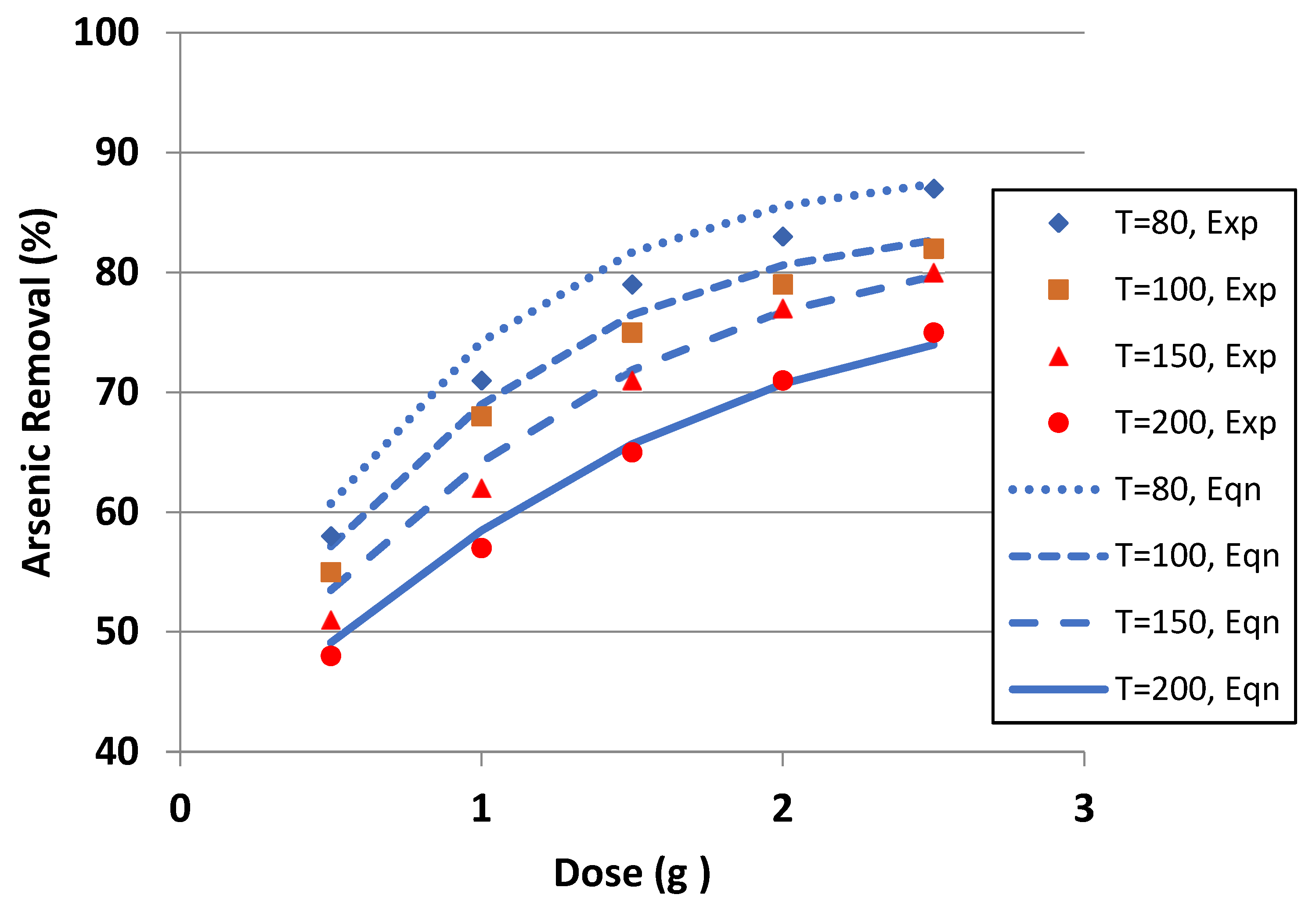
200	48	57	65	71	75

shows the experimental data on arsenic removal efficiencies obtained from different dose concentrations prepared under different temperatures. Data from each row of Table 3 can be represented by Equation (1) and there are four equations, one representing each temperature. Corresponding ‘a’, ‘b’ and ‘c’ values of Equation (1) for each temperature are tabulated in

Table 4. Coefficients of the best-fit equations for AOCS under different temperatures.

Temperature (°C)	Coefficient/Constant
	a	b	c
80	88	1.0	1.6
100	83	0.98	1.5
150	80	0.96	1.25
200	75	0.95	1.1

.

It is found that all the ‘a’, ‘b’ and ‘c’ values can be correlated with the temperature. Figure 7 shows the comparison between individual equation estimated results with the original experimental measurements. From the figure it is clear the individual equation can closely estimate the experimental results. With the aim of developing a single generalised equation combining both the factors (dose concentration and temperature), individual relationships between the temperature and the coefficients (a, b, c) were developed.

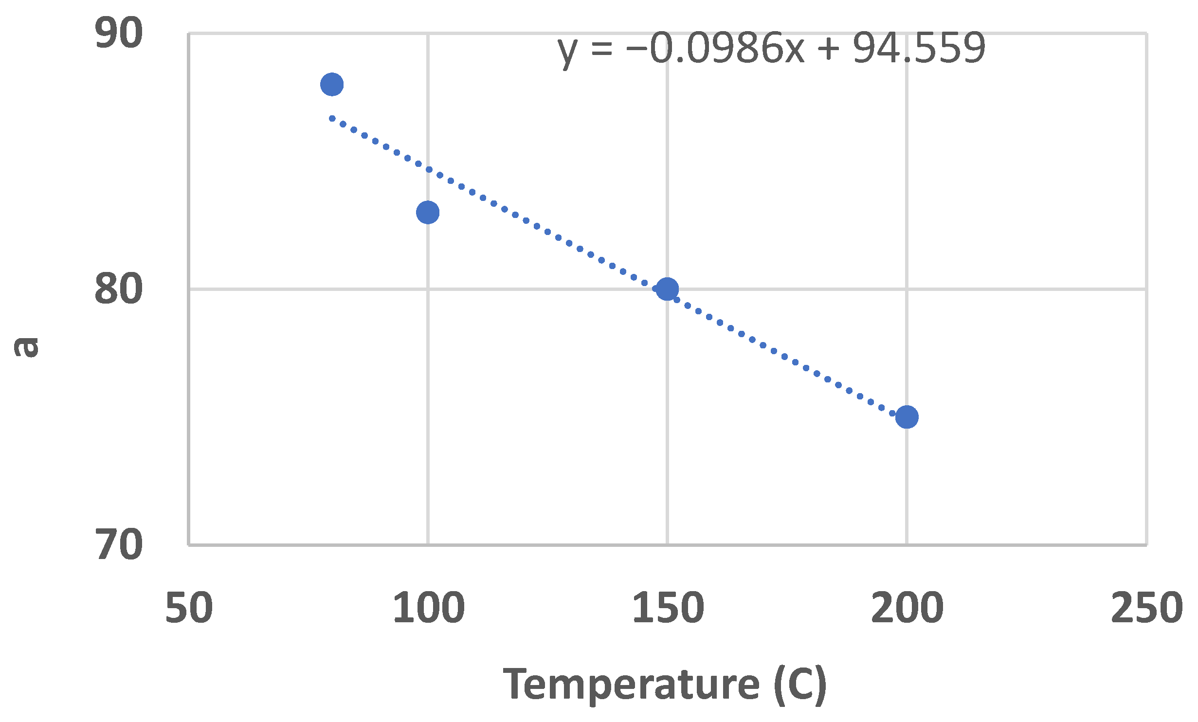
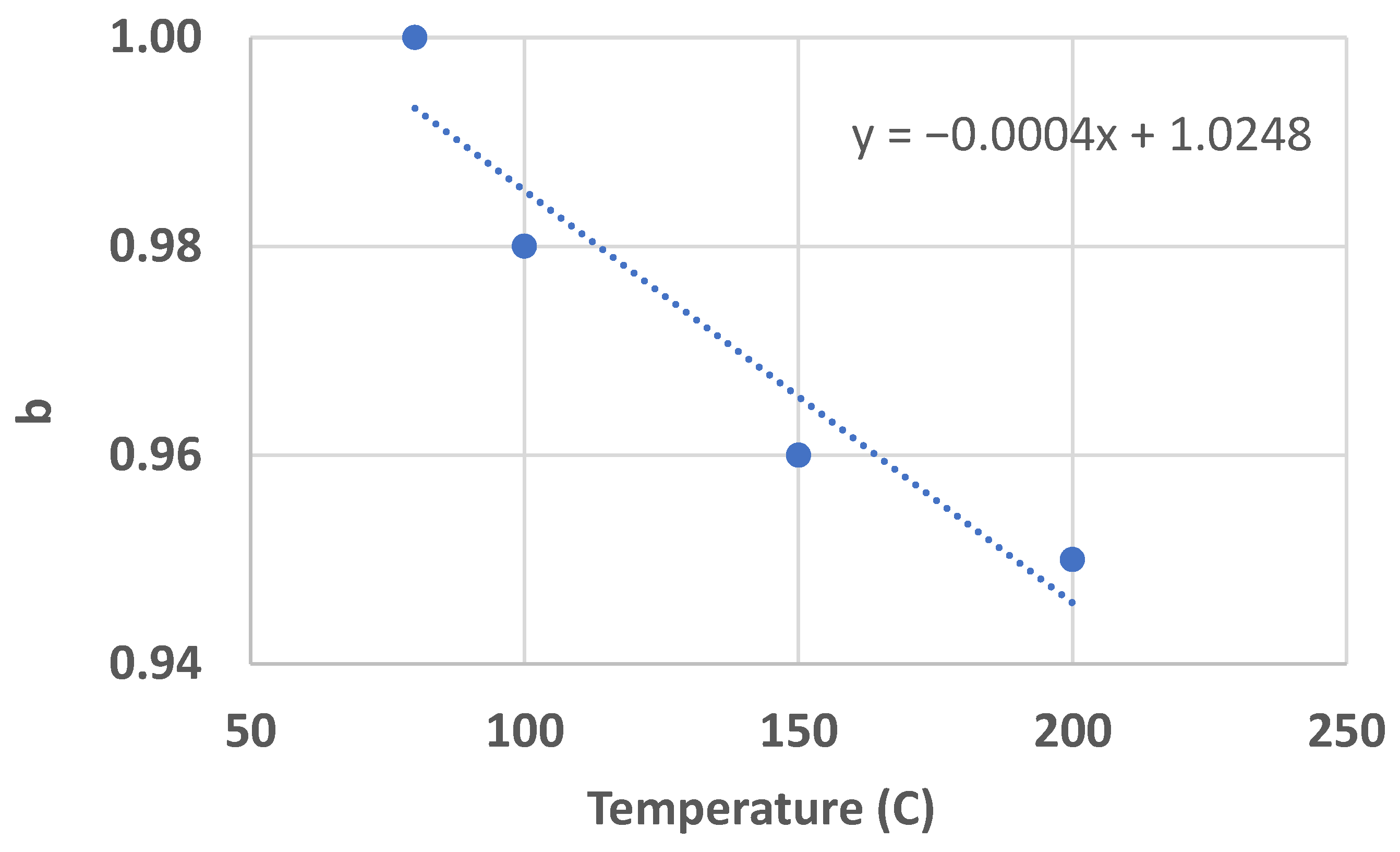
Figure 8, Figure 9 and Figure 10 show the relationships between ‘a’, ‘b’ and ‘c’, respectively, with temperature. It is clear that all the figures can be represented with a linear line having a format shown in Equation (2). From the derived linear best-fit equations ‘a’, ‘b’ and ‘c’ can be expressed as follows:

$$a=-0.0986 \ast \left(T\right)+94.55$$

(10)

$$b=-0.0004 \ast \left(T\right)+1.0248$$

(11)

$$c=-0.0042 \ast \left(T\right)+1.9219$$

(12)

Replacing Equations (10)–(12) into Equation (3), the final single equation for the estimation of removal efficiency for AOCS would be:

$$RE={\displaystyle \frac{-0.0986 \ast \left(T\right)+94.55}{[-0.0004 \ast \left(T\right)+1.0248]+e^{-[-0.0042 \ast \left(T\right)+1.9219] \ast d}}}$$

(13)

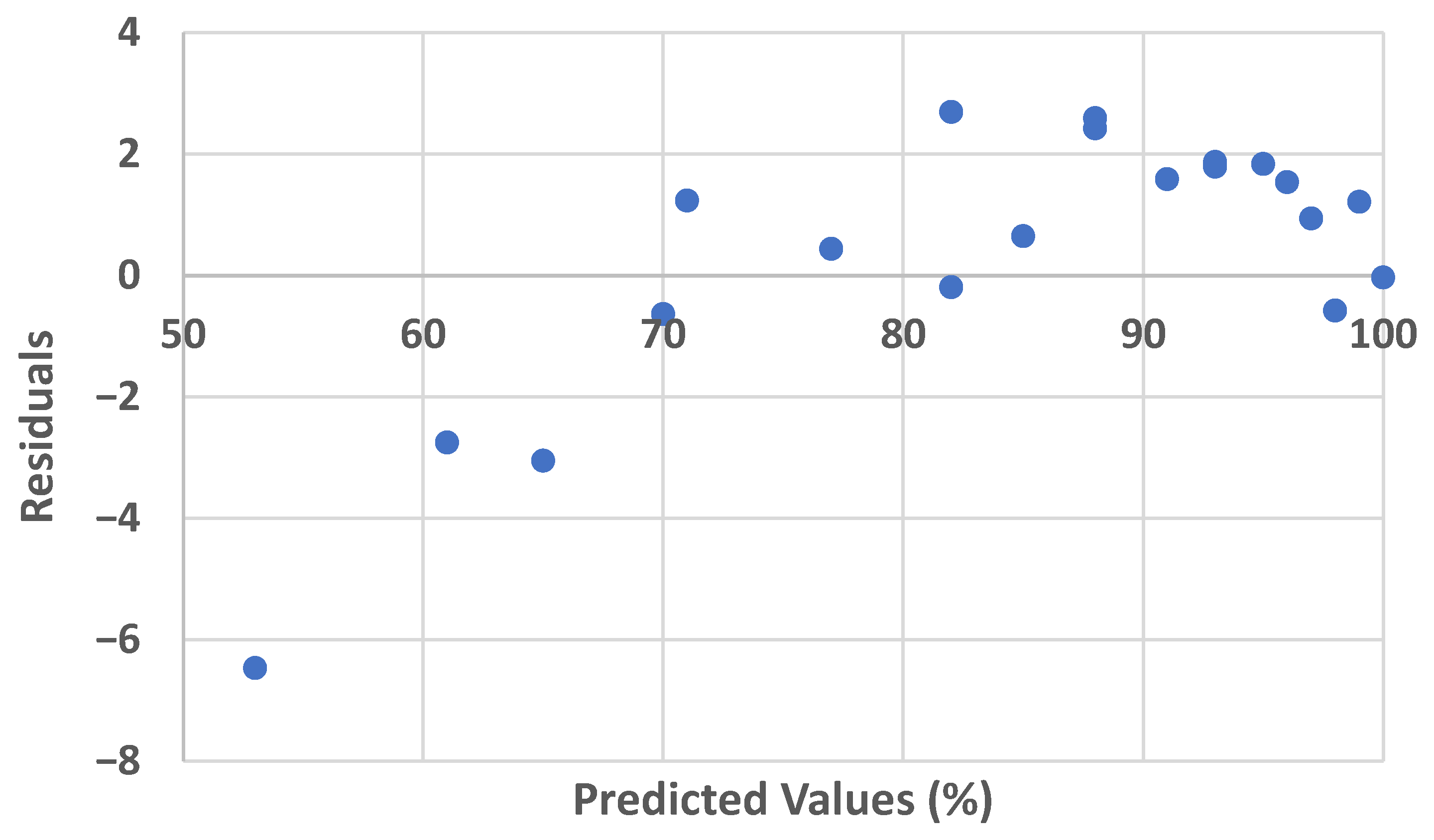
Figure 11 shows the comparison of the single generalised equation (Equation (13)) estimated results with the original experimental measurements for different dose concentrations and temperatures. From the figure it is evident that the equation can closely estimate the experimental measurements. The correlation coefficient between the experimental measured and predicted values is 0.99, which is very high. Also, standard error estimates are low (RMSE = 1.74, MAE = 1.51).

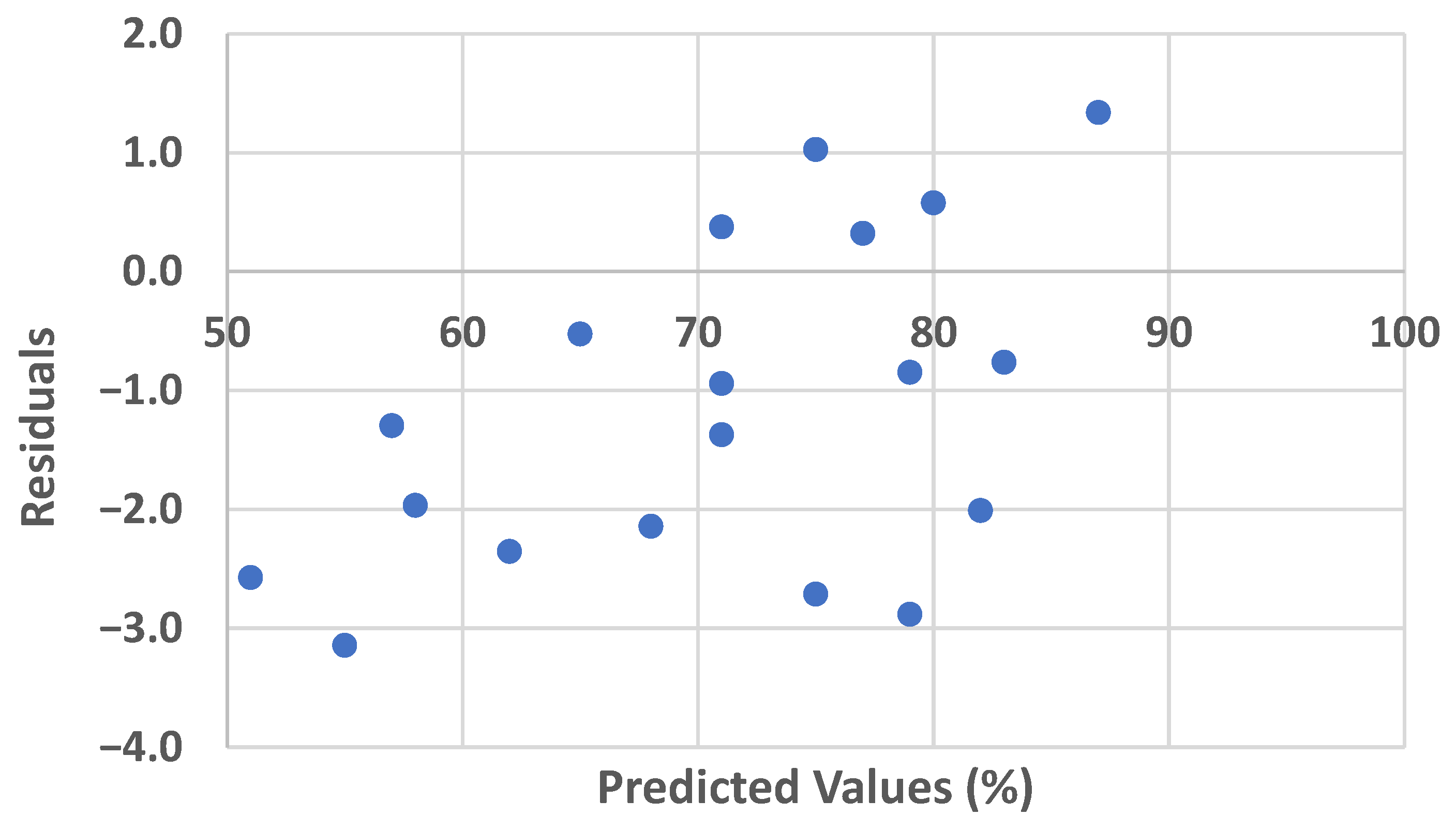
To better visualise the discrepancies of the equation predicted values, Figure 12 shows the residual plot (i.e., deviations from the measured values) of the predicted plots. From the figure it can be seen all the predicted values lie within the range of −3.1 to 1.30, which are very low compared to the predicted estimations of up to 90.

3.3. Equation for Mix of IOCS and AOCS

Following the same methodology described in the preceding sections for individual IOCS and AOCS samples, a separate combined equation was developed based on the experimental results using mixed IOCS and AOCS having a 50:50 ratio. From the derived best-fit equations, the following parameters can be found:

$$a=-0.1663 \ast \left(T\right)+104.28$$

(14)

$$b=-0.0005 \ast \left(T\right)+1.0426$$

(15)

$$c=-0.0042 \ast \left(T\right)+1.9219$$

(16)

Replacing Equations (14)–(16) into Equation (3), the final single equation for the estimation of removal efficiency for using mixed IOCS and AOCS would be:

$$RE={\displaystyle \frac{-0.1663 \ast \left(T\right)+104.28}{[-0.0005 \ast \left(T\right)+1.0426]+e^{-[-0.0042 \ast \left(T\right)+1.9219] \ast d}}}$$

(17)

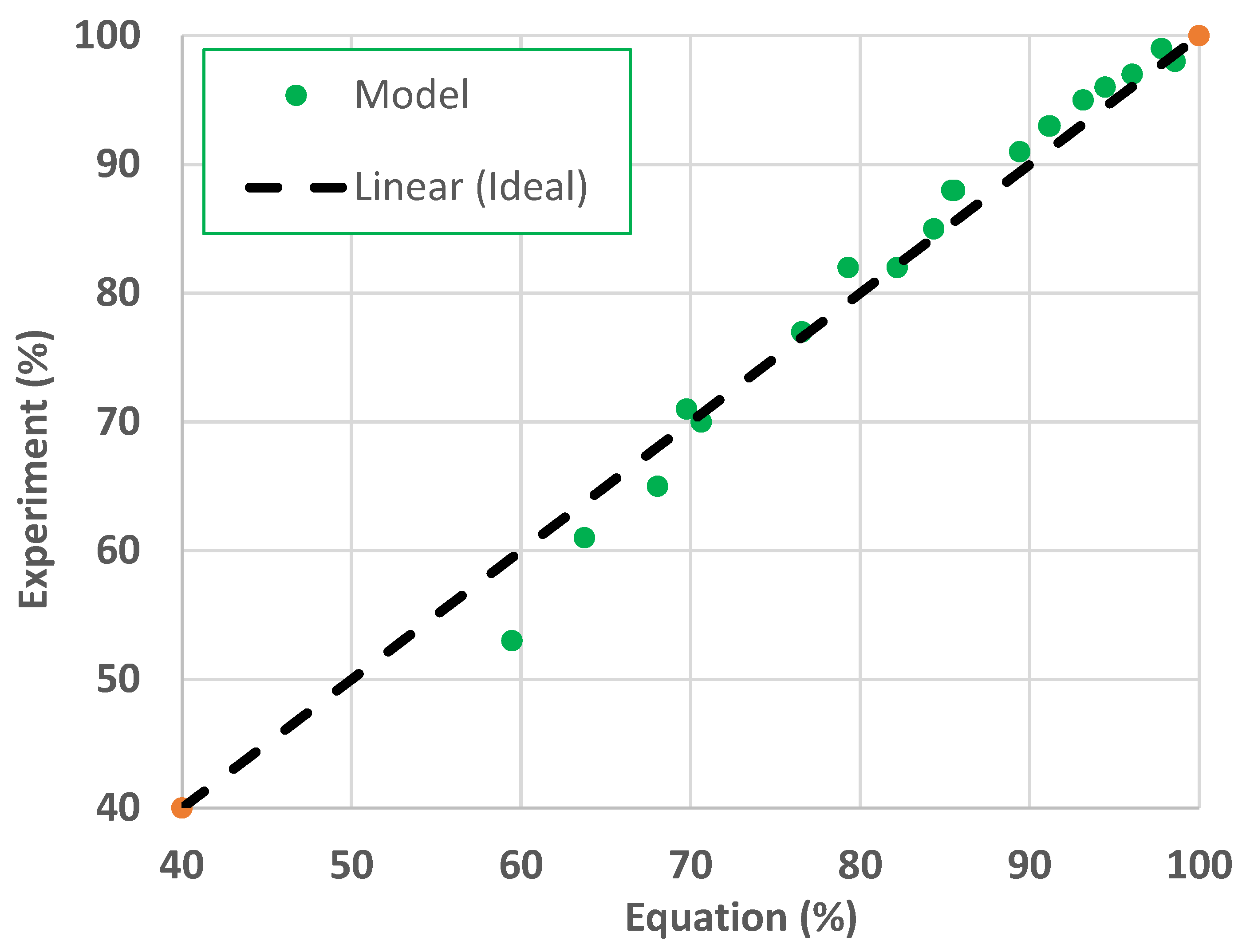
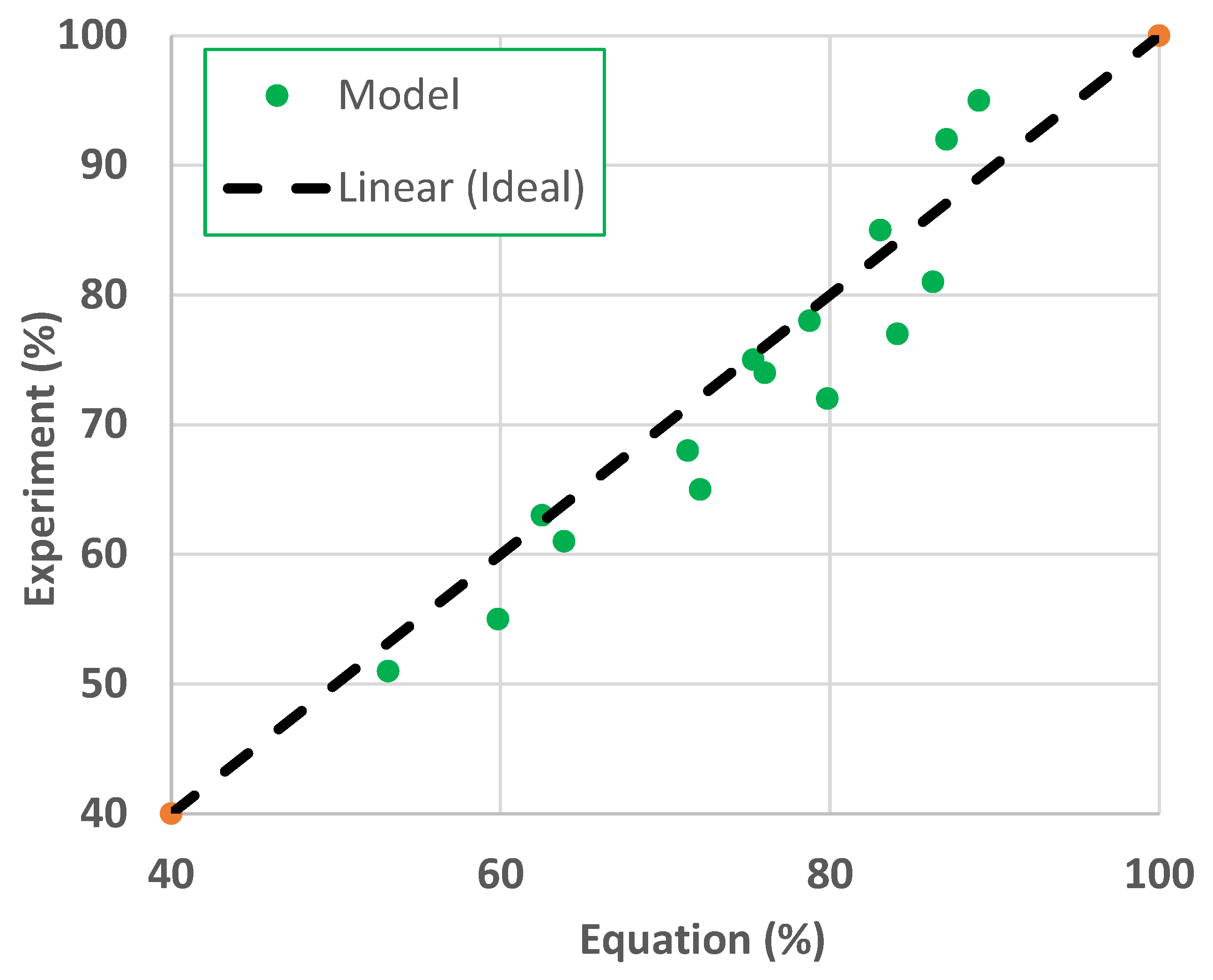
Figure 13 shows the comparison of the single generalised equation (Equation (15)) estimated results with the original experimental measurements for different dose concentrations and temperatures. From the figure it is evident that the equation can closely estimate the experimental measurements. The correlation coefficient of the estimations is 0.95. Standard error estimates of the predictions are higher compared to the estimations for individual samples (RMSE = 3.94, MAE = 3.06).

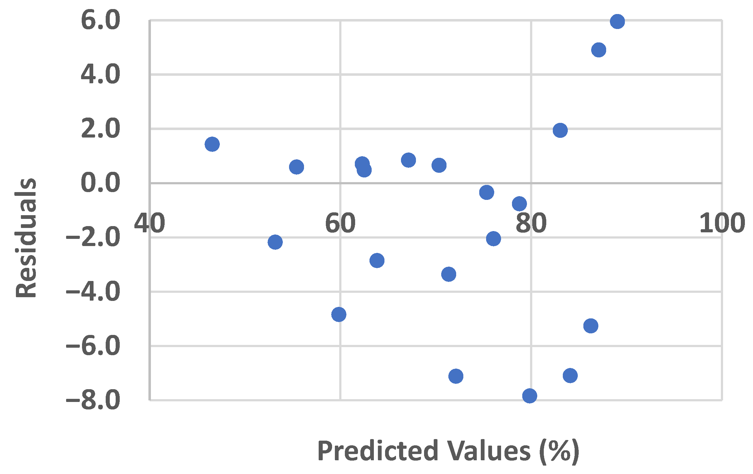
To better visualise the discrepancies of the equation predicted values, Figure 14 shows the residual plot (i.e., deviations from the measured values) of the predicted plot. From the figure it can be seen all the predicted values lie within the range of −7.8 to 5.90, which are higher compared to the residuals of the estimations using individual equations.

3.4. Calculation Using Linear Proportioning

The concept of such linear proportioning was just to convert estimations from IOCS and AOCS equations (explained in the earlier sections) using the used proportion. As per this linear proportioning the removal efficiency of the mixed sample is:

Removal Efficiency of IAOCS(I50A50) = 0.50 ∗ RE_IOCS + 0.50 ∗ RE_AOCS

(18)

where, RE_IOCS and RE_AOCS are the removal efficiencies of IOCS and AOCS, respectively, which are calculated through Equations (9) and (13), respectively.

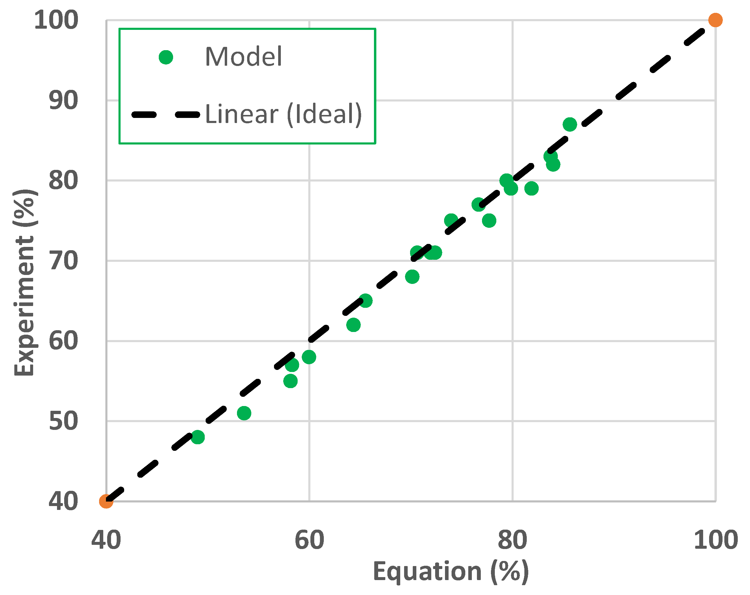
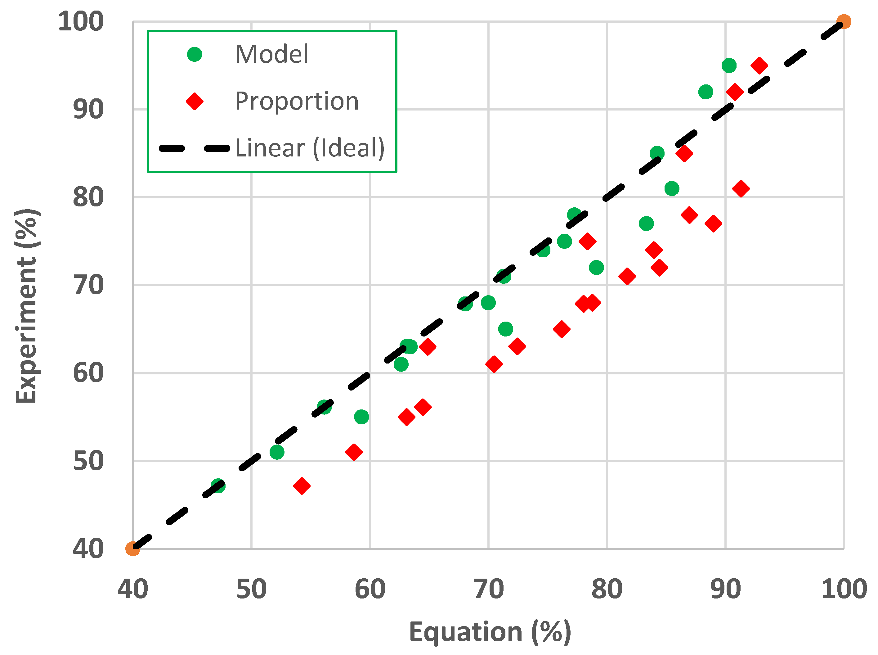
Figure 15 shows the comparison of Equation (18) estimated results with the original experimental measurements using IAOCS(I50A50) sample. From the figure it is clear that the proportioning calculation overestimates the removal efficiencies compared to the original experimental values. For the sake of comparison, Figure 15 also shows the values calculated through Equation (17). It can be seen from the figure that while Equation (17) estimated values closely match with the ideal line, Equation (18) calculated values are significantly below the ideal line. The RMSE value of the Equation (18) estimations is 8.6, whereas RMSE value of Equation (17) estimations is 3.94. This finding reveals that such proportioning calculation for complex chemical reactions is not likely to be accurate and effective.

4. Discussion

Experimental investigations into arsenic removal are extensive, with adsorption emerging as one of the most widely studied and effective methods. Numerous materials have been proposed as absorbents, with recent research increasingly emphasising sustainable options such as natural and recycled materials. Despite the breadth of experimental studies, large-scale and real-world applications remain limited. For stakeholders and manufacturers seeking wider implementation, it is essential to understand achievable arsenic removal efficiencies under varying operating conditions, particularly where practical constraints prevent operation at experimentally optimal settings. Consequently, the ability to reliably estimate removal efficiency across a range of conditions is critical. Generalised equations that incorporate key governing parameters provide a practical means to predict performance under different manufacturing and operational scenarios. As a pioneering effort in this area, the present study develops generalised equations based on temperature and adsorbent dose concentration.

It was found that developed equations including the equation for mixed sample are capable of accurately reproducing the experimental values. However, when a simple linear proportioning technique is used for the calculation of combined (IOCS + AOCS) sample from individual equations of each sample, the reproduced values were not matching with the measured values. Physio-chemical causes of this discrepancy are difficult to establish for a purely parametric model, which are solely based on change of pattern of individual variables and constants. For this case, the rate of change of efficiencies for IOCS sample was not same as the rate of change of efficiencies for the AOCS sample. As such, it is customary that such linear proportioning will not be accurate. Nonetheless, this was not the objective of this study; rather. the objectives were to develop parametric equations for the mentioned samples, which were successfully accomplished with very high accuracies.

It is to be noted that arsenic removal efficiency is also affected by some other factors such as pH, initial arsenic concentration, ionic strength etc. [20,21]. Consideration and inclusion of all those factors into one single equation would be a highly ambitious task. With additional experimental data generated using a similar framework considering more independent variables, further influencing factors can be integrated into the proposed modelling approach.

5. Conclusions

This study presented development of generalised equations for the estimation of arsenic removal efficiency from water through different synthetic sands (IOCS and AOCS), which were earlier established to be excellent adsorbents of arsenic from water. Based on earlier experimental results using those two synthetic sands, two generalised equations were derived that can estimate arsenic removal efficiency for any adsorbent dose at any temperature. Equations estimated results were compared with the original experimental results using IOCS and AOCS samples. It was found that both the equations for IOCS and AOCS can closely estimate the removal efficiency under any condition of dose concentration and temperature. Correlation coefficients of estimations for both the equations were more than 0.99. Moreover, regarding the standard error estimations, RMSE and MAE values of IOCS equation were 2.22 and 1.72, respectively, while RMSE and MAE values of AOCS equation were 1.74 and 1.51, respectively. Later, following the same procedure another equation was developed for the estimations of arsenic removal efficiency using a mix of IOCS and AOCS samples. The developed equation with the combined samples is also capable of closely estimating the experimental measurements with a correlation coefficient of 0.95. Among standard error values, RMSE and MAE values of the estimations using equation for combined samples were 3.94 and 3.06, respectively. Finally, to avoid the derivations of such complex parametric equations, it was attempted to estimate removal efficiency for the mixture of IOCS and AOCS samples using linear proportioning of materials used for the mixture. Individual removal efficiencies were calculated using separate IOCS and AOCS equations, and the final efficiency of the mix was calculated by summing the linear proportions of the individual equation produced results. It was found that such linear proportioning of the individually derived equations is unable to accurately estimate the removal efficiencies for the IOCS and AOCS mixture. RMSE value of the estimations using proportioning method was 8.6, whereas the RMSE value of the derived parametric equation was 3.94, revealing the fact that such linear proportioning is not likely to render accurate estimation for replication of complex chemical processes. Nonetheless, such generalised equations are very helpful for practical implementations of any such filter device, especially for manufacturers who would be able to optimise their input variables based on surrounding constraints. It is to be noted that developed equations are mainly valid for the range of temperatures 80~200 °C. It is recommended that future studies should endeavour to incorporate more independent variable(s) into such generalised equations. Also, as it is not wise to perform validation with the same set of experimental data, for the validation of the current proposed equation, future study should focus similar experimental study with the same adsorbents.

References

1. Ahmad, A.; van der Wens, P.; Baken, K.; de Waal, L.; Bhattacharya, P.; Stuyfzand, P. Arsenic reduction to <1 µg/L in Dutch drinking water. Environ. Int. 2020, 134, 105253. [Google Scholar] [CrossRef]
2. Sarkar, S.; Blaney, L.M.; Gupta, A.; Ghosh, D.; Sengupta, A.K. Arsenic removal from groundwater and its safe containment in a rural environment: Validation of a sustainable approach. Environ. Sci. Technol. 2008, 42, 4268–4273. [Google Scholar] [CrossRef] [PubMed]
3. Mohan, D.; Pittman, C.U. Arsenic removal from water/wastewater using adsorbents-A critical review. J. Hazard. Mater. 2007, 142, 1–53. [Google Scholar] [CrossRef]
4. Villaescusa, I.; Bollinger, J.C. Arsenic in Drinking Water: Sources, Occurrence and Health Effects (a Review). Rev. Environ. Sci. Bio/Technol. 2008, 7, 307–323. [Google Scholar] [CrossRef]
5. Pizarro, C.; Escudey, M.; Caroca, E.; Pavez, C.; Zúñiga, G.E. Evaluation of zeolite, nanomagnetite, and nanomagnetite-zeolite composite materials as arsenic (V) adsorbents in hydroponic tomato cultures. Sci. Total Environ. 2021, 751, 141623. [Google Scholar] [CrossRef]
6. Boussouga, Y.A.; Frey, H.; Schäfer, A.I. Removal of arsenic(V) by nanofiltration: Impact of water salinity, pH and organic matter. J. Membr. Sci. 2021, 618, 118631. [Google Scholar] [CrossRef]
7. Castañeda, L.F.; Coreño, O.; Nava, J.L. Simultaneous elimination of hydrated silica, arsenic and phosphates from real groundwater by electrocoagulation using a cascade-shaped up-flow reactor. Electrochim. Acta 2020, 331, 135365. [Google Scholar] [CrossRef]
8. Goren, A.Y.; Kobya, M. Arsenic removal from groundwater using an aerated electrocoagulation reactor with 3D Al electrodes in the presence of anions. Chemosphere 2021, 263, 128253. [Google Scholar] [CrossRef]
9. Mohan, D.; Verma, R.; Kushwaha, R.; Sonam. Solar oxidation and removal of arsenic from water: An experimental study. Environ. Qual. Manag. 2023, 32, 231–237. [Google Scholar] [CrossRef]
10. Bora, A.J.; Gogoi, S.; Baruah, G.; Dutta, R.K. Utilization of co-existing iron in arsenic removal from groundwater by oxidation-coagulation at optimized pH. J. Environ. Chem. Eng. 2016, 4, 2683–2691. [Google Scholar] [CrossRef]
11. Kanwal, S.; Devrajani, S.K.; Hashmani, S.A.K. Removal of Fluoride from Aqueous Solution Using Biochar Derived from Brown Macroalgae (Sargassum polycystum) Impregnated with Fe3O4 Nanoparticles. Phycology 2025, 5, 37. [Google Scholar] [CrossRef]
12. Khan, S.A.; Imteaz, M.A. Experimental studies on arsenic removal efficiencies through adsorption using different natural adsorbents. Water Air Soil Pollut. 2021, 232, 16. [Google Scholar] [CrossRef]
13. Khan, S.A.; Imteaz, M.A. Prototype experiments assessing arsenic and iron removal efficiencies through adsorption using natural Skye sand. Water 2023, 15, 785. [Google Scholar] [CrossRef]
14. Xiong, H.; Hu, D.; Shi, K.; Zhu, S.; Xu, Y. Adsorptive removal of arsenic ions from contaminated water using low-cost schwertmannites and akaganeites. Mater. Chem. Phys. 2023, 297, 127411. [Google Scholar] [CrossRef]
15. Villela-Martínez, D.E.; Leyva-Ramos, R.; Aragón-Piña, A.; Navarro-Tovar, R. Arsenic elimination from water solutions by adsorption on bone char. Effect of operating conditions and removal from actual drinking water. Water Air Soil Pollut. 2020, 231, 201. [Google Scholar] [CrossRef]
16. Shaikh, W.A.; Alam, M.A.; Alam, M.O.; Chakraborty, S.; Owens, G.; Bhattacharya, T.; Mondal, N.K. Enhanced aqueous phase arsenic removal by a biochar based iron nanocomposite. Environ. Technol. Innov. 2020, 19, 100936. [Google Scholar] [CrossRef]
17. Devrajani, S.K.; Ahmed, Z.; Qambrani, N.A.; Kanwal, S.; Sundaram, U.M.; Mubarak, N.M. Mechanism of arsenic removal using brown seaweed derived impregnated with iron oxide biochar for batch and column studies. Sci. Rep. 2024, 14, 18102. [Google Scholar] [CrossRef]
18. Öztel, M.D.; Alver, A.; Akbal, F.; Altaş, L.; Kuleyin, A. Sustainable arsenic removal using iron-oxide-coated natural minerals: Integrating adsorption, machine learning, and process optimization. Surf. Interfaces 2025, 74, 107730. [Google Scholar] [CrossRef]
19. Khan, S.A.; Imteaz, M.A. Batch experiments on arsenic removal efficiencies through adsorption using synthetic and natural sand samples. Int. J. Environ. Sci. Technol. 2020, 18, 2357–2364. [Google Scholar] [CrossRef]
20. Imteaz, M.A.; Khan, S.A.; Kaur, P. Generalised equation for the effect of pH on Arsenic removal efficiency using natural adsorbents. Water Air Soil Pollut. 2021, 232, 444. [Google Scholar] [CrossRef]
21. Imteaz, M.A.; Hossain, I.; Ahsan, A.; Karim, M.R. Modelling Arsenic-Removal Efficiency from Water Through Adsorption Using Modified Saxaul Ash as Adsorbent. Water 2025, 17, 811. [Google Scholar] [CrossRef]
Figure 1. Comparison of measured data with individual equation estimated results for IOCS.
Mca 31 00057 g001
Figure 2. Relationship between constant ‘a’ with temperature for IOCS.
Mca 31 00057 g002
Figure 3. Relationship between constant ‘b’ with temperature for IOCS.
Mca 31 00057 g003
Figure 4. Relationship between constant ‘c’ with temperature for IOCS.
Mca 31 00057 g004
Figure 5. Comparison of measured data with combined equation estimated results for IOCS.
Mca 31 00057 g005
Figure 6. Residual plot for the equation estimated results for IOCS.
Mca 31 00057 g006
Figure 7. Comparison of measured data with individual equation estimated results for AOCS.
Mca 31 00057 g007
Figure 8. Relationship between constant ‘a’ with temperature for AOCS.
Mca 31 00057 g008
Figure 9. Relationship between constant ‘b’ with temperature for AOCS.
Mca 31 00057 g009
Figure 10. Relationship between constant ‘c’ with temperature for AOCS.
Mca 31 00057 g010
Figure 11. Comparison of measured data with combined equation estimated results for AOCS.
Mca 31 00057 g011
Figure 12. Residual plot for the equation estimated results for AOCS.
Mca 31 00057 g012
Figure 13. Comparison of measured data with combined equation estimated results for mix of IOCS and AOCS.
Mca 31 00057 g013
Figure 14. Residual plot for the equation estimated results for a mix of IOCS and AOCS samples.
Mca 31 00057 g014
Figure 15. Comparison of measured data with estimated values from the ratio of equations for IOCS and AOCS.
Mca 31 00057 g015