On the Unambiguous, Traceable and Dimensionally Homogeneous Calculation of Per-Unit Parameters for the Two-Mass Drive Train Model of a Set of Reference Wind Turbines

Abstract

The Bond Graph (BG) methodology, a multi-domain graphical description formalism, is used to study a horizontal-axis two-mass drive train of a wind turbine. The main contribution of this work is to address the lack of wind energy literature dealing with fully unambiguous, traceable, and dimensionally homogeneous per-unit quantities for two-mass drive train models. Data in real quantities for the drive train are collected from open-access datasheets and their corresponding design information files. Wind turbines that may serve as Reference Wind Turbines (RWTs), with traceable calculations, are carefully selected. A lumped-parameter order-reduction method is employed to convert data from higher-order models into data for a reduced-order two-mass model. The BG methodology is then used to formally derive the per-unit drive train model and its corresponding dimensionally homogeneous per-unit parameters for a set of six representative Reference Wind Turbines, covering a nominal power range from 0.75 MW to 5 MW.

1. Introduction

Processes for deriving models based on non-dimensionalizations of variables and parameters have been utilized in engineering for a very long time [1]. In this context, the per-unit system provides a convenient framework for expressing such non-dimensional quantities. A per-unit (pu) quantity, denoted with an overbar, is given by

$$\overline{y}:={\displaystyle \frac{y}{y_b}}$$

(1)

Thus, every value y, denoting a physical variable or parameter, can be expressed as the product of a pu magnitude $\overline{y}$ and a constant $y_b$ which corresponds to the base value of y. Nevertheless, this formal normalization often obscures key modeling assumptions, making comparison of recent results associated with non-dimensionalized drive train models difficult and prone to misinterpretation [2] (p. 784), [3]; for example, per-unit mathematical expressions are not always structurally identical, mathematical representations are not always dimensionally homogeneous, base values for different parameters sometimes have the same dimensions, the same parameter is sometimes reported to have different dimensions, and sometimes, values for per-unit parameters are extremely different even for wind turbines of similar nominal power [3]. We address these issues and misunderstandings by using the Bond Graph methodology, which is a formal technique for studying, analyzing, and modeling multi-domain systems [4,5,6]; it utilizes power-conserving mathematical expressions for obtaining dimensionally homogeneous representations.

Bond Graphs have been utilized in a variety of applications due to their multi-domain characteristics, e.g., Chen et al. [7] employ a BG for fault diagnosis of an aircraft landing gear in an aerospace engineering application; Karimi et al. [8] utilize a BG for deriving a mathematical representation of a novel mechatronic system with power splitting transmission in a fixed-speed wind turbine; Chen et al. [9] employ a BG for modeling an electric vehicle drive system considering electromechanical coupling effects; the contribution in [10] studies the modeling of single actin filament polymerization using the BG methodology; the study in [11] deals with the dynamic modeling of an electromechanical system by using the BG approach; and Fujita [12] employs hypergraphs and superhypergraphs for modeling hierarchical systems in graph signal processing, electric circuits, and Bond Graphs.

In this paper, our original drive train work presented in [3] is extended by applying the BG methodology to a set of representative RWTs in order to address the current lack of a standardized modeling scenario. Reference Wind Turbines are currently used in renewable energy studies of wind farms for different designs and purposes [13]. However, the per-unit data of these RWTs are not being computed or used in simulations of wind turbine drive trains. In this work, datasheets and their corresponding design information files, for practicable and prototyped three-bladed upwind horizontal-axis wind turbines, are utilized for obtaining the per-unit parameters of a two-mass drive train model. Only those wind turbines that may serve as RWTs with traceable calculations have been carefully selected [14,15,16,17]. In addition, another selection criterion for these RWTs is the nominal power, i.e., we purposefully select a variety of RWTs covering an ample nominal power that ranges from $0.75\mathrm{MW}$ to $5\mathrm{MW}$.

It is important to note that given its sufficient fidelity to represent drive train dynamics, the two-mass model is the preferred choice for carrying out transient studies of wind energy systems [18,19,20,21].

In the following, some examples associated with structural, dimensional, and order-of-magnitude inconsistencies are provided.

In the literature, mathematical formulations of wind turbine drive trains often exhibit structural inconsistencies. For instance, Equation (2) of the two-mass drive train model presented in [22], reproduced below for clarity as Equation (2), illustrates such inconsistencies, as this equation cannot be derived from Equations (1), (3) and (5a) in [23].

$${\displaystyle \frac{\mathrm{d}{w}_t}{\mathrm{d}t}}={\displaystyle \frac{1}{2H}}\left[{\displaystyle \frac{P_{\mathrm{mech}}}{w_t+w_0}}+D_{tg}(w_g-w_t)+K_{tg}\Delta {\theta }_m\right]$$

(2)

For ease of reference, Equations (1), (3) and (5a) in [23] are reproduced below as Equations (3), (4) and (5), respectively.

$$2H_{\mathrm{t}}\left({\displaystyle \frac{d{\omega }_{\mathrm{t}}}{dt}}\right)={\displaystyle \frac{P_{\mathrm{m}}}{{\omega }_{\mathrm{t}}}}-T_{\mathrm{s}}$$

(3)

$${\displaystyle \frac{d{\theta }_{\mathrm{tw}}}{dt}}=({\omega }_{\mathrm{t}}-{\omega }_{\mathrm{r}}){\omega }_{\mathrm{e}}1\mathrm{B}$$

(4)

$$T_{\mathrm{s}}=k_{\mathrm{s}}{\theta }_{\mathrm{tw}}+c_{\mathrm{d}}\left({\displaystyle \frac{d{\theta }_{\mathrm{tw}}}{dt}}\right)$$

(5)

In [24], it can be shown that the right side of Equations (A6) and (A7) is expressed in $\mathrm{pu}/\mathrm{s}$, whereas their left side is expressed in $\mathrm{pu}/\mathrm{s}\mathrm{rps}$. For ease of reference, expressions (A6) and (A7) in [24] have been reproduced below as Equations (6) and (7), respectively.

$${\displaystyle \frac{d}{dt}}{\displaystyle \frac{{\omega }_m}{{\omega }_b{\omega }_s}}={\displaystyle \frac{1}{2H_{wt}}}\left[k_s{\theta }_s-T_m\right]$$

(6)

$${\displaystyle \frac{d}{dt}}{\displaystyle \frac{{\omega }_r}{{\omega }_b{\omega }_s}}={\displaystyle \frac{1}{2H_g}}\left[T_e\left(s\right)-k_s{\theta }_s\right]$$

(7)

In [22] (p. 33), the right side of the one-mass model for the shaft speed equation can be shown to be expressed in $\mathrm{pu}/\mathrm{rad}$, whereas the left side is expressed in $\mathrm{pu}/\mathrm{s}$. For ease of reference, the equation in [22] (p. 33) has been reproduced as Equation (8).

$${\displaystyle \frac{\mathrm{dw}}{\mathrm{dt}}}={\displaystyle \frac{1}{H{\omega }_{\mathrm{base}}}}\left[P_{\mathrm{mech}}-P_{\mathrm{elec}}\right]$$

(8)

In [25], a dimensional inconsistency can be found in expressions (4) and (9), which are declared to be in the per-unit system; it is clear that the left side of either equation is expressed in $\mathrm{elec}.\mathrm{rad}./\mathrm{s}$, while the right-hand side is in $\mathrm{pu}$. For ease of reference, expressions (4) and (9) reported in [25] are reproduced bellow as Equations (9) and (10), respectively.

$${\dot{\theta }}_T={\omega }_T-{\omega }_{GB}$$

(9)

$${\dot{\theta }}_G={\omega }_{GB}-{\omega }_G$$

(10)

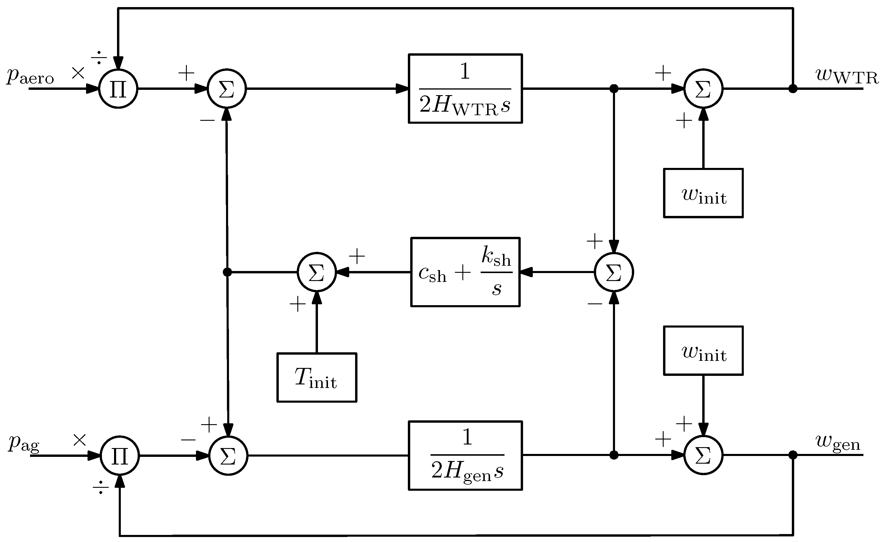
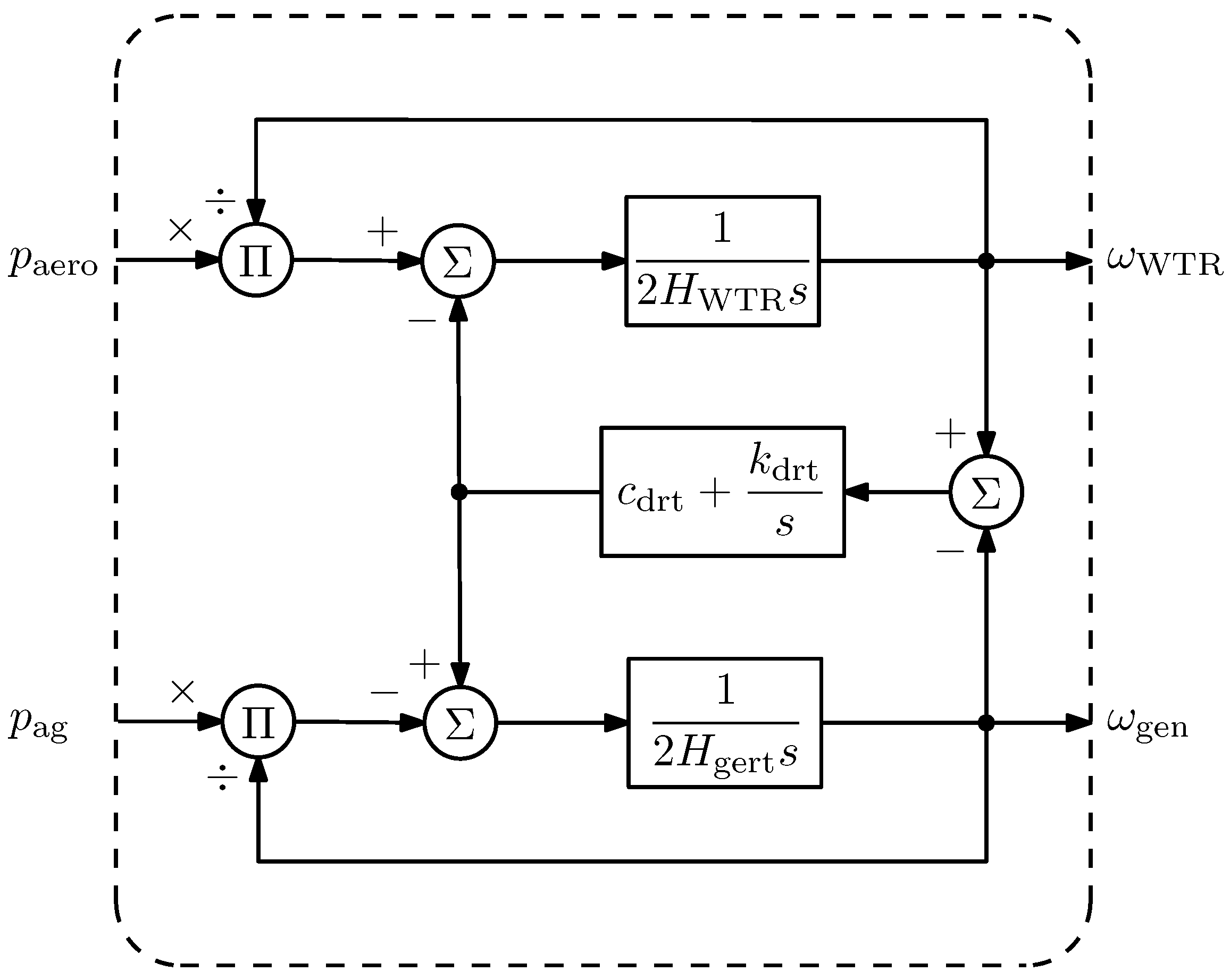
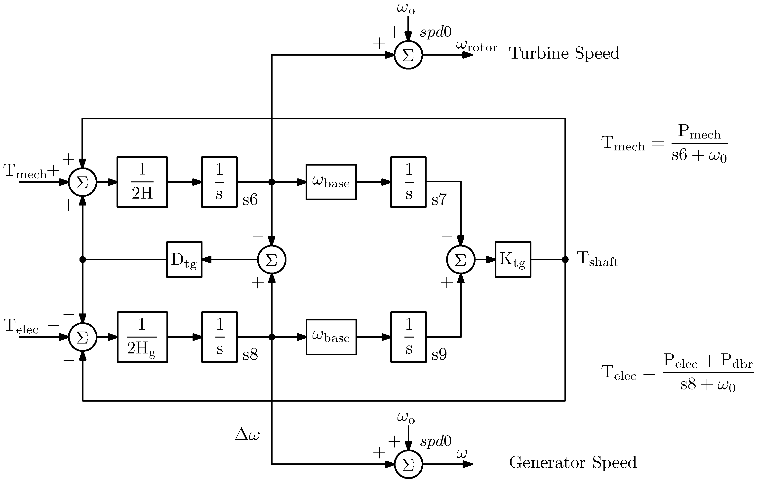
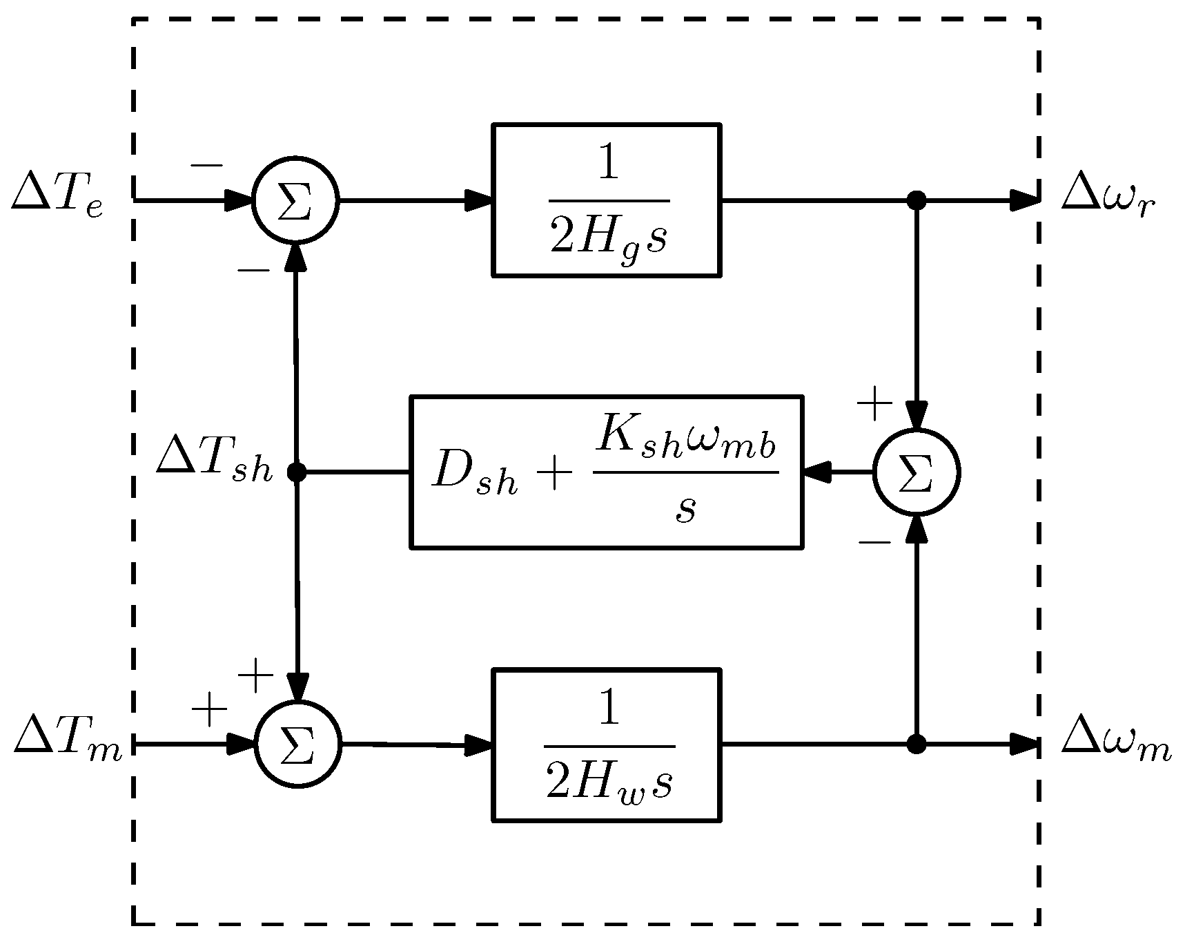
Furthermore, the pu equations for the two-mass drive train model that can be derived from the block diagrams shown in Figure 4 in [26] and Figure 21 in [27] are structurally different from those models that can be derived from either the block diagrams in Figures 4–10 in [28] or Figure 3 (Rotor Model) in [29]. Thus, comparison of results in different works is frequently hindered.

Figure 4 in [26], Figure 21 in [27], Figures 4–10 in [28] and Figure 3 (Rotor Model) in [29] have been reproduced here as a reference, see Figure 1, Figure 2, Figure 3 and Figure 4 in this work.

In regard to the dimensioning of base values, the base for the spring constant in [30] (p. 42) is expressed in $\mathrm{N}·\mathrm{m}/(\mathrm{rad}/\mathrm{s})$, whereas in [2] (p. 542), the base for the shaft stiffness, as it is also known, is expressed in $\mathrm{N}·\mathrm{m}/\mathrm{rad}$, with the latter being consistent with [31] (cf. [2] (p. 542) and [3]). Similarly, the per-unit shaft stiffness is reported to be expressed in different dimensions; for example, in [26], it is expressed in $\mathrm{pu}$, in [29], it is reported in $\mathrm{rad}$, whereas in [32], it is reported in $\mathrm{pu}/\mathrm{elec}.\mathrm{rad}$. Therefore, in the wind energy literature, there seems to be a clear issue regarding dimensional consistency.

Regarding order-of-magnitude inconsistencies, there are instances where pu parameters such as those corresponding to wind turbines of similar power ratings have values that are extremely different from each other. For example, in [26], the two-mass drive train shaft stiffness $k_{\mathrm{sh}}$ is equal to $150.0052\mathrm{pu}$, whereas in [24], shaft stiffness $k_s$ is equal to $0.6\mathrm{pu}$.

The main contribution of this work is to compute fully unambiguous and dimensionally homogeneous per-unit parameters of a two-mass drive train model for a set of representative traceable Reference Wind Turbines. We address the current modeling landscape, in which the absence of standardized per-unit drive train models and their associated parameters hampers effective benchmarking and limits the comparability of results across the literature.

This paper is structured as follows. Section 2 summarizes the per-unit conversion method which is later applied to the real parameter data for a two-mass model of a set of representative RWTs. In Section 3, expressions for the calculation of base quantities and expressions for the per-unit conversion are derived. In Section 4, the per-unit mathematical model, the corresponding block diagram, and the per-unit parameters of the two-mass drive train for the Reference Wind Turbines are presented. In addition, Section 4 contains a discussion about the per-unit conversion method based on the Bond Graph methodology and its application. Finally, in Section 5, the main conclusions are drawn about the importance of the calculated per-unit data in the context of simulation of wind farms.

2. Materials and Methods

2.1. Bond Graph Methodology

The Bond Graph is a graphical methodology that describes the interchange of energy in physical dynamic systems [4]. The BG methodology is a multi-domain approach for modeling dynamic systems; it employs the power conjugate variables effort e and flow f to describe the instantaneous flow of energy between different components of the system regardless of the domain they belong to (see

Table 1. Energy domains and their corresponding power conjugate variables (effort and flow) [4].

Energy Domain	Effort $\left(\mathit{e}\right)$	Flow $\left(\mathit{f}\right)$
Translational mechanics	Force (F)	Speed (v)
Rotational mechanics	Angular momentum (M)	Angular speed ($\omega$)
Electric domain	Voltage (u)	Current (i)
Magnetic domain	Magnetomotive force (V)	Magnetic flux rate ($\dot{\Phi }$)
Hydraulic domain	Total pressure ($\mathrm{p}$)	Volume flow (Q)
Thermo-dynamic	Temperature (T)	Entropy flow ($\dot{S}$)
Chemical domain	Chemical potential ($\mu$)	Molar flow ($\dot{N}$)

for a physical interpretation of effort and flow for different energy domains). Standard nomenclature, for generic variables and generic parameters regardless of the energy domain, is shown in

Table 2. Nomenclature for generic variables and generic parameters regardless of the energy domain [3,4].

Variable/Parameter	Symbol
Effort	e
Flow	f
Power	P
Generalized displacement	q
Generalized momentum	p
Energy	E
Resistance	R
Inertia	I
Capacitance	C

[3,4].

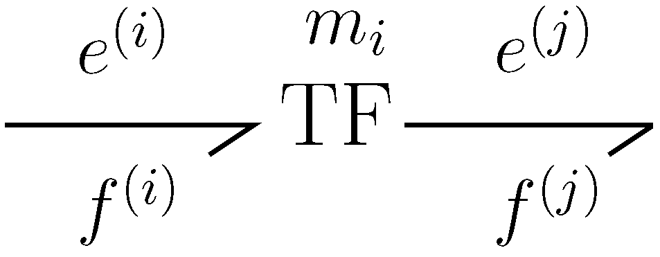
A 2-port TF element is a power-conserving BG element; it is denoted by using the TF symbol (see Figure 5).

The constitutive equation of the transformer element TF, relating effort e and flow f, is given by

$$\left\{\begin{array}{ccc}\hfill f^{\left(j\right)}& =& m_i{f}^{\left(i\right)}\hfill \\ \hfill m_i{e}^{\left(j\right)}& =& e^{\left(i\right)}\hfill \end{array}\right.$$

(11)

where $m_i$ is the TF element modulus; a quantity referred to the primary stage of the TF element (inwards-pointing half arrow) is identified with the superscript $\left(i\right)$; similarly, a quantity referred to the secondary stage of a TF element (outwards-pointing half arrow) is identified with the superscript $\left(j\right)$, see Figure 5.

Given the power-conserving property of the TF element, the equation

$$P_b=e_b^{\left(i\right)}{f}_b^{\left(i\right)}$$

(12)

relates the base effort, flow, and power for every stage (i) of a Weighted Junction Structure (WJS) BG with simple loops, where a TF element couples every pair of stages (i) and (j) of the BG [3].

The reader is referred to [4,5,6] and references therein for additional information regarding the BG methodology.

2.2. Base Quantities Propagation

Using the methodology proposed in [3], effort, flow, generalized displacement, and generalized momentum base quantities are propagated through the 2-port TF element using

$$\left\{\begin{array}{ll}\hfill f_b^{\left(j\right)}& =m_i{f}_b^{\left(i\right)}\\ \hfill m_i{e}_b^{\left(j\right)}& =e_b^{\left(i\right)}\end{array}\right.$$

(13)

$$\left\{\begin{array}{ll}\hfill q_b^{\left(j\right)}& =m_i{q}_b^{\left(i\right)}\\ \hfill m_i{p}_b^{\left(j\right)}& =p_b^{\left(i\right)}\end{array}\right.$$

(14)

where $m_i\in {\mathbb{R}}^{+}$ denotes the modulus of the TF element, considered a parameter with a constant value.

Using Equations (13) and (14) yields

$${\displaystyle \frac{q_b}{f_b}}={\displaystyle \frac{q_b^{\left(i\right)}}{f_b^{\left(i\right)}}}={\displaystyle \frac{q_b^{\left(j\right)}}{f_b^{\left(j\right)}}}$$

(15)

Furthermore, in each and every stage of the BG, Equations

$$E_b:=P_b$$

(16)

$$R_b{f}_b=e_b$$

(17)

$$p_b:=e_b$$

(18)

$$q_b=C_b{e}_b$$

(19)

can be used to calculate energy, resistance, generalized momentum, and capacitance base quantities [3].

Finally,

$$\begin{array}{cc}\hfill \hat{R}& ={\displaystyle \frac{f_b}{e_b}}R={\displaystyle \frac{R}{R_b}}=\overline{R}\hfill \end{array}$$

(20)

$$\begin{array}{cc}\hfill \hat{I}& ={\displaystyle \frac{f_b}{e_b}}I={\displaystyle \frac{I}{R_b}}=2H\hfill \end{array}$$

(21)

$$\begin{array}{cc}\hfill \hat{C}& ={\displaystyle \frac{e_b}{f_b}}C=R_{b}C={\displaystyle \frac{q_b}{f_b}}\overline{C}\hfill \end{array}$$

(22)

correspond to the equivalent per-unit resistance, inertia, and capacitance of the 1-port R, I, and C elements with linear characteristics, which can be used in the per-unitized BG [3].

These equations can be used to define pu 1-junction, 0-junction, Se, Sf, and TF elements that retain their constitutive equations.

The pu-equivalent 1-port R BG element with linear characteristics has the following equation with resistance causality

$$\overline{R}\overline{f}=\overline{e}$$

(23)

The pu-equivalent 1-port I and C BG elements with linear characteristics have the following equations with differential causality [4]:

$$\begin{array}{cc}\hfill \hat{p}& ={\displaystyle \frac{p}{e_b}}={\int }_{-\infty }^t\overline{e}\mathrm{d}\tau \hfill \end{array}$$

(24)

$$\begin{array}{cc}\hfill \hat{p}& =\hat{I}\overline{f}=2H\overline{f}\hfill \end{array}$$

(25)

$$\begin{array}{cc}\hfill \hat{I}{\displaystyle \frac{\mathrm{d}\overline{f}}{\mathrm{d}t}}& =\overline{e}\hfill \end{array}$$

(26)

$$\begin{array}{cc}\hfill \overline{q}& ={\displaystyle \frac{f_b}{q_b}}{\int }_{-\infty }^t\overline{f}\mathrm{d}\tau \hfill \end{array}$$

(27)

$$\begin{array}{cc}\hfill \overline{q}& ={\displaystyle \frac{f_b}{q_b}}\hat{C}\overline{e}=\overline{C}\overline{e}\hfill \end{array}$$

(28)

$$\begin{array}{cc}\hfill \hat{C}{\displaystyle \frac{\mathrm{d}\overline{e}}{\mathrm{d}t}}& =\overline{f}\hfill \end{array}$$

(29)

where the inertia constant H is defined by

$$H:={\displaystyle \frac{1}{2}}I{\displaystyle \frac{f_b}{e_b}}$$

(30)

It is notable that Equations (14), (24) and (27) are important definitions in the context of Bond Graphs, and these may allow for an alternative selection of state variables.

Definition 1 

(Base quantities’ propagation trajectory). A base quantities’ propagation trajectory is a line of flow contained in the junction structure of a Bond Graph with a WJS that goes through the $\{0,1,\mathrm{TF}\}$ nodes and that is ancillary during the process of sequential assignment of base quantities associated with the propagation of the base quantities throughout the Bond Graph. These trajectories carry the base quantities $e_b,f_b,p_b,q_b$, and $P_b$. The beginning of a base quantities’ propagation trajectory is on any stage of the Bond Graph and its termination is at the port of the various graph elements or on the bonds where base quantity assignment conflicts arise.

Base quantities’ propagation trajectories serve as visual support during the realization of the base quantities’ propagation throughout the Bond Graph.

A propagation trajectory can be oriented arbitrarily; nonetheless, it is subject to the following restrictions:

• When it goes through a TF element, base quantities that are propagated to the primary side (i) or secondary side (j) of this element satisfy Equations (13) and (14).
• On the same Bond Graph, propagation trajectories with different base power $P_b$ or different $f_b/q_b$ ratios cannot coexist.
• Conjoined propagation trajectories propagate the same base quantities.

The reader may consult additional information regarding the BG methodology in [4,5,6] and references therein.

2.3. Converting Per-Unit Values When Base Values Are Changed

Consider Equation (12). If, at stage (0), the flow base value $f_b^{\left(0\right)}$ is defined, it follows that the corresponding effort base value $e_b^{\left(0\right)}$ must satisfy the following condition.

$$P_b=e_b^{\left(0\right)}{f}_b^{\left(0\right)}$$

(31)

It is known that, for convenience, all per-unit variables and parameters may be referred to the stage (i) where the generalized displacement base value $q_b^{\left(i\right)}$ is set to 1, which, in wind energy generation systems, typically corresponds to the electrical stage (0) where $q_b^{\left(0\right)}\equiv {\theta }_b^{\left(0\right)}=1\mathrm{rad}$ [3]. For simplicity, we drop the use of superscript (0). Thus, on stage (0), equivalent per-unit parameters in Equations (20)–(22) may be converted from the old base values $\{e_{b,x},f_{b,x},P_{b,x}\}$ to the new base values $\{e_{b,y},f_{b,y},P_{b,y}=P_{b,x}\}$ using:

$$\begin{array}{c}\hfill {\hat{R}}_y={\overline{R}}_y={\displaystyle \frac{R_{b,x}}{R_{b,y}}}{\overline{R}}_x={\displaystyle \frac{f_{b,y}}{e_{b,y}}}{\displaystyle \frac{e_{b,x}}{f_{b,x}}}{\hat{R}}_x\end{array}$$

(32)

$$\begin{array}{c}\hfill {\hat{I}}_y=2H_y={\displaystyle \frac{R_{b,x}}{R_{b,y}}}{\hat{I}}_x=2{\displaystyle \frac{f_{b,y}}{e_{b,y}}}{\displaystyle \frac{e_{b,x}}{f_{b,x}}}{H}_x\end{array}$$

(33)

$$\begin{array}{c}\hfill {\hat{C}}_y={\displaystyle \frac{q_b}{f_{b,y}}}{\overline{C}}_y={\displaystyle \frac{R_{b,y}}{R_{b,x}}}{\hat{C}}_x={\displaystyle \frac{R_{b,y}}{R_{b,x}}}{\displaystyle \frac{q_b}{f_{b,x}}}{\overline{C}}_x\end{array}$$

(34)

where subscripts x and y on the equivalent per-unit parameters correspond to the respective base values to which they refer. This conversion procedure is useful when the power base value $P_b$ is kept unchanged, i.e., $P_b=P_{b,x}=P_{b,y}$, and the flow base value $f_b$ to which per-unit quantities are referred is changed from $f_{b,x}$ to $f_{b,y}$.

2.4. Bond Graph in Real Quantities for the Two-Mass Drive Train Model

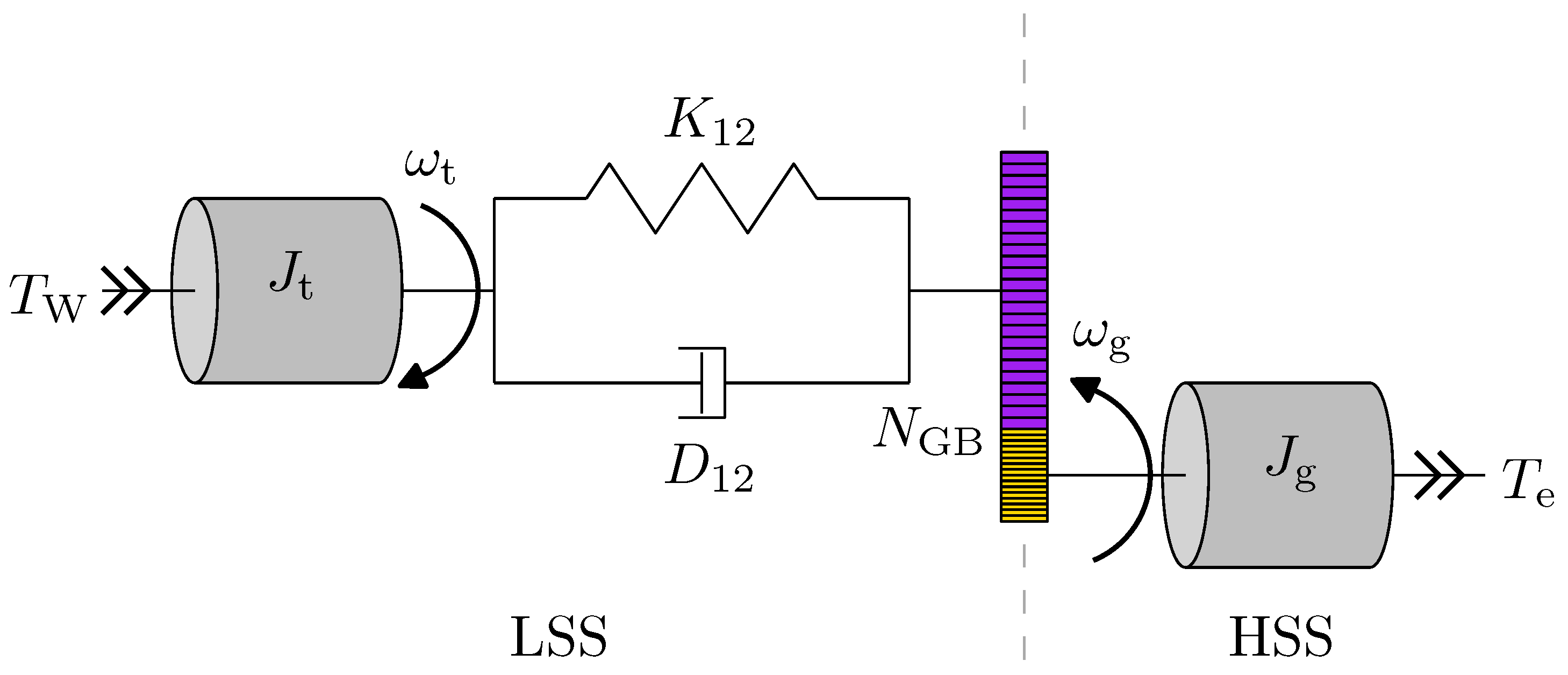
The wind turbine drive train can be modeled through the rotating mass system shown in Figure 6, where ${\omega }_{\mathrm{t}}$ is the rotor axis angular speed of the wind turbine and ${\omega }_{\mathrm{g}}$ is the generator axis angular speed, respectively, in $\mathrm{rad}/\mathrm{s}$. ${\theta }_{\mathrm{t}}$ is the angular position of the rotor axis and ${\theta }_{\mathrm{g}}$ is the angular position of the generator axis, respectively, in $\mathrm{rad}$. $T_{\mathrm{W}}$ is the wind turbine acceleration torque, $T_{\mathrm{e}}$ is the electric torque of the machine in generator convention, and $T_{K_{12}}$ is the torsionally elastic torque component of the shaft related to ${\theta }_{\mathrm{t}}$ and ${\theta }_{\mathrm{g}}$ by $T_{K_{12}}=K_{12}({\theta }_{\mathrm{t}}-{\theta }_{\mathrm{g}}/N_{\mathrm{GB}})$, respectively, in $\mathrm{N}·\mathrm{m}$. The remaining parameters are described in

Table 3. Nomenclature and units.

Parameter	Units	Description
$P_b$	$\mathrm{MW}$	Nominal power, base power
$N_{\mathrm{GB}}$	1	Gear ratio
$n_p$	-	Number of poles
$J_{\mathrm{g}}$	$\mathrm{kg}·{\mathrm{m}}^2$	Generator inertia
$K_{12}$	$\mathrm{N}·\mathrm{m}/\mathrm{rad}$	LSS torsion resistance coefficient
$D_{12}$	$\mathrm{N}·\mathrm{m}·\mathrm{s}/\mathrm{rad}$	LSS damping coefficient
$J_{\mathrm{H}}$	$\mathrm{kg}·{\mathrm{m}}^2$	Hub inertia
$J_{\mathrm{HB}}$	$\mathrm{kg}·{\mathrm{m}}^2$	Blade pitch angle bearings inertia about the LSS
$J_{\mathrm{H}}^{\prime }$	$\mathrm{kg}·{\mathrm{m}}^2$	Total hub inertia
$J_{\mathrm{B}}$	$\mathrm{kg}·{\mathrm{m}}^2$	Blade inertia about the LSS
$J_{3\mathrm{B}}$	$\mathrm{kg}·{\mathrm{m}}^2$	Total blade inertia (three blades)
$J_{\mathrm{t}}$	$\mathrm{kg}·{\mathrm{m}}^2$	Rotor total inertia
${\omega }_b$	$\mathrm{rad}/\mathrm{s}$	Base angular speed
$H_{\mathrm{g}}$	s	Generator inertia
${\overline{K}}_{12}$	1	Torsion resistance coefficient
${\hat{K}}_{12}$	${\mathrm{s}}^{-1}$	Torsion resistance coefficient
${\overline{D}}_{12}$	1	Damping coefficient
$H_{\mathrm{t}}$	$\mathrm{s}$	Rotor total inertia

. In Figure 6, the high-speed and low-speed sides of the drive train are indicated using the labels HSS and LSS. Given its sufficient fidelity to the representation of the drive train dynamics, the two-mass dynamic model is typically used to carry out transitory response studies of wind energy systems [18,19,20].

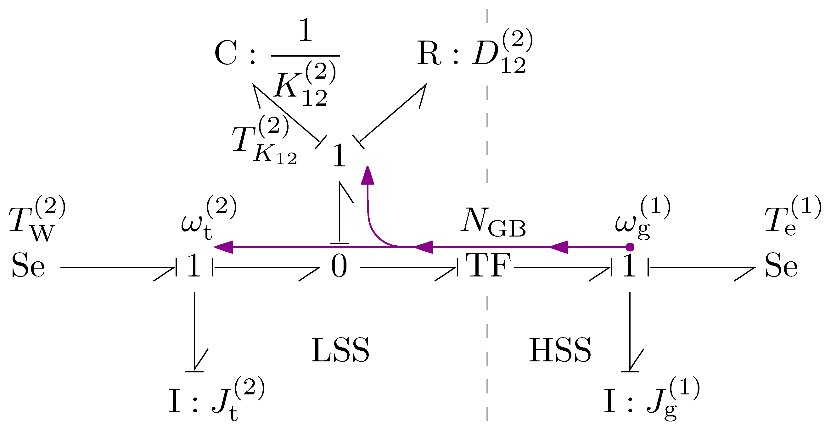
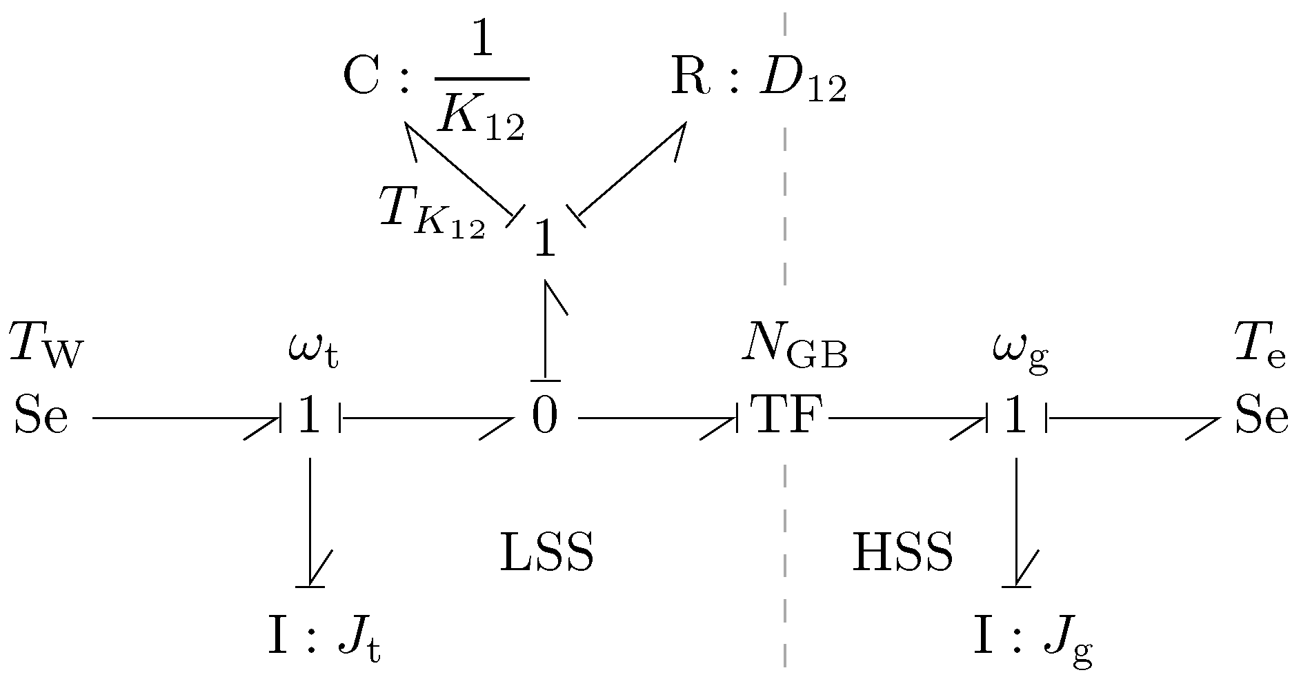
The Bond Graph model that corresponds with Figure 6 is shown in Figure 7 [5]. This Bond Graph model has already been causally completed, choosing integral causality as the preferred causality [4].

2.4.1. Mathematical Model in Real Quantities

The mathematical model in real quantities, derived from the two-mass drive train Bond Graph shown in Figure 7, was obtained manually following the procedure for manual derivation of equations from causal Bond Graphs (see [4,6]).

$$\left\{\begin{array}{ccc}\hfill {\displaystyle \frac{\mathrm{d}{T}_{K_{12}}}{\mathrm{d}t}}& =& K_{12}\left({\omega }_{\mathrm{t}}-{\displaystyle \frac{1}{N_{\mathrm{GB}}}}{\omega }_{\mathrm{g}}\right)\hfill \\ \hfill {\displaystyle \frac{\mathrm{d}{\omega }_{\mathrm{t}}}{\mathrm{d}t}}& =& {\displaystyle \frac{1}{J_{\mathrm{t}}}}\left(T_{\mathrm{W}}-T_{K_{12}}-D_{12}\left({\omega }_{\mathrm{t}}-{\displaystyle \frac{1}{N_{\mathrm{GB}}}}{\omega }_{\mathrm{g}}\right)\right)\hfill \\ \hfill {\displaystyle \frac{\mathrm{d}{\omega }_{\mathrm{g}}}{\mathrm{d}t}}& =& {\displaystyle \frac{1}{J_{\mathrm{g}}}}\left(-T_{\mathrm{e}}+{\displaystyle \frac{1}{N_{\mathrm{GB}}}}\left(T_{K_{12}}+D_{12}\left({\omega }_{\mathrm{t}}-{\displaystyle \frac{1}{N_{\mathrm{GB}}}}{\omega }_{\mathrm{g}}\right)\right)\right)\hfill \end{array}\right.$$

(35)

2.4.2. Data in Real Quantities

Through an exhaustive review of the literature, it was found that there is a relative lack of real data for wind turbines modeled using the two-mass concept. Nonetheless, in

Table 4. Two-mass model data in [14].

Parameter	Value	Units
$P_b$	5	$\mathrm{MW}$
$N_{\mathrm{GB}}$	$86.39$	1
$n_p$	6	-
$J_{\mathrm{g}}$	600	$\mathrm{kg}·{\mathrm{m}}^2$
$K_{12}$	$7.5\times {10}^8$	$\mathrm{N}·\mathrm{m}/\mathrm{rad}$
$D_{12}$	0	$\mathrm{N}·\mathrm{m}/(\mathrm{rad}/\mathrm{s})$
$J_{\mathrm{H}}$	110,000	$\mathrm{kg}·{\mathrm{m}}^2$
$J_{\mathrm{HB}}$	NaN	$\mathrm{kg}·{\mathrm{m}}^2$
$J_{\mathrm{H}}^{\prime }$	110,000	$\mathrm{kg}·{\mathrm{m}}^2$
$J_{\mathrm{B}}$	$7.381\times {10}^6$	$\mathrm{kg}·{\mathrm{m}}^2$
$J_{3\mathrm{B}}$	$2.2143\times {10}^7$	$\mathrm{kg}·{\mathrm{m}}^2$
$J_{\mathrm{t}}$	$2.2253\times {10}^7$	$\mathrm{kg}·{\mathrm{m}}^2$

Source: [14].

,

Table 5. Two-mass model data in [15].

Parameter	Value	Units
$P_b$	5	$\mathrm{MW}$
$N_{\mathrm{GB}}$	97	1
$n_p$	6	-
$J_{\mathrm{g}}$	$534.116$	$\mathrm{kg}·{\mathrm{m}}^2$
$K_{12}$	867,637,000	$\mathrm{N}·\mathrm{m}/\mathrm{rad}$
$D_{12}$	6,215,000	$\mathrm{N}·\mathrm{m}/(\mathrm{rad}/\mathrm{s})$
$J_{\mathrm{H}}$	115,926	$\mathrm{kg}·{\mathrm{m}}^2$
$J_{\mathrm{HB}}$	$\mathrm{NaN}$	$\mathrm{kg}·{\mathrm{m}}^2$
$J_{\mathrm{H}}^{\prime }$	115,926	$\mathrm{kg}·{\mathrm{m}}^2$
$J_{\mathrm{B}}$	11,776,047	$\mathrm{kg}·{\mathrm{m}}^2$
$J_{3\mathrm{B}}$	35,328,141	$\mathrm{kg}·{\mathrm{m}}^2$
$J_{\mathrm{t}}$	$3.5444067\times {10}^7$	$\mathrm{kg}·{\mathrm{m}}^2$

Source: [15].

,

Table 6. Two-mass model data in [16,17]; $750\mathrm{kW}$ wind turbine.

Parameter	Value	Units
$P_b$	$0.75$	$\mathrm{MW}$
$N_{\mathrm{GB}}$	$62.83185307$	1
$n_p$	4	-
$J_{\mathrm{g}}$	$16.651$	$\mathrm{kg}·{\mathrm{m}}^2$
$K_{12}$	129,646,445	$\mathrm{N}·\mathrm{m}/\mathrm{rad}$
$D_{12}$	278,494	$\mathrm{N}·\mathrm{m}/(\mathrm{rad}/\mathrm{s})$
$J_{\mathrm{H}}$	5161	$\mathrm{kg}·{\mathrm{m}}^2$
$J_{\mathrm{HB}}$	2324.2	$\mathrm{kg}·{\mathrm{m}}^2$
$J_{\mathrm{H}}^{\prime }$	7485.17321	$\mathrm{kg}·{\mathrm{m}}^2$
$J_{\mathrm{B}}$	180,640	$\mathrm{kg}·{\mathrm{m}}^2$
$J_{3\mathrm{B}}$	541,920	$\mathrm{kg}·{\mathrm{m}}^2$
$J_{\mathrm{t}}$	$5.494051732\times {10}^5$	$\mathrm{kg}·{\mathrm{m}}^2$

Source: [16,17].

,

Table 7. Two-mass model data in [16,17]; $1.5\mathrm{MW}$ wind turbine.

Parameter	Value	Units
$P_b$	$1.5$	$\mathrm{MW}$
$N_{\mathrm{GB}}$	$87.965$	1
$n_p$	4	-
$J_{\mathrm{g}}$	$56.442$	$\mathrm{kg}·{\mathrm{m}}^2$
$K_{12}$	483,129,640	$\mathrm{N}·\mathrm{m}/\mathrm{rad}$
$D_{12}$	1,355,794	$\mathrm{N}·\mathrm{m}/(\mathrm{rad}/\mathrm{s})$
$J_{\mathrm{H}}$	29,975	$\mathrm{kg}·{\mathrm{m}}^2$
$J_{\mathrm{HB}}$	12,500.2	$\mathrm{kg}·{\mathrm{m}}^2$
$J_{\mathrm{H}}^{\prime }$	42,475.20625	$\mathrm{kg}·{\mathrm{m}}^2$
$J_{\mathrm{B}}$	798,506	$\mathrm{kg}·{\mathrm{m}}^2$
$J_{3\mathrm{B}}$	2,395,518	$\mathrm{kg}·{\mathrm{m}}^2$
$J_{\mathrm{t}}$	$2.437993206\times {10}^6$	$\mathrm{kg}·{\mathrm{m}}^2$

Source: [16,17].

,

Table 8. Two-mass model data in [16,17]; $3\mathrm{MW}$ wind turbine.

Parameter	Value	Units
$P_b$	3	$\mathrm{MW}$
$N_{\mathrm{GB}}$	$124.4070691$	1
$n_p$	4	-
$J_{\mathrm{g}}$	$177.885$	$\mathrm{kg}·{\mathrm{m}}^2$
$K_{12}$	1,039,402,036	$\mathrm{N}-\mathrm{m}/\mathrm{rad}$
$D_{12}$	4,992,005	$\mathrm{N}-\mathrm{m}/(\mathrm{rad}/\mathrm{s})$
$J_{\mathrm{H}}$	197,987	$\mathrm{kg}·{\mathrm{m}}^2$
$J_{\mathrm{HB}}$	70,729.9	$\mathrm{kg}·{\mathrm{m}}^2$
$J_{\mathrm{H}}^{\prime }$	268,716.97303	$\mathrm{kg}·{\mathrm{m}}^2$
$J_{\mathrm{B}}$	5,012,212	$\mathrm{kg}·{\mathrm{m}}^2$
$J_{3\mathrm{B}}$	15,036,636	$\mathrm{kg}·{\mathrm{m}}^2$
$J_{\mathrm{t}}$	$1.530535297\times {10}^7$	$\mathrm{kg}·{\mathrm{m}}^2$

Source: [16,17].

and

Table 9. Two-mass model data in [16,17]; $5\mathrm{MW}$ wind turbine.

Parameter	Value	Units
$P_b$	5	$\mathrm{MW}$
$N_{\mathrm{GB}}$	$160.8495439$	1
$n_p$	4	-
$J_{\mathrm{g}}$	$438.855$	$\mathrm{kg}·{\mathrm{m}}^2$
$K_{12}$	2,300,693,020	$\mathrm{N}·\mathrm{m}/\mathrm{rad}$
$D_{12}$	14,909,175	$\mathrm{N}·\mathrm{m}/(\mathrm{rad}/\mathrm{s})$
$J_{\mathrm{H}}$	668,485	$\mathrm{kg}·{\mathrm{m}}^2$
$J_{\mathrm{HB}}$	255,550.6	$\mathrm{kg}·{\mathrm{m}}^2$
$J_{\mathrm{H}}^{\prime }$	924,035.57012	$\mathrm{kg}·{\mathrm{m}}^2$
$J_{\mathrm{B}}$	17,475,408	$\mathrm{kg}·{\mathrm{m}}^2$
$J_{3\mathrm{B}}$	52,426,224	$\mathrm{kg}·{\mathrm{m}}^2$
$J_{\mathrm{t}}$	$5.335025957\times {10}^7$	$\mathrm{kg}·{\mathrm{m}}^2$

Source: [16,17].

, open-access and readily verifiable datasets are presented, which are provided by the Risø National Laboratory [14] and National Renewable Energy Laboratory (NREL) [15,16,17]. Not all data shown in Table 4, Table 5, Table 6, Table 7, Table 8 and Table 9 can be found in the cited references; some were calculated using the modeling assumptions found in Section 2.4.3 corresponding with Method-2 for the order reduction of the drive train model, detailed in [30]. As mentioned in [13], RWTs have proven to be very useful for the research and technological community. The $5\mathrm{MW}$ NREL wind turbine [15], developed in 2005, is one of the most widely known RWTs [20,33]. The $5\mathrm{MW}$ NREL reference wind turbine was developed using a combination of commercial wind turbine data and parameters taken from other contemporary wind turbines [15].

2.4.3. Lumped Parameter Model

In order to fit the data shown in Table 4, Table 5, Table 6, Table 7, Table 8 and Table 9 for the two-mass model presented in Section 2.4, Method-2 was employed, as detailed in [30], for the order reduction of a six-mass horizontal-axis wind turbine model under the following modeling assumptions:

• It is assumed that the wind turbine blades are infinitely stiff. Also, it is assumed that all of the inertia moments about the blade root of each of the three blades, on the low-speed side, have the same magnitude, i.e., $J_{\mathrm{B}1}=J_{\mathrm{B}2}=J_{\mathrm{B}3}=J_{\mathrm{B}}$ [16,30]. Thus, the wind turbine can be considered to be a disk with a large radius and small thickness, having an evenly distributed mass, such that the total moment of inertia of the three blades is equal to the sum of the moments of inertia of each one blade, i.e., $J_{3\mathrm{B}}=J_{\mathrm{B}1}+J_{\mathrm{B}2}+J_{\mathrm{B}3}=3J_{\mathrm{B}}$ [30].
• It is considered that the rotating elements on the LSS which significantly contribute to the total inertia of the rotor are the hub, with inertia $J_{\mathrm{H}}$, and the bearings of the three blades, with inertia $J_{\mathrm{HB}}$. Thus, the total hub inertia $J_{\mathrm{H}}^{\prime }$ can be likened to that of a disk, and it can be calculated using $J_{\mathrm{H}}^{\prime }=J_{\mathrm{H}}+J_{\mathrm{HB}}$.
• The total rotor inertia $J_{\mathrm{t}}$, on the LSS, can be calculated under the assumption that the torsion resistance coefficient on the LSS referred to the HSS is smaller than that on the HSS [30]. Thus, the total rotor inertia can be calculated by adding the inertias of the wind turbine blades and hub equivalent disks, i.e., $J_{\mathrm{t}}=J_{3\mathrm{B}}+J_{\mathrm{H}}^{\prime }$.
• It is assumed that the generator inertia value $J_{\mathrm{g}}$ which is provided in the various datasheets conforms to the consideration that, with the HSS shaft being infinitely rigid, the elements with outstanding inertia values are the HSS shaft, couplings, and break disks, thus neglecting the value of the gearbox inertia.

3. Calculation

3.1. Pu Conversion

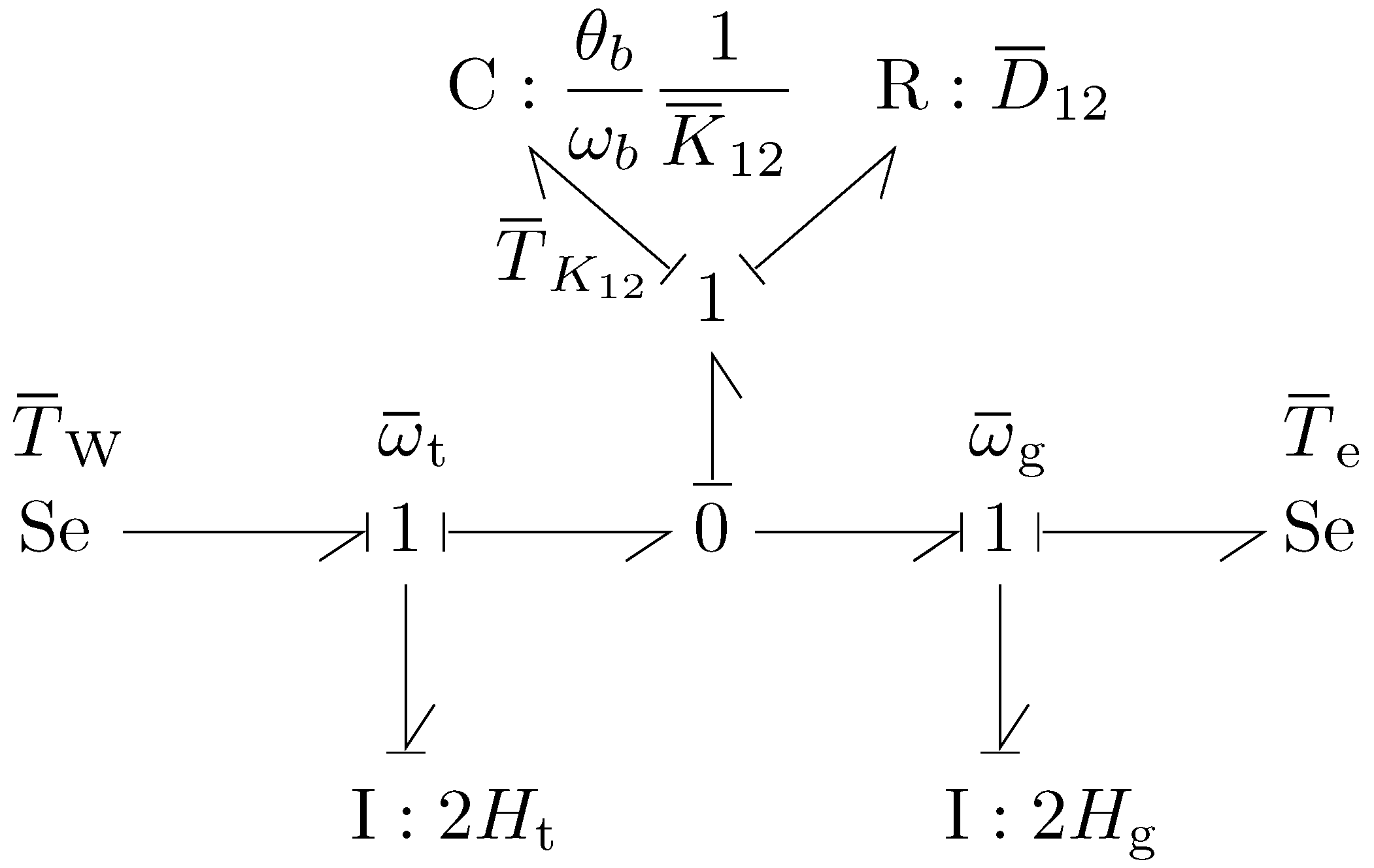
Per-unit parameter conversion based on the BG methodology was applied to calculate the two-mass drive train model parameters in pu. In order to carry out the conversion of the Bond Graph shown in Figure 7 to the pu system using the methodology described in [3], the propagation of the base quantities is performed through all of the Bond Graph stages following the propagation trajectories, as shown in Figure 8. In Figure 8, it can be noticed that variables and parameters associated with the base quantities of stage (i) have the superscript (i).

It can be observed that in the rotational mechanics energy domain, mechanical torque T corresponds with the effort variable e, angular velocity $\omega$ corresponds with the flow variable f, angular momentum L corresponds with the generalized momentum variable p, angular position $\theta$ corresponds with the generalized displacement q, damping coefficient D corresponds with resistance R, moment of inertia J corresponds with inertia I, and the reciprocal of the torsion resistance coefficient K corresponds with capacitance C, respectively, i.e., $e\equiv T$, $f\equiv \omega$, $p\equiv L$, $q\equiv \theta$, $R\equiv D$, $I\equiv J$, and $C\equiv 1/K$.

3.1.1. Definition of the Base Quantities

Stage (0)

Firstly, in Stage (0), base quantities $\{T_b^{\left(0\right)},{\omega }_b^{\left(0\right)},P_b^{\left(0\right)}\}$ are defined arbitrarily with $P_b=P_b^{\left(0\right)}=T_b^{\left(0\right)}{\omega }_b^{\left(0\right)}$, and ${\theta }_b^{\left(0\right)}$ is set to $1\mathrm{rad}$, i.e., ${\theta }_b^{\left(0\right)}:=1\mathrm{rad}$. Following this definition and using Equations (12)–(14) and (16)–(19), the remaining base quantities, i.e., $T_b:=P_b/{\omega }_b$, $E_b:=P_b$, $L_b:=T_b$, $D_b:=T_b/{\omega }_b$, and $C_b\equiv 1/K_b:={\theta }_b/T_b$, will be calculated from the base quantities ${\omega }_b^{\left(0\right)},P_b$, and ${\theta }_b^{\left(0\right)}$ in each stage of the BG.

Using Equations (12), (13), (17),and (19), it follows that:

$$T_b^{\left(0\right)}:={\displaystyle \frac{P_b}{{\omega }_b^{\left(0\right)}}}$$

(36)

$$D_b^{\left(0\right)}:={\displaystyle \frac{T_b^{\left(0\right)}}{{\omega }_b^{\left(0\right)}}}$$

(37)

$$C_b^{\left(0\right)}\equiv {\displaystyle \frac{1}{K_b^{\left(0\right)}}}:={\displaystyle \frac{{\theta }_b^{\left(0\right)}}{T_b^{\left(0\right)}}}$$

(38)

Stage (1)

In the sequel, the computation of base quantities ${\omega }_b^{\left(1\right)}$ and ${\theta }_b^{\left(1\right)}$ associated with Stage (1) is performed using the base quantities of Stage (0), following Equations (13) and (14).

Assuming that the base values of Stage (0) were defined on the electrical stage of an $n_p$-pole electric machine, e.g., $n_p=4$, it follows that the computation of the base quantities of Stage (1) can be calculated as

$$\begin{array}{cc}\hfill {\omega }_b^{\left(1\right)}& ={\displaystyle \frac{2}{n_p}}{\omega }_b^{\left(0\right)}\hfill \end{array}$$

(39)

$$\begin{array}{cc}\hfill {\theta }_b^{\left(1\right)}& ={\displaystyle \frac{2}{n_p}}{\theta }_b^{\left(0\right)}\hfill \end{array}$$

(40)

Also, using Equations (12), (13), (17), and (19), the following base values are obtained for Stage (1):

$$\begin{array}{c}{T}_b^{\left(1\right)}:={\displaystyle \frac{P_b}{{\omega }_b^{\left(1\right)}}}\hfill \end{array}$$

(41)

$$\begin{array}{c}{D}_b^{\left(1\right)}:={\displaystyle \frac{T_b^{\left(1\right)}}{{\omega }_b^{\left(1\right)}}}\hfill \end{array}$$

(42)

$$\begin{array}{c}{C}_b^{\left(1\right)}\equiv {\displaystyle \frac{1}{K_b^{\left(1\right)}}}:={\displaystyle \frac{{\theta }_b^{\left(1\right)}}{T_b^{\left(1\right)}}}\hfill \end{array}$$

(43)

Stage (2)

Next, the computation of the base quantities ${\omega }_b^{\left(2\right)}$ and ${\theta }_b^{\left(2\right)}$ associated with Stage (2) is performed using the base quantities of Stage (1), following Equations (13) and (14). In these equations, the base quantities of the primary and secondary side of the TF:$m_i$ element have the associated superscripts (i) and (j), respectively, as shown in Figure 5.

Therefore, by observing that in Figure 8, the base quantities of Stage (1) are propagated from the secondary side, i.e., Stage (j), to the primary side of the TF:$N_{\mathrm{GB}}$ element, where the base quantities of Stage (2) are found, i.e., Stage (i), it follows that the computation of the base quantities of Stage (2) can be performed using:

$$\begin{array}{c}{\omega }_b^{\left(2\right)}={\displaystyle \frac{1}{N_{\mathrm{GB}}}}{\omega }_b^{\left(1\right)}\hfill \end{array}$$

(44)

$$\begin{array}{c}{\theta }_b^{\left(2\right)}={\displaystyle \frac{1}{N_{\mathrm{GB}}}}{\theta }_b^{\left(1\right)}\hfill \end{array}$$

(45)

Furthermore, using Equations (12), (13), (17) and (19), the following base values are obtained for Stage (2):

$$\begin{array}{c}\hfill T_b^{\left(2\right)}:={\displaystyle \frac{P_b}{{\omega }_b^{\left(2\right)}}}\end{array}$$

(46)

$$\begin{array}{c}\hfill D_b^{\left(2\right)}:={\displaystyle \frac{T_b^{\left(2\right)}}{{\omega }_b^{\left(2\right)}}}\end{array}$$

(47)

$$\begin{array}{c}\hfill C_b^{\left(2\right)}\equiv {\displaystyle \frac{1}{K_b^{\left(2\right)}}}:={\displaystyle \frac{{\theta }_b^{\left(2\right)}}{T_b^{\left(2\right)}}}\end{array}$$

(48)

To perform the conversion of the two-mass drive train BG model shown in Figure 8 to the per-unit system, the per-unit transformation (1) is employed reiteratively, and Equations (15), (20)–(22) and (30) are used to calculate the values of equivalent resistances, inertias, and capacitances of the BG in the per-unit system.

3.1.2. Pu Conversion of Variables and Parameters

For the BG shown in Figure 8, equivalent per-unit variables and parameters are calculated substituting the appropriate base values.

Stage (1)

$$\begin{array}{c}\hfill {\overline{T}}_{\mathrm{e}}={\displaystyle \frac{T_{\mathrm{e}}}{T_b^{\left(1\right)}}}\end{array}$$

(49)

$$\begin{array}{c}\hfill {\overline{\omega }}_{\mathrm{g}}={\displaystyle \frac{{\omega }_{\mathrm{g}}}{{\omega }_b^{\left(1\right)}}}\end{array}$$

(50)

$$\begin{array}{c}\hfill {\hat{I}}_{\mathrm{g}}=2H_{\mathrm{g}}={\displaystyle \frac{{\omega }_b^{\left(1\right)}}{T_b^{\left(1\right)}}}{J}_{\mathrm{g}}\end{array}$$

(51)

Stage (2)

$$\begin{array}{c}\hfill {\overline{T}}_{\mathrm{W}}={\displaystyle \frac{T_{\mathrm{W}}}{T_b^{\left(2\right)}}}\end{array}$$

(52)

$$\begin{array}{c}\hfill {\overline{T}}_{K_{12}}={\displaystyle \frac{T_{K_{12}}}{T_b^{\left(2\right)}}}\end{array}$$

(53)

$$\begin{array}{c}\hfill {\overline{\omega }}_{\mathrm{t}}={\displaystyle \frac{{\omega }_{\mathrm{t}}}{{\omega }_b^{\left(2\right)}}}\end{array}$$

(54)

$$\begin{array}{c}\hfill {\overline{D}}_{12}={\displaystyle \frac{D_{12}}{D_b^{\left(2\right)}}}\end{array}$$

(55)

$$\begin{array}{c}\hfill {\hat{I}}_{\mathrm{t}}=2H_{\mathrm{t}}={\displaystyle \frac{{\omega }_b^{\left(2\right)}}{T_b^{\left(2\right)}}}{J}_{\mathrm{t}}\end{array}$$

(56)

$$\begin{array}{c}\hfill {\overline{K}}_{12}={\displaystyle \frac{K_{12}}{K_b^{\left(2\right)}}}\end{array}$$

(57)

$$\begin{array}{c}\hfill {\hat{C}}_{12}={\displaystyle \frac{1}{{\hat{K}}_{12}}}={\displaystyle \frac{T_b^{\left(2\right)}}{{\omega }_b^{\left(2\right)}}}{\displaystyle \frac{1}{K_{12}}}={\displaystyle \frac{{\theta }_b}{{\omega }_b}}{\displaystyle \frac{1}{{\overline{K}}_{12}}}\end{array}$$

(58)

In summary, for this system defined in the rotational mechanics energy domain, the pu parameters that will be employed in the Bond Graph in the per-unit system are:

$$\begin{array}{c}\hfill \hat{R}=\overline{R}\equiv \overline{D}\end{array}$$

(59)

$$\begin{array}{c}\hfill \hat{I}=2H\end{array}$$

(60)

$$\begin{array}{c}\hfill \hat{C}\equiv {\displaystyle \frac{{\theta }_b}{{\omega }_b}}{\displaystyle \frac{1}{\overline{K}}}={\displaystyle \frac{1}{\hat{K}}}\end{array}$$

(61)

The appropriate values of variables and parameters are calculated following Equations (49)–(58), and the resulting values are substituted in the per-unit system Bond Graph that is shown in Figure 9.

4. Results and Discussion

4.1. Per-Unit System Bond Graph for the Two-Mass Drive Train Model

The result of the conversion of the two-mass drive train Bond Graph model from Section 2.4 is shown in Figure 9. In Figure 9, the reduction in the number of TF elements is notable. This is one of the key advantages of the pu system.

4.1.1. Per-Unit Mathematical Model

By applying the procedure for manual derivation of equations from causal BGs to the two-mass drive train Bond Graph in pu shown in Figure 9, the following per-unit mathematical model is obtained (see [4,6]).

$$\left\{\begin{array}{ccc}\hfill {\displaystyle \frac{\mathrm{d}{\overline{T}}_{K_{12}}}{\mathrm{d}t}}& =& {\omega }_b{\overline{K}}_{12}\left({\overline{\omega }}_{\mathrm{t}}-{\overline{\omega }}_{\mathrm{g}}\right)\hfill \\ \hfill {\displaystyle \frac{\mathrm{d}{\overline{\omega }}_{\mathrm{t}}}{\mathrm{d}t}}& =& {\displaystyle \frac{1}{2H_{\mathrm{t}}}}\left({\overline{T}}_{\mathrm{W}}-{\overline{T}}_{K_{12}}-{\overline{D}}_{12}\left({\overline{\omega }}_{\mathrm{t}}-{\overline{\omega }}_{\mathrm{g}}\right)\right)\hfill \\ \hfill {\displaystyle \frac{\mathrm{d}{\overline{\omega }}_{\mathrm{g}}}{\mathrm{d}t}}& =& {\displaystyle \frac{1}{2H_{\mathrm{g}}}}\left(-{\overline{T}}_{\mathrm{e}}+{\overline{T}}_{K_{12}}+{\overline{D}}_{12}\left({\overline{\omega }}_{\mathrm{t}}-{\overline{\omega }}_{\mathrm{g}}\right)\right)\hfill \end{array}\right.$$

(62)

with ${\omega }_b={\omega }_b^{\left(0\right)}$.

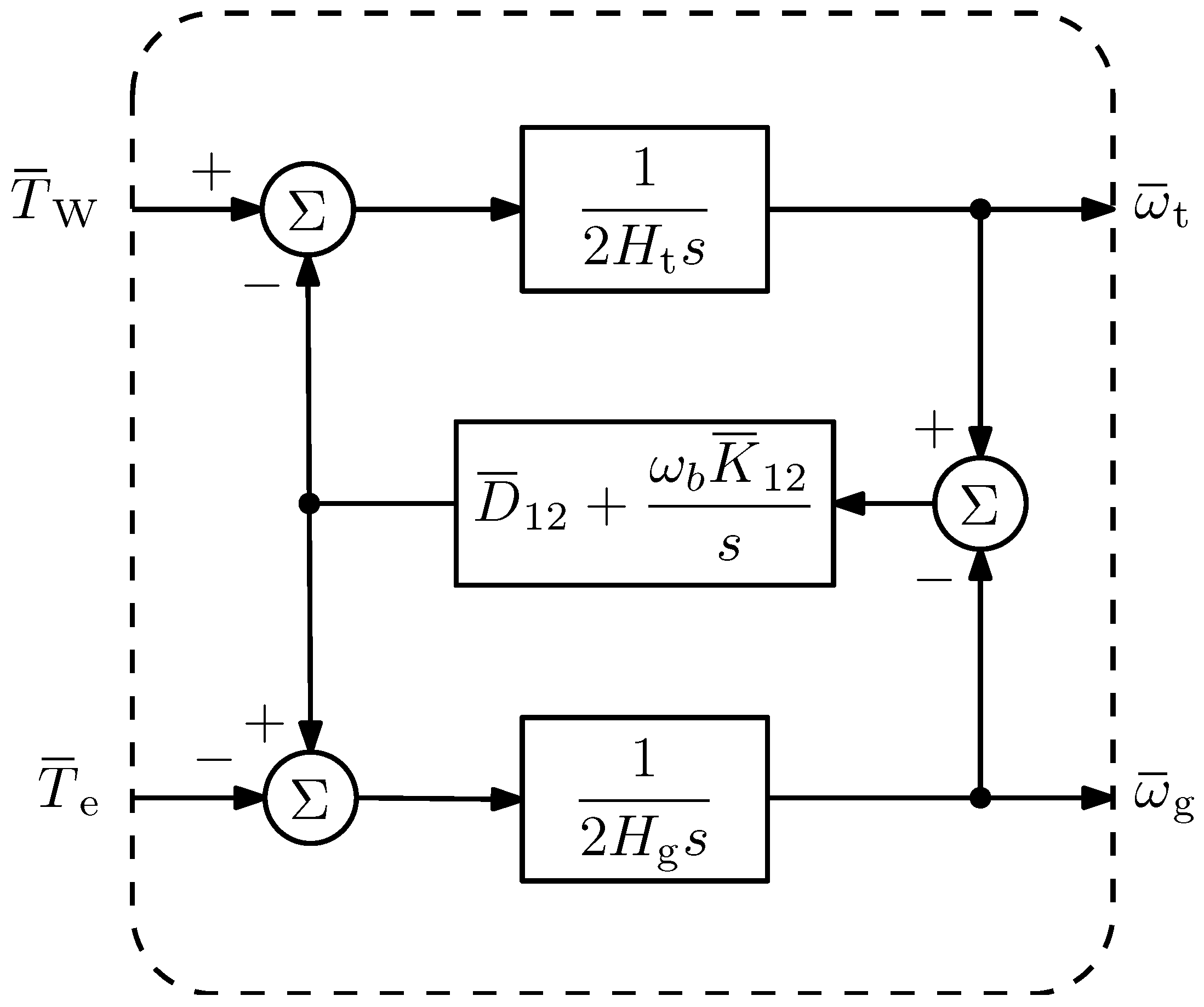
The block diagram model shown in Figure 10 can be derived from Equation (62). Notice that it features the product ${\omega }_b{\overline{K}}_{12}$ which is notably absent in [26,27] but present in [28,29].

Comparing the two-mass wind turbine drive train model shown in Figure 10 with those in Figure 2, Figure 3 and Figure 4 [27,28,29], it is noted that:

• The methodology presented in this work may be used to systematically produce mathematical models which are consistent with some of those models that can be found in the literature.
• The notation employed in this work enables the explicit univocal relationship of the parameters and variables in the pu system with those corresponding to the mathematical model in real quantities; therefore, it is less prone to producing human error [2].
• The pu conversion procedure, which employs the Bond Graph methodology, enables the production of datasets in the pu system based on datasets in real quantities, which, in turn, allows for the correct dimensioning of the dynamics of the wind turbines for various stability studies.
• Given the physical nature of electromechanical systems, the Bond Graph methodology facilitates an intermediate modeling stage for design, simulation, and control processes. Within this framework, mathematical expressions analogous to physical laws—derived from per-unit bond graphs (see [3])—provide a rigorous basis for evaluating the consistency and relevance of the data.

4.1.2. Data in Pu

For the two-mass drive train Bond Graph model shown in Figure 7, the result of applying the per-unit system conversion procedure described in Section 3.1 to the data contained in Table 4, Table 5, Table 6, Table 7, Table 8 and Table 9 can be found in

Table 10. Two-mass model data in [14] converted to pu.

Parameter	Value	Units
$P_b$	5	$\mathrm{MW}$
${\omega }_b$	$2\pi 60$	$\mathrm{rad}/\mathrm{s}$
$H_{\mathrm{g}}$	$0.947482023$	$\mathrm{s}$
${\overline{K}}_{12}$	$0.841885288$	1
${\hat{K}}_{12}$	$317.3832764$	${\mathrm{s}}^{-1}$
${\overline{D}}_{12}$	0	1
$H_{\mathrm{t}}$	$4.707851933$	$\mathrm{s}$

,

Table 11. Two-mass model data in [15] converted to pu with $5\mathrm{MW}$ nominal power.

Parameter	Value	Units
$P_b$	5	$\mathrm{MW}$
${\omega }_b$	$2\pi 60$	$\mathrm{rad}/\mathrm{s}$
$H_{\mathrm{g}}$	$0.84344218$	$\mathrm{s}$
${\overline{K}}_{12}$	$0.77252617$	1
${\hat{K}}_{12}$	$291.2355049$	${\mathrm{s}}^{-1}$
${\overline{D}}_{12}$	$2.086158915$	1
$H_{\mathrm{t}}$	$5.948669056$	$\mathrm{s}$

,

Table 12. Two-mass model data in [16,17]—$750\mathrm{kW}$ turbine converted to pu.

Parameter	Value	Units
$P_b$	750	$\mathrm{kW}$
${\omega }_b$	$2\pi 60$	$\mathrm{rad}/\mathrm{s}$
$H_{\mathrm{g}}$	$0.394413079$	$\mathrm{s}$
${\overline{K}}_{12}$	$4.126774513$	1
${\hat{K}}_{12}$	$1555.757339$	${\mathrm{s}}^{-1}$
${\overline{D}}_{12}$	$3.341933464$	1
$H_{\mathrm{t}}$	$3.296431039$	$\mathrm{s}$

,

Table 13. Two-mass model data in [16,17]—$1.5\mathrm{MW}$ turbine converted to pu.

Parameter	Value	Units
$P_b$	$1.5$	$\mathrm{MW}$
${\omega }_b$	$2\pi 60$	$\mathrm{rad}/\mathrm{s}$
$H_{\mathrm{g}}$	$0.668472254$	$\mathrm{s}$
${\overline{K}}_{12}$	$3.923049036$	1
${\hat{K}}_{12}$	$1478.954644$	${\mathrm{s}}^{-1}$
${\overline{D}}_{12}$	$4.150351512$	1
$H_{\mathrm{t}}$	$3.731587834$	$\mathrm{s}$

,

Table 14. Two-mass model data in [16,17]—$3\mathrm{MW}$ turbine converted to pu.

Parameter	Value	Units
$P_b$	3	$\mathrm{MW}$
${\omega }_b$	$2\pi 60$	$\mathrm{rad}/\mathrm{s}$
$H_{\mathrm{g}}$	$1.053392747$	$\mathrm{s}$
${\overline{K}}_{12}$	$2.109809865$	1
${\hat{K}}_{12}$	$795.3795807$	${\mathrm{s}}^{-1}$
${\overline{D}}_{12}$	$3.820022192$	$\mathrm{s}$
$H_{\mathrm{t}}$	$5.856042613$	$\mathrm{s}$

and

Table 15. Two-mass model data in [16,17]—$5\mathrm{MW}$ turbine converted to pu.

Parameter	Value	Units
$P_b$	5	$\mathrm{MW}$
${\omega }_b$	$2\pi 60$	$\mathrm{rad}/\mathrm{s}$
$H_{\mathrm{g}}$	$1.559277086$	$\mathrm{s}$
${\overline{K}}_{12}$	$1.676177979$	1
${\hat{K}}_{12}$	$631.9042108$	${\mathrm{s}}^{-1}$
${\overline{D}}_{12}$	$4.094927216$	1
$H_{\mathrm{t}}$	$7.326543215$	$\mathrm{s}$

.

Comparing the parameter values found in Table 4, Table 5, Table 6, Table 7, Table 8 and Table 9 with those in Table 10, Table 11, Table 12, Table 13, Table 14 and Table 15, it is evident that while in real quantities, the parameter values are found in a wide interval with values of different orders of magnitude, the quantities in the pu system are found in a much shorter interval of values with a much lower number of orders of magnitude. This is a key advantage offered by the per-unit system, which allows the easy identification of parametric errors. Based on these observations, additional simplifications can be reasonably made to the two-mass drive train model in pu.

Dimensional homogeneity is completely preserved in the pu representation given in Equation (62) and the corresponding pu parameters in Table 10, Table 11, Table 12, Table 13, Table 14 and Table 15. This important result is a consequence of having applied the formal and systematic Bond Graph methodology to each and every one of the variables and parameters in real quantities of the original two-mass drive train. Per-unit parameters in Table 10, Table 11, Table 12, Table 13, Table 14 and Table 15 are associated with representative wind turbines of a practical wide range of nominal power capacities.

4.2. Influence of the Per-Unit Parameters on the Time Response of the Two-Mass Drive Train to a Disturbance from Equilibrium

In order to establish a valid simulation scenario, all transients must be obtained within a per-unit system that employs the same bases, that is, the same base power $P_b$ and the same base angular speed ${\omega }_b$. Three additional sets of per-unit parameter data for the two-mass drive train were identified in the literature [34,35,36,37,38]; such additional 5 MW data have been collected in

Table 16. Two-mass model parameter data in [34,35,36,37,38] in pu.

Parameter	[34]	[35,36,37]	[38]	Units
	Value
$P_b$	5	5	5	$\mathrm{MW}$
${\omega }_b$	$2\pi 60$	$2\pi 50$	$2\pi 50$	$\mathrm{rad}/\mathrm{s}$
$H_{\mathrm{g}}$	$0.4$	$0.8$	$0.6$	$\mathrm{s}$
${\overline{K}}_{12}$	$0.3$	*	1	1
${\hat{K}}_{12}$	*	280	*	${\mathrm{s}}^{-1}$
${\overline{D}}_{12}$	$0.01$	1	$0.05$	1
$H_{\mathrm{t}}$	4	$1.93$	$4.5$	$\mathrm{s}$

* Data not readily available.

. It should be noted that the per-unit data reported in [39] have not been included in Table 16, since neither the power base value $P_b$ nor the nominal power is explicitly provided; these quantities are required to perform the conversion described in Section 2.3, which is necessary to enable a meaningful comparison among the drive trains in this study.

Subsequently, to enable a meaningful comparison of the time-domain responses, the 5 MW per-unit parameter data reported in Table 10, Table 11, Table 15 and Table 16 (data given in [34]) were converted from $f_{b,x}\equiv {\omega }_{b,x}=2\pi 60\mathrm{rad}/\mathrm{s}$ to $f_{b,y}\equiv {\omega }_{b,y}=2\pi 50\mathrm{rad}/\mathrm{s}$, while keeping $P_b=5$ MW unchanged, by using Equations (32)–(34). The result from this conversion is contained in

Table 17. Two-mass model parameter data in [14,15,16,17,34] in pu converted to ${\omega }_b=2\pi 50\mathrm{rad}/\mathrm{s}$.

Parameter	[14]	[15]	[16,17]	[34]	Units
	Value
$P_b$	5	5	5	5	$\mathrm{MW}$
${\omega }_b$	$2\pi 50$	$2\pi 50$	$2\pi 50$	$2\pi 50$	$\mathrm{rad}/\mathrm{s}$
$H_{\mathrm{g}}$	$0.65797$	$0.58572$	$1.0828$	$0.27778$	$\mathrm{s}$
${\overline{K}}_{12}$	$0.70157$	$0.64377$	$1.3968$	$0.25$	1
${\hat{K}}_{12}$	$220.41$	$202.25$	$438.82$	$78.540$	${\mathrm{s}}^{-1}$
${\overline{D}}_{12}$	0	$1.4487$	$2.8437$	$0.0069444$	1
$H_{\mathrm{t}}$	$3.2693$	$4.1310$	$5.0879$	$2.7778$	$\mathrm{s}$

.

Consider the per-unit parameter data calculated with $P_b=5$ MW and ${\omega }_b=2\pi ·50\mathrm{rad}/\mathrm{s}$, as reported in Table 17, together with the parameter data from [35,36,37,38] listed in Table 16. A numerical simulation was carried out by employing these six sets of per-unit parameters and the per-unit mathematical model in Expression (62), which is identical to that produced using the block diagram shown in Figure 10. The following initial conditions at $t=0\mathrm{s}$ were used which take into account the model per-unit parameters:

$$\begin{array}{cc}\hfill {\overline{T}}_{K_{12}}\left(0\right)& =(1+a_1){\overline{T}}_{\mathrm{W}}\hfill \end{array}$$

(63)

$$\begin{array}{cc}\hfill {\overline{\omega }}_{\mathrm{t}}\left(0\right)& =0.9902\sqrt{1+a_2}\hfill \end{array}$$

(64)

$$\begin{array}{cc}\hfill {\overline{\omega }}_{\mathrm{g}}\left(0\right)& ={\displaystyle \frac{\sqrt{H_{\mathrm{g}}^2+a_2{H}_{\mathrm{g}}{H}_{\mathrm{t}}}}{H_{\mathrm{g}}}}\hfill \end{array}$$

(65)

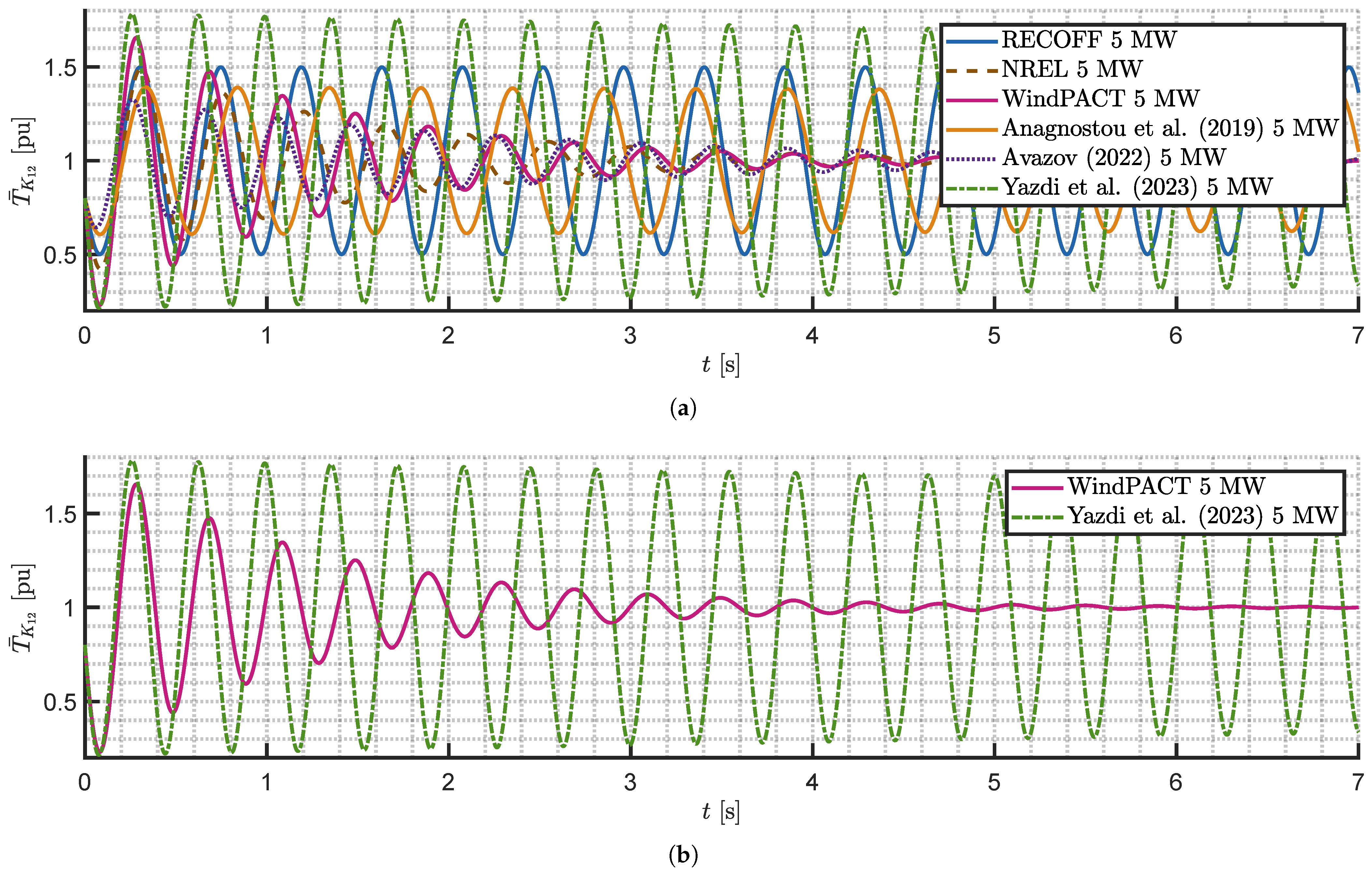
where $a_1=-0.2$, $a_2=0.01$, and ${\overline{T}}_{\mathrm{W}}={\overline{T}}_{\mathrm{e}}=1\mathrm{pu}$. The results of the numerical simulation are shown in Figure 11, which depicts the time responses of the two-mass drive train to a disturbance from equilibrium. Figure 11a illustrates the six transient responses corresponding to the six sets of per-unit parameters that have been studied in this subsection. To emphasize the quantitative and qualitative differences caused by parametric inconsistencies, two time-domain responses have been redrawn in Figure 11b, where the discrepancies are clearly evident.

Let us consider the per-unit mathematical model given in Equation (62) and compute the associated poles for the six sets of per-unit parameters analyzed in this subsection. The resulting complex conjugate poles, $s_{1,2}=\sigma \pm i{\omega }_d$, are listed in

Table 18. Drive train torsional vibration analysis.

Drive Train	Pole	Natural Angular	Damping	Damped
	Pair	Velocity [$\mathrm{rad}/\mathrm{s}$]	Ratio	Frequency [$\mathrm{Hz}$]
RECOFF $5\mathrm{MW}$	$0.0000\pm 14.1843i$	$14.184$	0	-
NREL $5\mathrm{MW}$	$-0.7060\pm 14.0224i$	$14.040$	$0.050286$	$2.2317$
WindPACT $5\mathrm{MW}$	$-0.7963\pm 15.6562i$	$15.676$	$0.050794$	$2.4918$
[34]	$-0.0069\pm 12.4703i$	$12.470$	$0.00055130$	$1.9847$
[35]	$-0.4420\pm 15.7272i$	$15.733$	$0.028095$	$2.5031$
[38]	$-0.0236\pm 17.2251i$	$17.225$	$0.0013707$	$2.7414$

.

On average, each transient exhibits an oscillatory response frequency of approximately $2.37\mathrm{Hz}$. The time-domain responses are strongly influenced by the damping coefficient ${\overline{D}}_{12}$. In particular, the oscillations corresponding to the parameter sets reported in [15] (NREL $5\mathrm{MW}$), [16,17] (WindPACT $5\mathrm{MW}$), and [35,36,37] decay rapidly, within approximately 6 to $11\mathrm{s}$, due to their relatively large negative $\left|\sigma \right|$ values.

In contrast, the poles associated with [34,38] (see Table 18) exhibit small negative $\left|\sigma \right|$ values, resulting in a very slow decay of the oscillations. These responses vanish after approximately $211.76\mathrm{s}$ for [38] and about $727.27\mathrm{s}$ for [34].

Finally, for [14] (RECOFF $5\mathrm{MW}$), the pole pair $s_{1,2}$ lies on the imaginary axis of the s-plane; therefore, the drive train is undamped, and the torque oscillations do not decay over time.

It is noted that the per-unit drive train characteristic equation and modal response components remain unchanged after setting $f_b\equiv {\omega }_b=2\pi 50\mathrm{rad}/\mathrm{s}$. This result is expected, as it is well known that the per-unit conversion fully preserves the qualitative behaviour of the original representation in real quantities [3,40]. Hence, the previous analysis of the per-unit two-mass drive train time-domain response remains unaltered when setting $f_b\equiv {\omega }_b=2\pi 60\mathrm{rad}/\mathrm{s}$, as is the case for the per-unit data presented in Table 10, Table 11 and Table 15.

4.3. On the Consequences of Inconsistent Formulations for the Per-Unit Two-Mass Drive Train

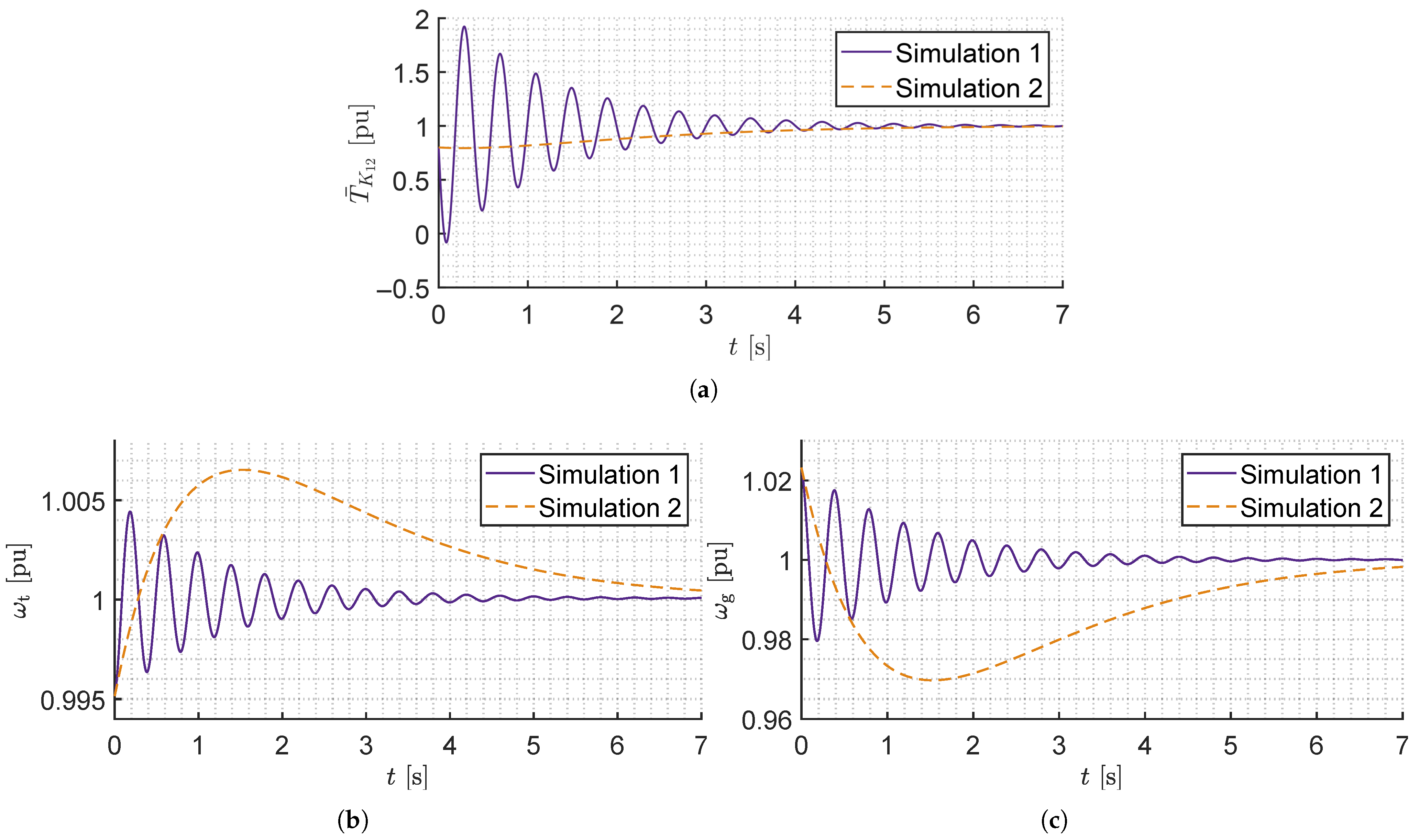
In order to highlight and illustrate the importance of using a dimensionally consistent per-unit two-mass drive train model and its corresponding per-unit parameters, a time-domain simulation was conducted using the per-unit block diagram shown in Figure 2 and that shown in Figure 10; these two representations are clearly different. It is known that the drive train torsional stiffness coefficients are related by ${\hat{K}}_{12}={\omega }_b{\overline{K}}_{12}$, as can be derived from Figure 10. In contrast, it is often considered that ${\hat{K}}_{12}:={\overline{K}}_{12}$, see [35,36,37] and Figure 2. The per-unit parameters in this time-domain simulation are those listed in Table 15 (WindPACT $5\mathrm{MW}$), and the initial conditions at $t=0\mathrm{s}$ are the same as those in Equations (63)–(65). The simulation results are shown in Figure 12.

In Figure 12, it is evident that the dynamical behaviour obtained with the dimensionally homogeneous and consistent formulation (Simulation 1) differs markedly from that of the dimensionally inconsistent formulation (Simulation 2). Although the settling time appears to remain approximately constant at $6.28\mathrm{s}$, the damping ratio in Simulation 2 (approximately 0.98623) is significantly higher than that of Simulation 1 (0.050794) (see Table 18). Moreover, Simulation 2 does not exhibit the torsional oscillations associated with the damped frequency of $0.0213\mathrm{Hz}$.

Therefore, this potential source of error and misunderstanding may lead to significant deviations from the expected results in transient studies of wind energy systems.

4.4. Limitations and Future Work

The applicability of the results presented herein is limited to two-mass drive train wind turbine models and may not be directly transferable to the analysis of direct-drive wind turbine generation systems, in which shaft torsional oscillations are typically neglected, such as the Type IV Wind Energy Conversion Systems (WECSs) [41,42].

The presented per-unit data may be used for WECS simulation, including Type IV WECSs [43]. Nonetheless, for wind turbines in WECSs, technologies such as digital twins may be used for monitoring, simulation, and predictive analysis [44]. Such digital twins may not strictly correspond to physical models, but also to data-driven approaches which may be combined to give rise to hybrid modeling [44,45].

Another limitation is that the included wind turbine data and parameters in [14,15,16,17] correspond to a nominal electrical angular velocity of $2\pi 60\mathrm{rad}/\mathrm{s}$. Hence, more open-access datasheets and corresponding design information files for wind turbines with a nominal electrical angular velocity of $2\pi 50\mathrm{rad}/\mathrm{s}$ are needed, which is difficult, as such information is often confidential [45].

The presented per-unit data, specifically turbine and generator inertia, may be used in future research to investigate the fault ride through capabilities of WECSs to meet grid code requirements [46,47].

Future potential research avenues include the development of a per-unit three-mass drive train model of a wind turbine for standardization purposes and the development of a planetary gearbox per-unit model to study transient vibration dynamics of the drive train model, along with the calculation of corresponding sets of unambiguous, traceable, and dimensionally homogeneous per-unit parameters to ensure benchmarking capabilities for a set of representative Reference Wind Turbines covering a wide range of nominal power levels.

5. Conclusions

This paper addressed the undesirable current scenario in the wind energy literature that lacks standardized per-unit drive train models and their corresponding per-unit parameters. The multi-domain Bond Graph formalism was employed here for obtaining consistent, fully unambiguous and dimensionally homogeneous per-unit parameters and a corresponding per-unit model for a two-mass wind turbine drive train. The applicability of the presented method was demonstrated by converting original data in real quantities for higher-order drive train systems into per-unit data for a reduced-order two-mass drive train model. Only original data of those wind turbines that may serve as representative traceable Reference Wind Turbines were carefully chosen. Furthermore, we purposefully selected a convenient variety of wind turbines to cover a practical, wide range of nominal power. The open-access characteristics of the model and the traceability of the computed per-unit data allow valuable, trustworthy, and reproducible simulation results. This is an important contribution, as the undesirable current modeling scenario makes benchmarking capabilities and comparison of results among the diverse wind-turbine-related literature difficult.

References

1. Travis, I. Per-Unit Quantities. Trans. Am. Inst. Electr. Eng. 1937, 56, 22–28. [Google Scholar] [CrossRef]
2. Knudsen, H.; Nielsen, J.N. Introduction to the Modelling of Wind Turbines. In Wind Power in Power Systems, 2nd ed.; Ackermann, T., Ed.; John Wiley & Sons: Chichester, UK, 2012; Chapter 34; pp. 769–797. [Google Scholar]
3. Rodríguez-Guillén, J.; Salas-Cabrera, R.; García-Vite, P.M. Bond Graph as a formal methodology for obtaining a wind turbine drive train model in the per-unit system. Int. J. Electr. Power Energy Syst. 2021, 124, 106382. [Google Scholar] [CrossRef]
4. Borutzky, W. Bond Graph Methodology, 1st ed.; Springer: London, UK, 2010. [Google Scholar] [CrossRef]
5. Bakka, T.; Karimi, H.R. Bond graph modeling and simulation of wind turbine systems. J. Mech. Sci. Technol. 2013, 27, 1843–1852. [Google Scholar] [CrossRef][Green Version]
6. Borutzky, W. Bond Graphs for Modelling, Control and Fault Diagnosis of Engineering Systems, 2nd ed.; Springer International Publishing: Berlin/Heidelberg, Germany, 2017. [Google Scholar] [CrossRef]
7. Chen, J.; Li, C.; Fan, J.; Gao, K.; Sun, C.; Zhang, G. Fault diagnosis of landing gear retraction system with bond graph under uncertain conditions. Rev. Sci. Instrum. 2024, 95, 075113. [Google Scholar] [CrossRef]
8. Karimi, M.; Mustapha, Z.; Khaouch, Z.; Touairi, S. Modeling and control of a novel mechatronic model of a 750 kW-FSWT with power-splitting transmission using RBF neural network: A bond graph approach. Simulation 2024, 100, 1153–1174. [Google Scholar] [CrossRef]
9. Chen, Q.; Xu, R.; Shen, J.; Xu, M.; Pan, J.; Zhang, J.; Wang, J. Bond graph modeling of electric vehicle drive system considering electromechanical coupling effect. J. Braz. Soc. Mech. Sci. Eng. 2025, 47, 232. [Google Scholar] [CrossRef]
10. Gawthrop, P.J.; Pan, M.; Rajagopal, V. Energy-based modelling of single actin filament polymerization using bond graphs. J. R. Soc. Interface 2025, 22, 20240404. [Google Scholar] [CrossRef]
11. Taleb, M.A.; Husi, G. Dynamic Modeling of a Three-Phase BLDC Motor Using Bond Graph Methodology. Actuators 2025, 14, 523. [Google Scholar] [CrossRef]
12. Fujita, T. Modeling Hierarchical Systems in Graph Signal Processing, Electric Circuits, and Bond Graphs via Hypergraphs and Superhypergraphs. J. Eng. Res. Rep. 2025, 27, 542–592. [Google Scholar] [CrossRef]
13. Bortolotti, P.; Tarres, H.C.; Dykes, K.L.; Merz, K.; Sethuraman, L.; Verelst, D.; Zahle, F. IEA Wind TCP Task 37: Systems Engineering in Wind Energy—WP2.1 Reference Wind Turbines; Technical Report NREL/TP-5000-73492; National Renewable Energy Laboratory (NREL): Golden, CO, USA, 2019. [CrossRef]
14. Krogh, T. HAWC Load Simulation of Generic 5 MW Offshore Wind Turbine Model; Technical Report 1475(EN); Risø National Laboratory: Roskilde, Denmark, 2004.
15. Jonkman, J.; Butterfield, S.; Musial, W.; Scott, G. Definition of a 5-MW Reference Wind Turbine for Offshore System Development; Technical Report NREL/TP-500-38060; National Renewable Energy Laboratory (NREL): Golden, CO, USA, 2009. [CrossRef]
16. Dykes, K.L.; Rinker, J. WindPACT Reference Wind Turbines; Technical Report NREL/TP-5000-67667; National Renewable Energy Laboratory: Golden, CO, USA, 2018. [CrossRef]
17. Rinker, J. Microsoft Excel Files for the WindPACT Reference Models; National Laboratory of the Rockies: Golden, CO, USA, 2016.
18. Abdulabbas, A.K.; Salih, S.M.; Alawan, M.A. The Analysis of Sub-Synchronous Resonance in a Wind Farm for a Doubly-Fed Induction Generator Using Modern Analytical Method. Iraqi J. Electr. Electron. Eng. 2024, 20, 257–270. [Google Scholar] [CrossRef]
19. Verma, N.; Kumar, N.; Kumar, R. Battery energy storage-based system damping controller for alleviating sub-synchronous oscillations in a DFIG-based wind power plant. Prot. Control Mod. Power Syst. 2023, 8, 1–18. [Google Scholar] [CrossRef]
20. Sudharsan, G.S.; Karthikeyan, N.; Xavier, S.A.E.; Eswaran, T.; Rahual, S. Optimal drive train management of wind turbine using LiDAR-assisted predictive control strategy. Environ. Dev. Sustain. 2023, 27, 24195–24224. [Google Scholar] [CrossRef]
21. Shabani, H.R.; Hajizadeh, A.; Kalantar, M.; Lashgari, M.; Nozarian, M. Transient stability analysis of DFIG-based wind farm-integrated power system considering gearbox ratio and reactive power control. Electr. Eng. 2023, 105, 3719–3735. [Google Scholar] [CrossRef]
22. Eisa, S.A. Modeling dynamics and control of type-3 DFIG wind turbines: Stability, Q Droop function, control limits and extreme scenarios simulation. Electr. Power Syst. Res. 2019, 166, 29–42. [Google Scholar] [CrossRef]
23. Prajapat, G.P.; Senroy, N.; Narayan Kar, I. Stability enhancement of DFIG-based wind turbine system through linear quadratic regulator. IET Gener. Transm. Distrib. 2018, 12, 1331–1338. [Google Scholar] [CrossRef]
24. Amutha, N.; Kumar, B.K. Effect of Modeling of Induction Generator Based Wind Generating Systems on Determining CCT. IEEE Trans. Power Syst. 2013, 28, 4456–4464. [Google Scholar] [CrossRef]
25. Gonzalez-Rodriguez, A.G.; Roldan-Fernandez, J.M.; Nieto-Nieto, L.M. Unveiling Inertia Constants by Exploring Mass Distribution in Wind Turbine Blades and Review of the Drive Train Parameters. Machines 2023, 11, 908. [Google Scholar] [CrossRef]
26. Zhao, H.; Wu, Q.; Sørensen, P.; Bech, J.; Andresen, B. Implementation of draft IEC Generic Model of Type 1 Wind Turbine Generator in PowerFactory and Simulink. In 12th Wind Integration Workshop in London 2013; Energynautics GmbH: Darmstadt, Germany, 2013; pp. 377–384. [Google Scholar]
27. IEC. Wind Energy Generation Systems—Part 27-1: Electrical Simulation Models for Wind Power Generation—Wind Turbines; Technical Report IEC 61400-27-1; International Electrotechnical Commission: Geneva, Switzerland, 2020. [Google Scholar]
28. Clark, K.; Miller, N.W.; Sanchez-Gasca, J.J. Modeling of GE Wind Turbine-Generators for Grid Studies; Technical Report; One River Road: Schenectady, NY, USA, 2010. [Google Scholar]
29. Zhang, X.; He, W.; Hu, J. Impact of Inertia Control of DFIG-based WT on Torsional Vibration in Drivetrain. IEEE Trans. Sustain. Energy 2020, 11, 2525–2534. [Google Scholar] [CrossRef]
30. Muyeen, S.M.; Tamura, J.; Murata, T. Stability Augmentation of a Grid-Connected Wind Farm, 1st ed.; Springer: London, UK, 2009. [Google Scholar] [CrossRef]
31. Akhmatov, V. Analysis of Dynamic Behaviour of Electric Power Systems with Large Amount of Wind Power; Technical University of Denmark: Kongens Lyngby, Denmark, 2003. [Google Scholar]
32. Rahimi, M.; Asadi, M. Control and dynamic response analysis of full converter wind turbines with squirrel cage induction generators considering pitch control and drive train dynamics. Int. J. Electr. Power Energy Syst. 2019, 108, 280–292. [Google Scholar] [CrossRef]
33. Govindan, S.S. 4 - IoT-based smart monitoring panel for floating horizontal axis wind turbine. In Recent Advancement of IoT Devices in Pollution Control and Health Applications; Roy, S., Tran, T.A., Natarajan, K., Eds.; Advances in Pollution Research; Woodhead Publishing: Sawston, UK, 2023; pp. 37–51. [Google Scholar] [CrossRef]
34. Anagnostou, G.; Kunjumuhammed, L.P.; Pal, B.C. Dynamic State Estimation for Wind Turbine Models With Unknown Wind Velocity. IEEE Trans. Power Syst. 2019, 34, 3879–3890. [Google Scholar] [CrossRef]
35. Avazov, A. AC Connection of Wind Farms to Transmission System: From Grid-Following to Grid-Forming. Ph.D. Theses, Katholieke Universiteit te Leuven, Leuven, Belgium, 2022. [Google Scholar]
36. Liu, S.; Wu, H.; Bosma, T.; Wang, X. Impact of DC-Link Voltage Control on Torsional Vibrations in Grid-Forming PMSG Wind Turbines. IEEE Trans. Energy Convers. 2024, 39, 2631–2642. [Google Scholar] [CrossRef]
37. Wagh, C.; Boukhenfouf, J.; Colas, F.; Rouco, L.; Guillaud, X. Non-linear interaction between a synchronous generator and grid-forming-controlled wind turbines – inertial effect enhancement and oscillation mitigation. Wind Energy Sci. 2025, 10, 2597–2614. [Google Scholar] [CrossRef]
38. Yazdi, S.S.H.; Shokri-Kalandaragh, Y.; Bagheri, M. Power system stability improvement considering drive train oscillations of virtual synchronous generator-regulated type-4 wind turbines. IET Renew. Power Gener. 2023, 17, 579–603. [Google Scholar] [CrossRef]
39. Prajapat, G.P.; Bhui, P.; Senroy, N.; Kar, I.N. Modelling and estimation of gear train backlash present in wind turbine driven DFIG system. IET Gener. Transm. Distrib. 2018, 12, 3527–3535. [Google Scholar] [CrossRef]
40. Venkatramanan, D.; Dhople, S. Per-Unit Modeling via Similarity Transformation. IEEE Trans. Energy Convers. 2023, 38, 825–837. [Google Scholar] [CrossRef]
41. O’Malley, M.; Holttinen, H.; Cutululis, N.; Vrana, T.K.; King, J.; Gevorgian, V.; Wang, X.; Rajaei-Najafabadi, F.; Hadjileonidas, A. Grand challenges of wind energy science—Meeting the needs and services of the power system. Wind Energy Sci. 2024, 9, 2087–2112. [Google Scholar] [CrossRef]
42. Kassoumi, A.E.; Lamhamdi, M.; Mouhsen, A.; Fdaili, M.; Aboudrar, I.; Mouhsen, A. Nonlinear backstepping and model predictive control for grid-connected permanent magnet synchronous generator wind turbines. Int. J. Electr. Comput. Eng. 2025, 15, 5091–5105. [Google Scholar] [CrossRef]
43. Ma, Y.; Xu, J.; Li, G.; Wang, K. Torsional Oscillation Damping Analysis and Suppression Strategy for PMSG-based Wind Generation System. J. Mod. Power Syst. Clean Energy 2024, 13, 439–451. [Google Scholar] [CrossRef]
44. Kandemir, E.; Hasan, A.; Kvamsdal, T.; Abdel-Afou Alaliyat, S. Predictive digital twin for wind energy systems: A literature review. Energy Inform. 2024, 7, 68. [Google Scholar] [CrossRef]
45. Jiménez-Ruiz, J.; Honrubia-Escribano, A.; Gómez-Lázaro, E. Enhancing Wind Turbine Dynamic Transient Simulation Using Deep Learning. In Proceedings of the 2025 IEEE 19th International Conference on Compatibility, Power Electronics and Power Engineering (CPE-POWERENG), Antalya, Turkey, 20–22 May 2025; pp. 1–6. [Google Scholar] [CrossRef]
46. Zenhom, I.A.; Marei, M.I.; Mohamed, A.M.I. Modelling, analysis, and stability assessment of wind turbine generator connected to a low inertia AC-DC microgrid with frequency support capability. Sci. Rep. 2025, 15, 44412. [Google Scholar] [CrossRef]
47. Verma, P.; K., S.; Dwivedi, B. Comprehensive investigation on doubly fed induction generator-Wind farms at fault ride through capabilities: Technical difficulties and improvisations. Energy Sources Part A 2025, 47, 3621–3653. [Google Scholar] [CrossRef]
Figure 1. Block diagram for a two-mass drive train as appears in [26].
Mca 31 00051 g001
Figure 2. Block diagram for a two-mass drive train as appears in [27].
Mca 31 00051 g002
Figure 3. Block diagram for a two-mass drive train as appears in [28].
Mca 31 00051 g003
Figure 4. Block diagram for a two-mass drive train as appears in [29].
Mca 31 00051 g004
Figure 5. The BG power-conserving TF element is depicted.
Mca 31 00051 g005
Figure 6. Iconic diagram for the two-mass wind turbine drive train model.
Mca 31 00051 g006
Figure 7. Bond Graph corresponding with the iconic diagram of the wind turbine two-mass drive train model shown in Figure 6.
Mca 31 00051 g007
Figure 8. Propagation of the base quantities throughout the two-mass drive train Bond Graph model.
Mca 31 00051 g008
Figure 9. Per-unit system Bond Graph corresponding to the application of the Bond Graph methodology to the Bond Graph shown in Figure 7.
Mca 31 00051 g009
Figure 10. Block diagram corresponding to the two-mass drive train Bond Graph model in the pu system shown in Figure 9 (cf. [27,28]).
Mca 31 00051 g010
Figure 11. Time-domain response of the torsionally elastic shaft torque component, T ¯ K 12 [ pu ] , in a two-mass drive train following a disturbance from equilibrium: (a) six simulation transient responses corresponding to the six sets of per-unit parameters that have been studied in this subsection [14,15,16,17,34,35,36,37,38]. (b) Two simulation transient responses considering the parameter data reported in [16,17] (WindPACT 5 MW ) and [38].
Mca 31 00051 g011
Figure 12. Two-mass drive train time-domain response to a disturbance from equilibrium of a consistent formulation where K ^ 12 = ω b K ¯ 12 (Simulation 1) and an inconsistent formulation where K ^ 12 = K ¯ 12 (Simulation 2): (a) Torsionally elastic torque component of the shaft in pu . (b) Rotor axis angular speed of the wind turbine in pu . (c) Generator axis angular speed in pu .
Mca 31 00051 g012