Lie Point and Q-Conditional Symmetries, Exact Solutions, and Conservation Laws for a Reaction–Diffusion System in Mathematical Biology

Abstract

This study investigates the Lie point and Q-conditional symmetries of a classical two-component reaction–diffusion system in one spatial dimension. The symmetry classifications for the reaction–diffusion system and corresponding symmetry reductions are provided. Employing Ibragimov’s method, we construct conservation laws for the governing system, offering insights into its invariant properties. Additionally, by applying symmetry reduction techniques, new exact solutions are obtained. These solutions demonstrate the practical utility of our approach and enhance our understanding of the system’s behavior and characteristics.

1. Introduction

The reaction–diffusion (RD) system is defined as

$${\partial }_t{u}^i=F^i(u^i,{\theta }_i)\Delta u^i+R^i(u^1,u^2,\dots ,u^m),i=1,2,\dots ,m,$$

(1)

where $u^i=u^i(x,t)$, $i=1,2,\dots ,m$ denote the dependent variables (e.g., densities of species or components), $\Delta$ is the Laplace operator, and system (1) serves as a fundamental mathematical model for diffusion–reaction processes in various scientific fields, such as physics, biology, finance, and ecology [1,2,3,4,5,6,7]. This system combines both diffusion and reaction dynamics. In population dynamics, for example, it models the spatiotemporal evolution of population densities, where the diffusion term represents the random movement or migration of individuals, and the reaction term accounts for population interactions such as reproduction, competition, and predation. By adjusting the parameters of the reaction terms, the model can be applied to a variety of phenomena, including material diffusion, population dynamics, and market fluctuations, making it a versatile and powerful tool for both theoretical and applied research.

A specific example of a reaction–diffusion system is given by the model

$$\begin{array}{cc}\hfill & u_t=d_1{u}_{xx}-a{u}^2+2bv+cu-k{u}^2-2kuv,\hfill \\ \hfill & v_t=d_2{v}_{xx}+{\displaystyle \frac{a}{2}}{u}^2-bv,\hfill \end{array}$$

(2)

where u and v are the dependent variables representing the densities of isolated and paired Myxobacteria, respectively, at a given location. This model is significant for simulating the effect of social behavior on the movement of Myxobacteria [8]. It describes the spatial dynamics of these bacteria as they move along a straight line. In 2024, Estavoyer and Lepoutre studied the traveling wave solutions of this model [9]. The above reaction–diffusion system can be viewed as a generalization of the classical Fisher-KPP equation [10], which is recovered by setting $a=b=0$ and $v=0$ at $t=0$.

Coupled reaction–diffusion systems present analytical challenges. In particular, nonlinear coupling often prevents a systematic framework for symmetry classification and reduction, resulting in a limited number of exact solutions. This limitation affects the verification of numerical methods and the analysis of solution stability. The isolated-paired Myxobacteria model proposed by Calvez et al. provides a specific example of these challenges. Although it describes key aspects of bacterial collective motion, most studies have relied on numerical simulations. As a result, the analytical structure of the system and the effects of different parameter regimes are not fully characterized.

Lie point symmetry is a classical technique for analyzing nonlinear partial differential equations (PDEs). In the 1870s, the Norwegian mathematician Sophus Lie introduced the theory of Lie groups, now referred to as Lie symmetry theory [11]. Lie symmetry methods allow the construction of exact solutions and have applications such as the classification of equations with arbitrary parameters [12], linearization, and the derivation of conservation laws [13]. By systematically exploiting symmetries, this approach can reduce complex PDEs to simpler forms, facilitating the analysis of their structure.

For certain reaction–diffusion systems that are difficult to treat using the classical Lie symmetry method—typically those with strong nonlinear coupling or multi-component interactions—the Q-conditional (nonclassical) symmetry approach can be applied. In 1969, Bluman and Cole extended the classical Lie symmetry theory and proposed the nonclassical method [14]. Fushchich and collaborators developed the theory of Q-conditional symmetry. By imposing an invariant surface condition, Q-conditional symmetry can identify additional symmetry generators, which may be useful for analyzing more complex nonlinear models. A limitation of this method is that the determining equations are highly nonlinear, and no general algorithmic solution procedure exists. Further extensions of the nonclassical (or conditional) symmetry method include the concepts of weak symmetries and side conditions (differential constraints), introduced by Olver and Rosenau [15,16]. A comprehensive exposition of nonclassical and conditional symmetries can be found in the CRC Handbook chapter by Olver and Vorob’ev [17]. Canonical examples, along with broader overviews of symmetry reduction via nonclassical or conditional symmetries, are presented by Clarkson and Winternitz [18,19]. As research on conditional symmetries progresses, there has been an increasing focus on their practical applications. The conditional symmetry approach is now widely used to address a variety of real-world problems in contemporary studies [20,21,22].

In this study, we investigate the Myxobacteria reaction–diffusion system. A symmetry classification and reduction are performed, followed by the construction of exact analytical solutions. These solutions serve as benchmarks for numerical validation and provide insights into the influence of model parameters on the system’s behavior.

The organization of this paper is as follows: In Section 2, we classify the Lie point and Q-conditional symmetries and present symmetry reductions for system (2). In Section 3, we construct the exact solutions for system (2). In Section 4, we apply Ibragimov’s new conservation theorem to derive the conservation laws for system (2). Section 5 concludes the paper.

2. Lie Point and $\mathit{Q}$-Conditional Symmetries of the System (2)

2.1. Lie Point Symmetry Analysis and Reductions

We consider the invariance of a one-parameter Lie transformation group in $(x,t,u,v)$:

$$\begin{array}{cc}\hfill & x\to x+\epsilon \xi (x,t,u,v),\hfill \\ \hfill & t\to t+\epsilon \tau (x,t,u,v),\hfill \\ \hfill & u\to u+\epsilon \eta (x,t,u,v),\hfill \\ \hfill & v\to v+\epsilon \psi (x,t,u,v),\hfill \end{array}$$

(3)

where $\epsilon$ is a group parameter, and $\xi ,\tau ,\eta ,\psi$ are infinitesimals. The system (2) is invariant under the Lie point transformation group, with a symmetry operator of the form:

$$\begin{array}{c}\hfill X=\xi (x,t,u,v){\displaystyle \frac{\partial }{\partial x}}+\tau (x,t,u,v){\displaystyle \frac{\partial }{\partial t}}+\eta (x,t,u,v){\displaystyle \frac{\partial }{\partial u}}+\psi (x,t,u,v){\displaystyle \frac{\partial }{\partial v}},\end{array}$$

(4)

where $\xi (x,t,u,v),\tau (x,t,u,v),\eta (x,t,u,v),\psi (x,t,u,v)$ are undetermined functions. The invariance of partial differential Equations (2) is given by Lie’s invariance condition

$$\begin{array}{cc}\hfill & {Pr}^{(2)}X({\Delta }_1){|}_{{\Delta }_1=0,{\Delta }_2=0}=0,\hfill \\ \hfill & {Pr}^{(2)}X({\Delta }_2){|}_{{\Delta }_1=0,{\Delta }_2=0}=0,\hfill \end{array}$$

(5)

where ${Pr}^{(2)}X$ is the second prolongation of the vector field X, and

$$\begin{array}{cc}\hfill & {\Delta }_1=d_1{u}_{xx}-a{u}^2+2bv+cu-k{u}^2-2kuv-u_t,\hfill \\ \hfill & {\Delta }_2=d_2{v}_{xx}+{\displaystyle \frac{a}{2}}{u}^2-bv-v_t.\hfill \end{array}$$

(6)

From (5), we obtain the following determining equations

$$\begin{array}{cc}\hfill & {\tau }_x=0,{\tau }_u=0,{\tau }_v=0,\hfill \\ \hfill & {\xi }_u=0,{\xi }_v=0,\hfill \\ \hfill & {\eta }_{uu}=0,{\eta }_{uv}=0,{\eta }_{vv}=0,{\eta }_{xv}=0,\hfill \\ \hfill & {\psi }_{uu}=0,{\psi }_{uv}=0,{\psi }_{vv}=0,{\psi }_{xu}=0,\hfill \\ \hfill & v{\tau }_t-2{\xi }_x=0,(d_1-d_2){\eta }_v=0,\hfill \\ \hfill & (d_1-d_2){\psi }_u=0,\hfill \\ \hfill & 2d_1{\eta }_{xu}+{\xi }_t-d_1{\xi }_{xx}=0,\hfill \\ \hfill & 2d_2{\psi }_{xv}+{\xi }_t-d_2{\xi }_{xx}=0,\hfill \\ \hfill & (2c-4au-4ku-4kv)\eta +(2bv-a{u}^2){\eta }_v+(2a{u}^2-2cu+2k{u}^2-4bv+4kuv){\eta }_u-\hfill \\ \hfill & 2{\eta }_t+2d_1{\eta }_{xx}+(2cu-2a{u}^2-2k{u}^2+4bv-4kuv){\tau }_t+(4b-4ku)\psi =0,\hfill \\ \hfill & 2au\eta +(a{u}^2-2bv){\tau }_t+(2a{u}^2-2cu+2k{u}^2-4bv+4kuv){\psi }_u\hfill \\ \hfill & -2b\psi +(2bv-a{u}^2){\psi }_v+2{\psi }_t+2d_2{\psi }_{xx}=0.\hfill \end{array}$$

(7)

The system (7) contains arbitrary parameters $a,b,c,d_1,d_2,k$. For arbitrary parameters $a,b,c,d_1,d_2$ and k, solving this system yields the following two independent operators, which form a trivial Lie algebra:

$$X_1={\displaystyle \frac{\partial }{\partial x}},X_2={\displaystyle \frac{\partial }{\partial t}}.$$

(8)

Additionally, in other special cases for parameters $a,b,c,d_1,d_2,k$, the system (2) allows the nontrivial Lie algebra. The symmetry classification of system (2) is presented in

Table 1. Lie symmetry operators of system (2).

Ordinal Number	Reaction Terms	Restrictions	Nontrivial Symmetry Operators
1	$2bv+cu$ $-bv$	$a=k=0$, b≠0	$X_3=u{\displaystyle \frac{\partial }{\partial u}}+v{\displaystyle \frac{\partial }{\partial v}}$
2	$2bv-bu$ $-bv$	$a=k=0$, $c=-b$ ≠ 0	$X_3=u{\displaystyle \frac{\partial }{\partial u}}+v{\displaystyle \frac{\partial }{\partial v}},$ $X_4=x{\displaystyle \frac{\partial }{\partial x}}+2t{\displaystyle \frac{\partial }{\partial t}}-2btu{\displaystyle \frac{\partial }{\partial u}}+(2bt+2)v{\displaystyle \frac{\partial }{\partial v}}$
3	$2bv+cu$ $-bv$	$a=k=0$, $d_1=d_2=d$	$X_3=e^{(b+c)t}v{\displaystyle \frac{\partial }{\partial u}},X_4=(u+{\displaystyle \frac{2bv}{b+c}}){\displaystyle \frac{\partial }{\partial u}},$ $X_5=-{\displaystyle \frac{2bv}{b+c}}{\displaystyle \frac{\partial }{\partial u}}+v{\displaystyle \frac{\partial }{\partial v}},X_6=t{\displaystyle \frac{\partial }{\partial x}}-{\displaystyle \frac{x}{2d}}(u{\displaystyle \frac{\partial }{\partial u}}+v{\displaystyle \frac{\partial }{\partial v}}),$ $X_7=e^{-(b+c)t}\left[(-{\displaystyle \frac{2bu}{b+c}}-{\displaystyle \frac{4b^{2}v}{{(b+c)}^2}}){\displaystyle \frac{\partial }{\partial u}}+(u+{\displaystyle \frac{2bv}{b+c}}){\displaystyle \frac{\partial }{\partial v}}\right],$ $X_8=x{\displaystyle \frac{\partial }{\partial x}}+2t{\displaystyle \frac{\partial }{\partial t}}+(2ctu+4btv){\displaystyle \frac{\partial }{\partial u}}-2btv{\displaystyle \frac{\partial }{\partial v}},$ $X_9=xt{\displaystyle \frac{\partial }{\partial x}}+t^2{\displaystyle \frac{\partial }{\partial t}}+\left[(c{t}^2-{\displaystyle \frac{t}{2}}-{\displaystyle \frac{x^2}{4d}})u+2b{t}^{2}v\right]{\displaystyle \frac{\partial }{\partial u}}-$ $(b{t}^2+{\displaystyle \frac{t}{2}}+{\displaystyle \frac{x^2}{4d}})v{\displaystyle \frac{\partial }{\partial v}}$
4	$cu-k{u}^2-2kuv$ 0	$a=b=0$	$X_3=-{\displaystyle \frac{x}{2}}{\displaystyle \frac{\partial }{\partial x}}-t{\displaystyle \frac{\partial }{\partial t}}+u{\displaystyle \frac{\partial }{\partial u}}+(v-{\displaystyle \frac{c}{2k}}){\displaystyle \frac{\partial }{\partial v}}$
5	$2auv+cu$ ${\displaystyle \frac{a}{2}}{u}^2$	$b=0,a=-k$	$X_3=-{\displaystyle \frac{x}{2}}{\displaystyle \frac{\partial }{\partial x}}-t{\displaystyle \frac{\partial }{\partial t}}+u{\displaystyle \frac{\partial }{\partial u}}+(v+{\displaystyle \frac{c}{2a}}){\displaystyle \frac{\partial }{\partial v}}$

. Details of the calculation process can be found in Appendix A.1.

Remark 1. 

Table 1 presents the Lie symmetry operators of system (2), classified according to parameter restrictions, excluding trial cases. These symmetries highlight the possible forms of the equation under varying parameters, supporting the construction of exact solutions and conservation laws.

The Lie symmetry reduces the partial differential equations to ordinary differential equations (ODEs) through the symmetry reduction technique. In

Table 2. $Ans\ddot{a}tze$ and reduced systems of ODEs for Table 1.

	Generator	$\mathbf{Ans}\ddot{\mathit{a}}\mathbf{tze}$	Systems of ODEs
1	$X_1+X_3$	$u(x,t)=e^x{\phi }_1(t)$ $v(x,t)=e^x{\phi }_2(t)$	${\phi }_1^{\prime }-2b{\phi }_2-(c+d_1){\phi }_1=0$ ${\phi }_2^{\prime }+(b-d_2){\phi }_2=0$
2	$X_4$	$u(x,t)=e^{-bt}{\phi }_1(z),z={\displaystyle \frac{x^2}{t}}$ $v(x,t)=t^{-1}{e}^{-bt}{\phi }_2(z)$	$4d_{1}z{\phi }_1^{″}+(2d_1+z){\phi }_1^{\prime }+2b{\phi }_2=0$ $4d_{2}z{\phi }_2^{″}+(2d_2+z){\phi }_2^{\prime }+{\phi }_2=0$
3	$X_8$	$u(x,t),v(x,t)$	$d{u}_{xx}+{\displaystyle \frac{x}{2t}}{u}_x=0$ $d{v}_{xx}+{\displaystyle \frac{x}{2t}}{v}_x=0$
4	$X_3$	$u(x,t)=t^{-1}{\phi }_1(z),z={\displaystyle \frac{x^2}{t}}$ $v=t^{-1}{\phi }_2(z)+{\displaystyle \frac{c}{2k}}$	$4d_1{z}^3{\phi }_1^{″}+(6d_1{z}^2-z){\phi }_1^{\prime }+{\phi }_1-k{\phi }_1^2-2k{\phi }_1{\phi }_2=0$ $4d_2{z}^3{\phi }_2^{″}+(6d_2{z}^2-z){\phi }_2^{\prime }+{\phi }_2=0$
5	$X_3$	$u(x,t)=t^{-1}{\phi }_1(z),z={\displaystyle \frac{x^2}{t}}$ $v=t^{-1}{\phi }_2(z)-{\displaystyle \frac{c}{2a}}$	$4d_{1}z{\phi }_1^{″}+(2d_1+z){\phi }_1^{\prime }+{\phi }_1+2a{\phi }_1{\phi }_2=0$ $4d_{2}z{\phi }_2^{″}+(2d_2+z){\phi }_2^{\prime }+{\displaystyle \frac{a}{2}}{\phi }_1^2+{\phi }_2=0$

, the symmetry reduction results of Table 1 under selected symmetries are given. For the detailed calculation process, please refer to Appendix A.3.

Remark 2. 

Table 2 presents the reduced systems of ordinary differential equations (ODEs) corresponding to the selected Lie symmetry generators classified in Table 1. These simplified ODEs are more easily solvable mathematically. Each generator leads to a distinct form of the reduced system.

2.2. Q-Conditional Symmetry Analysis and Reductions

The operator

$$Q=\tau (x,t,u,v){\displaystyle \frac{\partial }{\partial t}}+\xi (x,t,u,v){\displaystyle \frac{\partial }{\partial x}}+\eta (x,t,u,v){\displaystyle \frac{\partial }{\partial u}}+\psi (x,t,u,v){\displaystyle \frac{\partial }{\partial v}},{\tau }^2+{\xi }^2\ne 0$$

(9)

is the Q-conditional symmetry of the system (2) if the following invariance conditions are satisfied

$$\begin{array}{cc}\hfill & {Pr}^{(2)}Q({\Delta }_1){|}_{\mathcal{M}}=0,\hfill \\ \hfill & {Pr}^{(2)}Q({\Delta }_2){|}_{\mathcal{M}}=0,\hfill \end{array}$$

(10)

where the coefficients $\xi (x,t,u,v),\tau (x,t,u,v),\eta (x,t,u,v),\psi (x,t,u,v)$ should be found using the well-known criterion, the operator ${Pr}^{(2)}Q$ is the second prolongation of the operator Q, ${\Delta }_1$ and ${\Delta }_2$ are from (6), and the mainifold $\mathcal{M}$ is

$$\mathcal{M}=\{{\Delta }_1=0,{\Delta }_2=0,u_t+\xi u_x-\eta =0,v_t+\xi v_x-\psi =0\}.$$

(11)

Without loss of generality, we set $\tau (x,t,u,v)=1$ [23]; then, Equation (10) yield the following nonlinear determining equations:

$$\begin{array}{cc}\hfill & {\xi }_{uu}={\xi }_{uv}={\xi }_{vv}=0,\hfill \\ \hfill & {\eta }_{vv}=0,{\psi }_{uu}=0,\hfill \\ \hfill & d_1({\eta }_{uu}-2{\xi }_{xu})+2\xi {\xi }_u=0,\hfill \\ \hfill & d_2({\psi }_{vv}-2{\xi }_{xv})+2\xi {\xi }_v=0,\hfill \\ \hfill & 2d_1({\eta }_{uv}-{\xi }_{xv})+(1+{\displaystyle \frac{d_1}{d_2}})\xi {\xi }_v=0,\hfill \\ \hfill & 2d_1{\eta }_{xv}-2{\xi }_v(\eta +a{u}^2-2bv-cu+k{u}^2+2kuv)+(1-{\displaystyle \frac{d_1}{d_2}})\xi {\eta }_v=0,\hfill \\ \hfill & 2d_2({\psi }_{uv}-{\xi }_{xu})+(1+{\displaystyle \frac{d_2}{d_1}})\xi {\xi }_u=0,2d_2{\psi }_{xu}-2{\xi }_u(\psi -{\displaystyle \frac{a}{2}}{u}^2+bv)+(1-{\displaystyle \frac{d_1}{d_2}})\xi {\psi }_u=0,\hfill \\ \hfill & 2d_1{\eta }_{xu}-d_1{\xi }_{xx}+2\xi {\xi }_x-2\eta {\xi }_u-3{\xi }_u(a{u}^2-2bv-cu+k{u}^2+2kuv)-{\displaystyle \frac{d_1}{d_2}}{\xi }_v(bv-{\displaystyle \frac{a}{2}}{u}^2)+\hfill \\ \hfill & {\xi }_t+(1-{\displaystyle \frac{d_1}{d_2}})\psi {\xi }_v=0,\hfill \\ \hfill & 2d_2{\psi }_{xv}-d_2{\xi }_{xx}+2\xi {\xi }_x-2\psi {\xi }_v-{\displaystyle \frac{d_2}{d_1}}{\xi }_u(a{u}^2-2bv-cu+k{u}^2+2kuv)-3{\xi }_v(bv-{\displaystyle \frac{a}{2}}{u}^2)+\hfill \\ \hfill & {\xi }_t+(1-{\displaystyle \frac{d_2}{d_1}})\eta {\xi }_u=0,\hfill \\ \hfill & d_1{\eta }_{xx}+{\eta }_u(a{u}^2-2bv-cu+k{u}^2+2kuv)-2{\xi }_x(\eta +a{u}^2-2bv-cu+k{u}^2+2kuv)+({\displaystyle \frac{d_1}{d_2}}-1)\psi {\eta }_v+\hfill \\ \hfill & {\displaystyle \frac{d_1}{d_2}}{\eta }_v(bv-{\displaystyle \frac{a}{2}}{u}^2)-2au\eta +2b\psi +c\eta -2ku\eta -2ku\psi -2kv\eta -{\eta }_t=0,\hfill \\ \hfill & d_2{\psi }_{xx}+({\displaystyle \frac{d_2}{d_1}}-1)\eta {\psi }_u+{\displaystyle \frac{d_2}{d_1}}{\psi }_u(a{u}^2-2bv-cu+k{u}^2+2kuv)-{\psi }_v(bv-{\displaystyle \frac{a}{2}}{u}^2)-2{\xi }_x(\psi +bv-{\displaystyle \frac{a}{2}}{u}^2)+\hfill \\ \hfill & au\eta -b\psi -{\psi }_t=0.\hfill \end{array}$$

(12)

Through complex calculations, we have Q-conditional symmetry classification results of the system (2) in

Table 3. Q-conditional symmetries of system (2).

	Reaction Terms	Reastrictions	Q-Conditional Symmetry Operators
6	$cu-(a+k)u^2-2kuv$ ${\displaystyle \frac{a}{2}}{u}^2$	$k\ne 0,a\ne 0,b=0$	$Q_1=x{\displaystyle \frac{\partial }{\partial x}}+(2t+1){\displaystyle \frac{\partial }{\partial t}}-2u{\displaystyle \frac{\partial }{\partial u}}-(2v-{\displaystyle \frac{c}{k}}){\displaystyle \frac{\partial }{\partial v}},$ $Q_2=(x+1){\displaystyle \frac{\partial }{\partial x}}+2t{\displaystyle \frac{\partial }{\partial t}}-2u{\displaystyle \frac{\partial }{\partial u}}-(2v-{\displaystyle \frac{c}{k}}){\displaystyle \frac{\partial }{\partial v}}$
7	$2bv-bu$ $-bv$	$d_1=d_2=d,$ $k=a=0,b=-c$	${\displaystyle \frac{\partial }{\partial t}}+v{\displaystyle \frac{\partial }{\partial u}}$
8	$2bv+cu$ $-bv$	$k=a=0,d_2\ne d_1$	$(d_2-d_1){\displaystyle \frac{\partial }{\partial t}}+((b{d}_1+c{d}_2)u+2b{d}_{2}v){\displaystyle \frac{\partial }{\partial u}}+$ $((d_2-d_1)u+(b{d}_1+c{d}_2)v){\displaystyle \frac{\partial }{\partial v}}$
9	$-a{u}^2$ ${\displaystyle \frac{a}{2}}{u}^2$	$k=b=c=0,a\ne 0$	$Q_1=d_1{\displaystyle \frac{\partial }{\partial t}}+(d_{1}u+d_{2}v){\displaystyle \frac{\partial }{\partial v}},$ $Q_2={\displaystyle \frac{\partial }{\partial t}}+{\displaystyle \frac{\partial }{\partial v}}$
10	$-a{u}^2$ ${\displaystyle \frac{a}{2}}{u}^2$	$k=b=c=0,$ $a\ne 0,d_1=d_2$	$Q_1=x{\displaystyle \frac{\partial }{\partial x}}+(2t+1){\displaystyle \frac{\partial }{\partial t}}-2u{\displaystyle \frac{\partial }{\partial u}}-2v{\displaystyle \frac{\partial }{\partial v}},$ $Q_2=(x+1){\displaystyle \frac{\partial }{\partial x}}+2t{\displaystyle \frac{\partial }{\partial t}}-2u{\displaystyle \frac{\partial }{\partial u}}-2v{\displaystyle \frac{\partial }{\partial v}},$ $Q_3=x{\displaystyle \frac{\partial }{\partial x}}+2t{\displaystyle \frac{\partial }{\partial t}}-2u{\displaystyle \frac{\partial }{\partial u}}+(1-2v){\displaystyle \frac{\partial }{\partial v}},$ $Q_4=x{\displaystyle \frac{\partial }{\partial x}}+2t{\displaystyle \frac{\partial }{\partial t}}-2u{\displaystyle \frac{\partial }{\partial u}}+u{\displaystyle \frac{\partial }{\partial v}}$
11	$-a{u}^2+2bv$ ${\displaystyle \frac{a}{2}}{u}^2-bv$	$d_1=d_2,k=c=0,$ $a\ne 0,b\ne 0$	$Q_1=(x+1){\displaystyle \frac{\partial }{\partial x}}+2t{\displaystyle \frac{\partial }{\partial t}}-(2u+{\displaystyle \frac{b}{a}}){\displaystyle \frac{\partial }{\partial u}}-(u+4v){\displaystyle \frac{\partial }{\partial v}},$ $Q_2=x{\displaystyle \frac{\partial }{\partial x}}+(2t+1){\displaystyle \frac{\partial }{\partial t}}-(2u+{\displaystyle \frac{b}{a}}){\displaystyle \frac{\partial }{\partial u}}-(u+4v){\displaystyle \frac{\partial }{\partial v}}$

. For the detailed calculation process, please refer to Appendix A.2.

Remark 3. 

Table 3 presents the Q-conditional symmetry classification of system (2) under the assumption $\tau (x,t,u,v)=1$. The listed symmetry operators correspond to specific parameter restrictions, revealing the system’s structure under these conditions.

It is well known that the Q-conditional symmetry can be used to reduce given two-dimensional PDEs to ODEs. In

Table 4. $Ans\ddot{a}tze$ and reduced systems of ODEs for Table 3.

	Generator	$\mathbf{Ans}\ddot{\mathit{a}}\mathbf{tze}$	Systems of ODEs
6	$Q_1$	$u=x^{-2}{\varphi }_1(\theta )$, $\theta =x{(2t+1)}^{-{\displaystyle \frac{1}{2}}}$ $v=x^{-2}{\varphi }_2(\theta )+{\displaystyle \frac{c}{2k}}$	$d_1{\theta }^2{\varphi }_1^{″}+({\theta }^3-4d_1\theta ){\varphi }_1^{\prime }+6d_1{\varphi }_1-(a+k){\varphi }_1^2-2k{\varphi }_1{\varphi }_2=0$ $d_2{\theta }^2{\varphi }_2^{″}+({\theta }^3-4d_2\theta ){\varphi }_2^{\prime }+6d_2{\varphi }_2+{\displaystyle \frac{a}{2}}{\varphi }_2^2=0$
7	Q	$u(x,t)={\varphi }_1(x)t+{\varphi }_2(x)$ $v(x,t)={\varphi }_2(x)$	$d{\varphi }_1^{″}+(2b-1){\varphi }_2-b{\varphi }_1=0$ $d{\varphi }_2^{″}-b{\varphi }_2=0$
8	Q	$u(x,t),v(x,t)$	$(d_2-d_1)u_{xx}-2bv-(b+c)u=0$ $(d_2-d_1)v_{xx}-\left(1-{\displaystyle \frac{d_1}{d_2}}\right)u-(b+c)v=0$
9	$Q_1$	$u(x,t)={\varphi }_1(x)$ $v(x,t)=-{\displaystyle \frac{d_1}{2d_2}}{\varphi }_1(x)+e^{{\displaystyle \frac{2d_2}{d_1}}t}{\varphi }_2(x)$	$d_1{\varphi }_1^{″}-a{\varphi }_1^2=0$ $d_1{\varphi }_2^{″}-2{\varphi }_2=0$
10	$Q_3$	$u(x,t)=t^{-1}{\varphi }_1(\theta )$, $\theta =x^2{t}^{-1}$ $v(x,t)={\displaystyle \frac{1}{2}}-{\displaystyle \frac{1}{2t}}{\varphi }_2(\theta )$	$4d\theta {\varphi }_1^{″}+(2d+\theta ){\varphi }_1^{\prime }-a{\varphi }_1^2+{\varphi }_1=0$ $4d\theta {\varphi }_2^{″}+(2d+\theta ){\varphi }_2^{\prime }-a{\varphi }_1^2+{\varphi }_2=0$
11	$Q_2$	$u(x,t),v(x,t)$	$d{u}_{xx}-a{u}^2+2bv+{\displaystyle \frac{1}{2t+1}}\left(2xu+{\displaystyle \frac{b}{a}}x+x{u}_x\right)=0$ $d{v}_{xx}+{\displaystyle \frac{a}{2}}{u}^2-bv+{\displaystyle \frac{1}{2t+1}}\left(xu+4xv+x{v}_x\right)=0$

, some Q-conditional symmetry reductions of system (2) are shown. For the detailed calculation process, please refer to Appendix A.4.

Remark 4. 

Table 4 shows the Q-conditional symmetry reductions of system (2), derived under specific parameter conditions. These reductions transform the PDE system into simpler ODEs, facilitating more efficient solutions.

By applying Lie point and Q-conditional (nonclassical) symmetry analyses to system (2), we performed a systematic symmetry classification and derived the corresponding reductions. The classification identifies the admitted symmetry groups for different parameter regimes, and the reductions map the original coupled PDE system to lower-dimensional ODE systems. These reduced ODEs represent distinct dynamical regimes of the model and provide a concrete framework for constructing exact solutions. In the next section, we solve representative reduced ODEs to obtain explicit solutions and examine the influence of parameter variations on the spatiotemporal evolution of the densities u and v.

3. Exact Solutions

To obtain the exact solutions for the corresponding case of the reaction–diffusion system, we need to solve the reduced system of ordinary differential equations first. Here are some new exact solutions of the system (2).

(1) After calculation, the solutions of Case 1 in Table 2 are

$$\begin{array}{cc}\hfill & {\phi }_1(t)=f_1{e}^{(c+d_1)t}-f_2{\displaystyle \frac{2b{e}^{(d_2-b)t}}{b+c+d_1-d_2}},\hfill \\ \hfill & {\phi }_2(t)=f_2{e}^{(d_2-b)t}.\hfill \end{array}$$

(13)

So we have the exact solutions for Case 1 in Table 1

$$\begin{array}{cc}\hfill & u=f_1{e}^{(c+d_1)t+x}-f_2{\displaystyle \frac{2b{e}^{(d_2-b)t+x}}{b+c+d_1-d_2}},\hfill \\ \hfill & v=f_2{e}^{(d_2-b)t+x},\hfill \end{array}$$

(14)

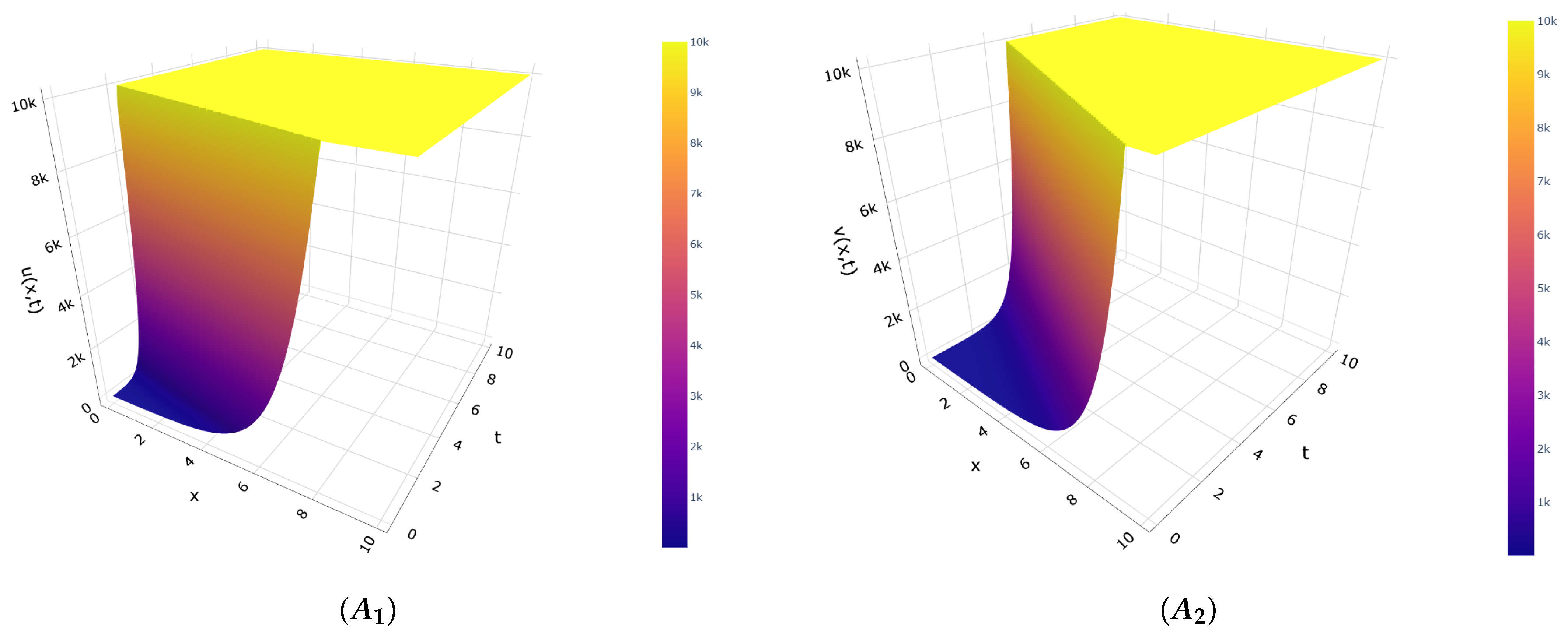
where $f_i(i=1,2)$ are arbitrary constants. The graphs of the solution in (14) for the parameters $f_1=3,f_2=1,d_1=d_2=1,b=-1$ and $c=3$ are shown in Figure 1.

(2) Similarly, after solving the ordinary differential equations of Case 7 in Table 4, we get

$$\begin{array}{cc}\hfill & {\varphi }_1(x)={\displaystyle \frac{(1-2b)(-e^{-\frac{\sqrt{b}}{\sqrt{d}}x}+e^{\frac{\sqrt{b}}{\sqrt{d}}x})x}{2\sqrt{b}\sqrt{d}}},\hfill \\ \hfill & {\varphi }_2(x)=e^{-{\displaystyle \frac{\sqrt{b}}{\sqrt{d}}}x}+e^{{\displaystyle \frac{\sqrt{b}}{\sqrt{d}}}x}.\hfill \end{array}$$

(15)

Thus, the exact solutions of Case 7 in Table 3 are given by

$$\begin{array}{cc}\hfill & u(x,t)={\displaystyle \frac{(1-2b)(-e^{-\frac{\sqrt{b}}{\sqrt{d}}x}+e^{\frac{\sqrt{b}}{\sqrt{d}}x})xt}{2\sqrt{b}\sqrt{d}}}+e^{-{\displaystyle \frac{\sqrt{b}}{\sqrt{d}}}x}+e^{{\displaystyle \frac{\sqrt{b}}{\sqrt{d}}}x},\hfill \\ \hfill & v(x,t)=e^{-{\displaystyle \frac{\sqrt{b}}{\sqrt{d}}}x}+e^{{\displaystyle \frac{\sqrt{b}}{\sqrt{d}}}x}.\hfill \end{array}$$

(16)

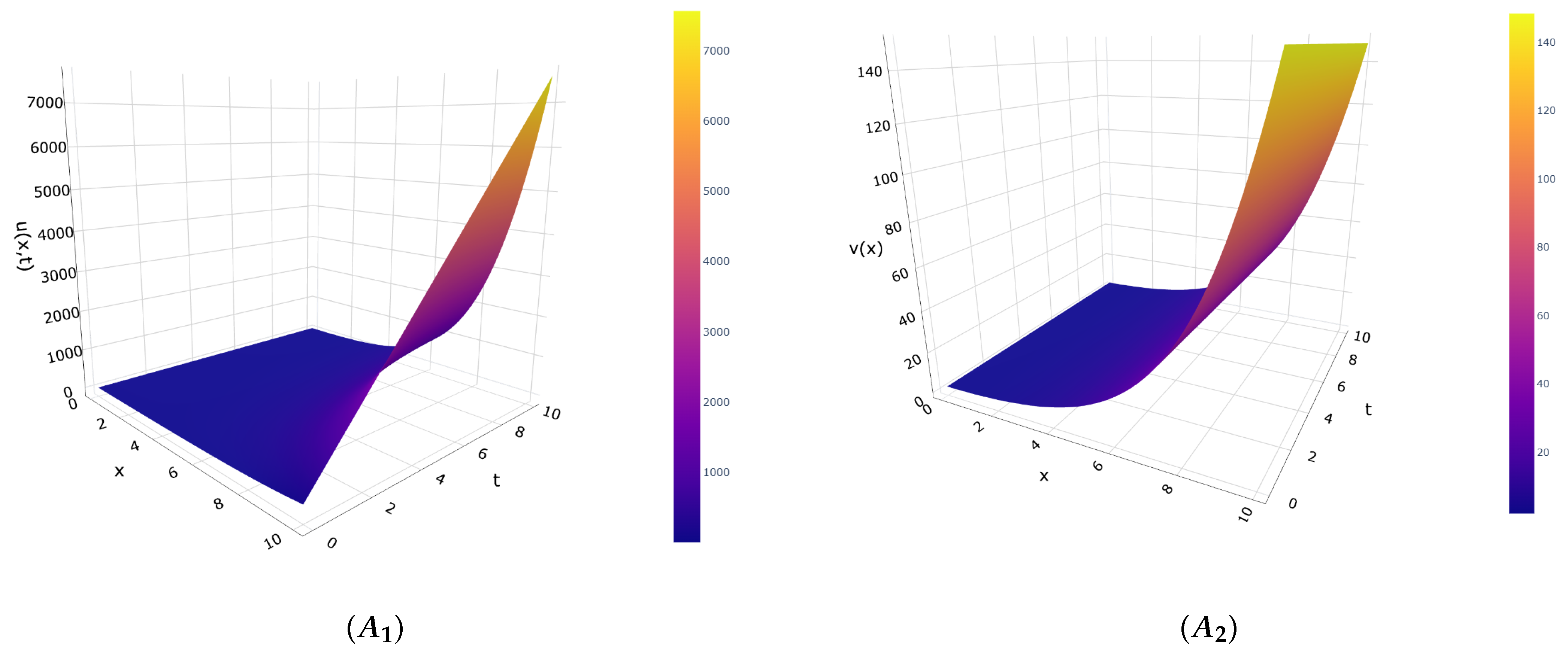
When parameter $d_1=d_2$, this simulates that the two species have the same diffusion ability, corresponding to the observed competitive symmetry in ecology. The graphs of the solution in (16) where $d_1=d_2=d=1,b={\displaystyle \frac{1}{4}}$ are given in Figure 2.

(3) The solutions of a reduced system for Case 9 in Table 4 are

$$\begin{array}{cc}\hfill & {\varphi }_1(x)={\displaystyle \frac{6^{1/3}}{{\left(\frac{a}{d_1}\right)}^{1/3}}}\wp \left({\displaystyle \frac{{\left(\frac{a}{d_1}\right)}^{1/3}(x+f_1)}{6^{1/3}}};0,f_2\right),\hfill \\ \hfill & {\varphi }_2(x)=e^{{\displaystyle \frac{\sqrt{2}x}{\sqrt{d_1}}}}{f}_3+e^{-{\displaystyle \frac{\sqrt{2}x}{\sqrt{d_1}}}}{f}_4.\hfill \end{array}$$

(17)

So, the exact solutions for Case 9 in Table 3 are

$$\begin{array}{cc}\hfill u(x,t)& ={\displaystyle \frac{6^{1/3}}{{\left(\frac{a}{d_1}\right)}^{1/3}}}\wp \left({\displaystyle \frac{{\left(\frac{a}{d_1}\right)}^{1/3}(x+f_1)}{6^{1/3}}};0,f_2\right),\hfill \\ \hfill v(x,t)& =-{\displaystyle \frac{d_1{6}^{1/3}}{2d_2{\left(\frac{a}{d_1}\right)}^{1/3}}}\wp \left({\displaystyle \frac{{\left(\frac{a}{d_1}\right)}^{1/3}(x+f_1)}{6^{1/3}}};0,f_2\right)+e^{{\displaystyle \frac{2d_2}{d_1}}t+\sqrt{{\displaystyle \frac{2x}{d_1}}}}{f}_3+e^{{\displaystyle \frac{2d_2}{d_1}}t-\sqrt{{\displaystyle \frac{2x}{d_1}}}}{f}_4,\hfill \end{array}$$

(18)

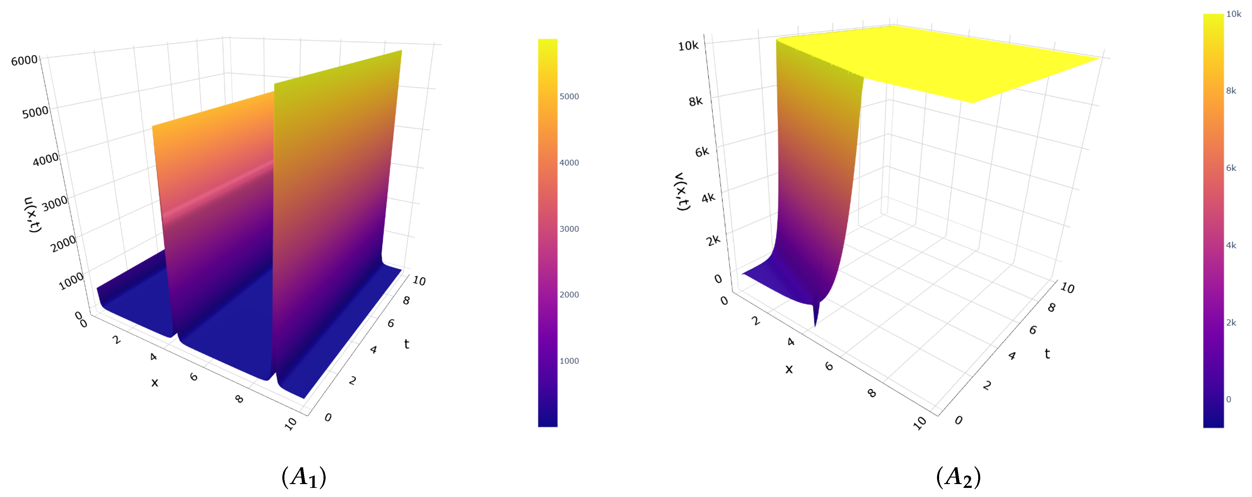
where $f_i(i=1,\dots ,4)$ are arbitrary constants. Here $\wp (z;g_2,g_3)$ denotes the Weierstrass elliptic function with invariants $(g_2,g_3)$. The graphs of the solution to (18) with $d_1=1$, $d_2=1$, $a=2,f_1=0,f_2=1,f_3=1$ and $f_4=-1$ are presented in Figure 3.

(4) Using operator (8), we construct a plane-wave ansatz

$$\begin{array}{c}\hfill u=U(w),v=V(w),w=x-\lambda t,\lambda \in \mathbb{R}.\end{array}$$

(19)

Using (19), we reduce the system (2) into following the system of ordinary differential equations

$$\begin{array}{cc}\hfill & d_1{U}^{″}+\lambda U^{\prime }-(a+k)U^2+2bV+cU-2kUV=0,\hfill \\ \hfill & d_2{V}^{″}+\lambda V^{\prime }+{\displaystyle \frac{a}{2}}{U}^2-bV=0.\hfill \end{array}$$

(20)

Since it is difficult to construct a general solution for the nonlinear system (20) with arbitrary coefficients, we try to find particular solutions of (20). Suppose that the following condition is satisfied:

$$\begin{array}{c}\hfill V={\beta }_0+{\beta }_{1}U,\end{array}$$

(21)

where ${\beta }_0$ and ${\beta }_1$ are constants to be determined. Substituting (21) into (20), we obtain an overdetermined system with nonzero solutions whose coefficients satisfy the following restrictions: $c=-3b$, $a=-2k$, ${\beta }_0=0$, ${\beta }_1=1$, $d_1=d_2=d$. So we have $U=V$ and the system (20) becomes the following case

$$\begin{array}{c}\hfill d{U}^{″}+\lambda U^{\prime }+U(-b-kU)=0.\end{array}$$

(22)

The nonlinear ordinary differential Equation (22) has been well studied because it is obtained by the reduction of the classical Fisher equation [10,24].

We can use the power series method [25,26] to solve this ordinary differential Equation (22). Let the solution of power series $U={\displaystyle \sum _{n=0}^{\infty }}{s}_n{w}^n$ and plug it into (22), where $s_n$$(n=0,1,\dots )$ are the undetermined coefficients. We can obtain

$$\begin{array}{c}\hfill d\sum _{n=0}^{\infty }(n+1)(n+2)s_{n+2}{w}^n+\lambda \sum _{n=0}^{\infty }(n+1)s_{n+1}{w}^n-b\sum _{n=0}^{\infty }{s}_n{w}^n-k\sum _{n=0}^{\infty }\sum _{m=0}^n{s}_{n-m}{s}_m{w}^n=0.\end{array}$$

(23)

For $n=0$, it is obtained from (23) that

$$\begin{array}{c}\hfill s_2={\displaystyle \frac{k{s_0}^2+b{s}_0-\lambda s_1}{2d}}.\end{array}$$

(24)

For $n\ge 1$, Equation (23) yields the following recurrence relation for $s_{n+2}$:

$$\begin{array}{c}\hfill s_{n+2}={\displaystyle \frac{b{s}_n-\lambda (n+1)s_{n+1}+k{\displaystyle \sum _{m=0}^n}{s}_{n-m}{s}_m}{d(n+1)(n+2)}},\end{array}$$

(25)

where ${\left\{s_n\right\}}^{\infty }$ is uniquely determined by (24). Substituting (24) and (25) into $U={\displaystyle \sum _{n=0}^{\infty }}{s}_n{w}^n$, we can obtain the solution of (22) as

$$\begin{array}{c}\hfill U=s_0+s_{1}w+{\displaystyle \frac{k{s_0}^2+b{s}_0-\lambda s_1}{2d}}{w}^2+\sum _{n=1}^{\infty }{\displaystyle \frac{b{s}_n+k{\displaystyle \sum _{m=0}^n}{s}_{n-m}{s}_m-\lambda (n+1)s_{n+1}}{d(n+1)(n+2)}}{w}^{n+2},\end{array}$$

(26)

where $s_n$ can be represented by $s_0,s_1$. So the solution of (2) is

$$\begin{array}{c}\hfill u=v=s_0+s_1(x-\lambda t)+{\displaystyle \frac{k{s_0}^2+b{s}_0-\lambda s_1}{2d}}{(x-\lambda t)}^2+\sum _{n=1}^{\infty }{\displaystyle \frac{b{s}_n+k{\displaystyle \sum _{m=0}^n}{s}_{n-m}{s}_m-\lambda (n+1)s_{n+1}}{d(n+1)(n+2)}}{(x-\lambda t)}^{n+2}.\end{array}$$

(27)

This solution can be used to simulate certain pathological interaction regimes between populations.

All parameter values are strictly selected to satisfy the existence and regularity conditions of system (2). For parameters with specific biological implications, their values are restricted to positive numbers to ensure the non-negativity of the solutions, consistent with the inherent constraints of physical quantities such as population densities and substance concentrations.

System (2) models the densities of isolated and paired Myxobacteria, denoted by $u(x,t)$ and $v(x,t)$, along a one-dimensional habitat. The exact solutions obtained provide analytically tractable spatiotemporal profiles that complement numerical simulations and facilitate qualitative understanding of the system’s behavior.

The solution families can be summarized as follows: exponential-type solutions capture early-time growth or decay regimes or local amplification behavior; hyperbolic-function solutions exhibit localized aggregation or depletion patterns, with characteristic widths determined by the balance between diffusion and reaction terms; elliptic-function solutions generate spatially periodic or quasi-periodic patterns, illustrating repeated aggregation structures; and traveling-wave solutions describe front-like propagation, connecting the isolated–paired model to classical invasion-front dynamics.

Overall, these exact solutions provide analytically tractable benchmarks for numerical validation, representative spatiotemporal patterns reflecting different dynamical behaviors, and insight into how parameter combinations affect the structure and evolution of the system. These results lay the foundation for subsequent derivation of conservation laws via Ibragimov’s method, which provide invariant diagnostics for further analytical and numerical investigations of system (2).

4. Conservation Laws

Conservation laws play an important role in physics and mathematical models. They not only provide an in-depth understanding of the dynamic behavior of systems but also provide important guidance for the solution of analytical solutions and the accuracy of numerical simulations. The conservation laws are determined by $D_t(C^t)+D_x(C^x)=0$, where $C=(C^t,C^x)$ is the conserved vector, and $D_i={\displaystyle \frac{\partial }{\partial x_i}}+u_i{\displaystyle \frac{\partial }{\partial u}}+v_i{\displaystyle \frac{\partial }{\partial v}}+u_{ij}{\displaystyle \frac{\partial }{\partial u_j}}+v_{ij}{\displaystyle \frac{\partial }{\partial v_j}}+\cdots$ is the total differentiation with respect to independent variables $x_i$. According to Ibragimov’s new conservation theorem [27], the conservation laws of the system (2) are constructed based on the adjoint equations and symmetries.

For equation $F(x,u,u_{(1)},\dots ,u_{(s)})=0$ with a finite number of variables $x=(x^1,\dots ,x^n)$, $u=(u^1,\dots ,u^m)$ and $u_{(s)}$ (s-derivative of u), the Lie point symmetry operator

$$X={\xi }^i(x,u){\displaystyle \frac{\partial }{\partial x^i}}+{\eta }^{\alpha }(x,u){\displaystyle \frac{\partial }{\partial u^{\alpha }}},i=1,\dots ,n,\alpha =1,\dots ,m$$

(28)

provides the conservation laws $D_i(C^i)=0$, where ${\xi }^i,{\eta }^{\alpha }$ are undetermined functions. The conservation vector is given by

$$C^i={\xi }^i\mathcal{L}+W^{\alpha }[{\displaystyle \frac{\partial }{\partial u_i^{\alpha }}}-D_j({\displaystyle \frac{\partial }{\partial u_{ij}^{\alpha }}})+D_j{D}_k({\displaystyle \frac{\partial }{\partial u_{ijk}^{\alpha }}})-\cdots ]+D_j(W^{\alpha })[{\displaystyle \frac{\partial }{\partial u_{ij}^{\alpha }}}-D_k({\displaystyle \frac{\partial }{\partial u_{ijk}^{\alpha }}})+\cdots ]+\cdots ,i=1,\dots ,n,$$

(29)

where $W^{\alpha }$ and $\mathcal{L}$ are defined as follows:

$$\begin{array}{cc}\hfill & W^{\alpha }={\eta }^{\alpha }-\sum _{j=1}^n{\xi }^j{u}_j^{\alpha },\alpha =1,\dots ,m,\hfill \\ \hfill & \mathcal{L}=\sum _{\beta =1}^m{\nu }^{\beta }{F}_{\beta }(x,u,u_{(1)},\dots ).\hfill \end{array}$$

(30)

Moreover, ${\nu }^{\beta }$ are new dependent variables satisfying the adjoint equations

$$F_{\alpha }^{*}={\displaystyle \frac{\partial {\displaystyle \sum _{\beta =1}^m}{\nu }^{\beta }{F}_{\beta }(x,u,u_{(1)},\dots )}{\partial u^{\alpha }}}+\sum _{k=1}^{\infty }{(-1)}^k{D}_{i_1}\cdots D_{i_k}{\displaystyle \frac{\partial {\displaystyle \sum _{\beta =1}^m}{\nu }^{\beta }{F}_{\beta }(x,u,u_{(1)},\dots )}{\partial u_{i_1\dots i_k}^{\alpha }}}=0,\alpha =1,\dots ,m.$$

(31)

For the system (2), let the Lagrangian be

$$\mathcal{L}=h(x,t)(d_1{u}_{xx}-a{u}^2+2bv+cu-k{u}^2-2kuv-u_t)+r(x,t)(d_1{u}_{xx}-a{u}^2+2bv+cu-k{u}^2-2kuv-v_t)$$

(32)

with four dependent variables $u(x,t),v(x,t),h(x,t),r(x,t)$.

The conserved vector of the infinitesimal generator $X_1+X_3$ in Case 1 is

$$\begin{array}{cc}\hfill & C^t=h(u-u_x)+r(v-v_x),\hfill \\ \hfill & C^x=h(u_t-d_1{u}_x-2bv-cu)+h_x(d_{1}u-d_1{u}_x)+r(v_t-d_2{v}_x+bv)+r_x(d_{2}v-d_2{v}_x).\hfill \end{array}$$

(33)

The conserved vector of the infinitesimal generator $X_1$ in Case 2 is

$$\begin{array}{ll}{C}^t=& -h(2t{d}_1{u}_{xx}+4btv+x{u}_x)-r(2t{d}_2{v}_{xx}+2v+x{v}_x),\\ C^x=& h(x{u}_t-2bxv+bxu+2b{d}_{1}t{u}_x+2t{d}_1{u}_{xt}+d_1{u}_x)-d_1{h}_x(2btu+2t{u}_t+x{u}_x)+\\ & r(x{v}_t+bxv+d_2{v}_x(2bt+3)+2d_{2}t{v}_{xt})-d_2{r}_x((2bt+2)v+2t{v}_t+x{v}_x).\end{array}$$

(34)

The conserved vector of the infinitesimal generator $X_2$ in Case 3 is

$$\begin{array}{l}{C}^t=h(2td{u}_{xx}+x{u}_x)+r(2td{v}_{xx}+x{v}_x),\\ C^x=h(2bxv+cxu-x{v}_t+2cdt{u}_x+4btd{v}_x-2dt{u}_{xt}-d{u}_x)+d{h}_x(2t{u}_t-2ctu-4btv+x{u}_x)\\ \hspace{1em}\hspace{1em}\hspace{1em}\hspace{1em}\hspace{1em}-r(x{v}_t+bxv+2btd{v}_x+d{v}_x+2dt{v}_{xt})-d{r}_x(2btv+2t{v}_t+x{v}_x).\end{array}$$

(35)

The conserved vector of the infinitesimal generator $X_1$ in Case 4 is

$$\begin{array}{l}{C}^t=h(-t{d}_1{u}_{xx}-ctu+kt{u}^2+2ktuv-u-{\displaystyle \frac{x}{2}}{u}_x)-r(t{d}_2{v}_{xx}+v+{\displaystyle \frac{x}{2}}{v}_x-{\displaystyle \frac{c}{2k}}),\\ C^x=h(d_{1}t{u}_{xt}+{\displaystyle \frac{3}{2}}{d}_1{u}_x+{\displaystyle \frac{x}{2}}{u}_t+kxuv+{\displaystyle \frac{x}{2}}k{u}^2-{\displaystyle \frac{x}{2}}cu)-d_1{h}_x(t{u}_t+u+{\displaystyle \frac{x}{2}}{u}_x)\\ \hspace{1em}\hspace{1em}\hspace{1em}\hspace{1em}+r({\displaystyle \frac{x}{2}}{v}_t+{\displaystyle \frac{3}{2}}{d}_2{v}_x+d_{2}t{v}_{xt})-d_2{r}_x(v-{\displaystyle \frac{c}{2k}}+t{v}_t+{\displaystyle \frac{x}{2}}{v}_x).\end{array}$$

(36)

The conserved vector of the infinitesimal generator $X_1$ in Case 5 is

$$\begin{array}{l}{C}^t=-h(d_{1}t{u}_{xx}+{\displaystyle \frac{x}{2}}{u}_x+u+ctu+2tuv)-r(d_{2}t{v}_{xx}+{\displaystyle \frac{x}{2}}{v}_x+v+{\displaystyle \frac{c}{2a}}+{\displaystyle \frac{a}{2}}t{u}^2),\\ C^x=h(d_{1}t{u}_{xt}+{\displaystyle \frac{3}{2}}{d}_1{u}_x+{\displaystyle \frac{x}{2}}{u}_t-xuv-{\displaystyle \frac{x}{2}}cu)-d_1{h}_x(t{u}_t+u+{\displaystyle \frac{x}{2}}{u}_x)\\ \hspace{1em}+r({\displaystyle \frac{x}{2}}{v}_t+{\displaystyle \frac{3}{2}}{d}_2{v}_x+d_{2}t{v}_{xt}-ax{u}^2)-d_2{r}_x(v+{\displaystyle \frac{c}{2a}}+t{v}_t+{\displaystyle \frac{x}{2}}{v}_x).\end{array}$$

(37)

The conservation laws derived in Section 4 reflect intrinsic invariance properties of system (2). While the system includes source and nonlinear interaction terms, these laws provide integral constraints under standard boundary conditions, which can be used to check the accuracy of numerical simulations, assist in symmetry reductions, and compare different parameter regimes. Combined with the exact solutions from Section 3, they offer analytic benchmarks and structured tools for analyzing the model’s dynamics.

5. Conclusions

In this paper, we analyzed a two-component reaction–diffusion system using Lie point and Q-conditional symmetries. The symmetry classification and reductions allowed us to derive exact solutions and simplified forms, providing an analytically tractable framework for understanding the system’s structure.

For the Myxobacteria isolated–paired interpretation, the classification identifies parameter regimes with additional symmetry structure, including cases where the dynamics reduce effectively to lower-dimensional forms. The explicit solutions illustrate four representative behaviors: (i) early-time growth/decay, (ii) localized aggregation/depletion patterns, (iii) spatially periodic structures via elliptic functions, and (iv) Fisher-type traveling fronts. These solutions serve as benchmarks for numerical validation and provide direct insight into how microscopic interactions influence macroscopic patterns.

Conservation laws derived using Ibragimov’s method complement the exact solutions, offering integral invariants that can be used to assess numerical schemes and explore parameter-dependent system behavior.

Overall, the combined analysis of symmetries, exact solutions, and conservation laws establishes a structured framework for studying coupled reaction–diffusion systems, and lays the foundation for future extensions to higher-dimensional or nonlocal models.

References

1. Ames, W.F. (Ed.) Nonlinear Partial Differential Equations in Engineering; Academic Press: Cambridge, MA, USA, 1965. [Google Scholar]
2. Murray, J.D. Mathematical Biology, 2nd ed.; Springer: Berlin/Heidelberg, Germany, 1993. [Google Scholar]
3. Simpson, M.J.; McCue, S.W. Reaction-diffusion models of biological invasion: Open source computational tools, key concepts, and analysis. arXiv 2024, arXiv:2403.01667. [Google Scholar]
4. Mastromatteo, I.; Toth, B.; Bouchaud, J.P. Anomalous Impact in Reaction-Diffusion Models. Phys. Rev. Lett. 2014, 113, 268701. [Google Scholar] [CrossRef] [PubMed]
5. Okubo, A.; Levin, S.A. Diffusion and Ecological Problems: Modern Perspectives; Springer: New York, NY, USA, 2001; Volume 14. [Google Scholar]
6. Lee, R. Reaction-Diffusion Equations in Spatial Ecology. Ph.D. Dissertation, The Ohio State University, Columbus, OH, USA, 2024. [Google Scholar]
7. Mahmud, A.A.; Tanriverdi, T.; Muhamad, K.A. Exact traveling wave solutions for (2+1)-dimensional Konopelchenko-Dubrovsky equation by using the hyperbolic trigonometric functions methods. Int. J. Math. Comput. Eng. 2023, 1, 11–24. [Google Scholar] [CrossRef]
8. Calvez, V.; El Abdouni, A.; Estavoyer, M.; Madrid, I.; Olivier, J.; Tournus, M. Regime switching on the propagation speed of traveling waves of some size-structured Myxobacteria population models. ESAIM Proc. Surv. 2024, 77, 195–212. [Google Scholar] [CrossRef]
9. Estavoyer, M.; Lepoutre, T. Traveling waves for a fast reaction limit of a discrete coagulation-fragmentation model with diffusion and proliferation. J. Math. Biol. 2024, 89, 2. [Google Scholar] [CrossRef] [PubMed]
10. Fisher, R.A. The wave of advance of advantageous genes. Ann. Eugen. 1937, 7, 355–369. [Google Scholar] [CrossRef]
11. Olver, P.J. Applications of Lie Groups to Differential Equations; Springer: New York, NY, USA, 1986. [Google Scholar]
12. Cherniha, R. Construction and application of exact solutions of the diffusive Lotka–Volterra system: A review and new results. Commun. Nonlinear Sci. Numer. Simul. 2022, 113, 106579. [Google Scholar] [CrossRef]
13. Dorodnitsyn, V.A.; Kaptsov, E.I.; Kozlov, R.V.; Meleshko, S.V. One-dimensional MHD flows with cylindrical symmetry: Lie symmetries and conservation laws. Int. J. Non-Linear Mech. 2023, 148, 104290. [Google Scholar] [CrossRef]
14. Bluman, G.W.; Cole, J.D. The general similarity solution of the heat equation. J. Math. Mech. 1969, 18, 1025–1042. [Google Scholar]
15. Olver, P.J.; Rosenau, P. The construction of special solutions to partial differential equations. Phys. Lett. A 1986, 114, 107–112. [Google Scholar] [CrossRef]
16. Olver, P.J.; Rosenau, P. Group-invariant solutions of differential equations. SIAM J. Appl. Math. 1987, 47, 263–278. [Google Scholar] [CrossRef]
17. Olver, P.J.; Vorob’ev, E.M. Nonclassical and conditional symmetries. In CRC Handbook of Lie Group Analysis of Differential Equations, Volume III: Theoretical Developments and Computational Methods; Ibragimov, N.H., Ed.; CRC Press: Boca Raton, FL, USA, 1996; pp. 291–328. [Google Scholar]
18. Clarkson, P.A.; Winternitz, P. Nonclassical symmetry reductions for the Kadomtsev–Petviashvili equation. Physica D 1991, 49, 257–272. [Google Scholar] [CrossRef]
19. Clarkson, P.A.; Winternitz, P. Symmetry reduction and exact solutions of nonlinear partial differential equations. In The Painlevé Property: One Century Later; Conte, R., Ed.; Springer: New York, NY, USA, 1999; pp. 591–660. [Google Scholar]
20. Cherniha, R.; King, J.R. The Shigesada–Kawasaki–Teramoto model: Conditional symmetries, exact solutions and their properties. Commun. Nonlinear Sci. Numer. Simul. 2023, 124, 107313. [Google Scholar] [CrossRef]
21. Cherniha, R.; Davydovych, V. New conditional symmetries and exact solutions of the diffusive two-component Lotka–Volterra system. Mathematics 2021, 9, 1984. [Google Scholar] [CrossRef]
22. Cherniha, R.; Davydovych, V. A Hunter-Gatherer–Farmer Population Model: New Conditional Symmetries and Exact Solutions with Biological Interpretation. Acta Appl. Math. 2022, 182, 4. [Google Scholar] [CrossRef]
23. Arrigo, D.J. Symmetry Analysis of Differential Equations: An Introduction; John Wiley & Sons: Hoboken, NJ, USA, 2015. [Google Scholar]
24. Ablowitz, M.J.; Zeppetella, A. Explicit solutions of Fisher’s equation for a special wave speed. Bull. Math. Biol. 1979, 41, 835–840. [Google Scholar] [CrossRef]
25. Morgan, A.P.; Sommese, A.J.; Wampler, C.W. A power series method for computing singular solutions to nonlinear analytic systems. Numer. Math. 1992, 63, 391–409. [Google Scholar] [CrossRef]
26. Algehyne, E.A.; El-Rahman, M.A.; Faridi, W.A.; Asjad, M.I.; Eldin, S.M. Lie point symmetry infinitesimals, optimal system, power series solution, and modulational gain spectrum to the mathematical Noyes–Field model of nonlinear homogeneous oscillatory Belousov–Zhabotinsky reaction. Results Phys. 2023, 44, 106123. [Google Scholar] [CrossRef]
27. Ibragimov, N.H. A new conservation theorem. J. Math. Anal. Appl. 2007, 333, 311–328. [Google Scholar] [CrossRef]
Figure 1. ( A 1 , A 2 ) are 3D plots of the solution in (14).
Mca 31 00022 g001
Figure 2. ( A 1 , A 2 ) are 3D plots of the solutions in (16).
Mca 31 00022 g002
Figure 3. ( A 1 , A 2 ) are 3D plots of the solutions in (18).
Mca 31 00022 g003