Optimization for Sustainability: A Comparative Analysis of Evolutionary Crossover Operators for the Traveling Salesman Problem (TSP) with a Case Study on Croatia

Abstract

This study presents a systematic comparison of five crossover operators used in genetic algorithms (GA) for the Traveling Salesman Problem (TSP). Partially Mapped Crossover (PMX), Order Crossover (OX), Cycle Crossover (CX), Edge Recombination (ERX), and Alternating Edges (AEX) are evaluated within an identical GA framework using tournament selection, inversion mutation, generational replacement, and elitism. Experiments were conducted on seven datasets, including three TSPLIB benchmarks, a clustered synthetic instance, a uniformly random instance, and two real-world Croatian city sets of 50 and 100 cities. Thirty independent GA runs per operator were analyzed using the Friedman test followed by Holm-corrected Wilcoxon pairwise comparisons. The Friedman test shows highly significant global performance differences. After applying Holm correction, the top four operators (PMX, OX, CX, and ERX) are statistically comparable on most datasets, as the correction eliminates most pairwise differences among them. All pairwise comparisons involving AEX remain significant across every dataset, confirming its consistently inferior performance. OX achieves the best average ranks across all datasets consistently, while PMX, CX, and ERX exhibit comparable mid-range performance. To illustrate practical relevance, optimized routes for Croatian instances were used to estimate fuel consumption and CO₂ emissions for petrol, diesel, and electric vehicles. The results demonstrate meaningful sustainability benefits achievable through optimized routing.

1. Introduction

The Traveling Salesman Problem (TSP) naturally occurs in different engineering disciplines. The basic problem formulation is simple: a person has a map of cities to visit, must visit each city exactly once before returning to the starting position, while minimizing the total distance traveled.

Efficient solutions to routing and combinatorial optimization problems such as the TSP underpin a wide range of applications in engineering design, robotics, logistics, and smart manufacturing [1,2,3,4]. By improving the robustness and convergence characteristics of evolutionary operators—resulting in shorter total traveling distances—the analysis presented here contributes to the development of optimization frameworks that support sustainable technological systems and intelligent decision-making.

Efficient TSP solvers have broader societal relevance, as they align with several United Nations Sustainable Development Goals (SDGs) [5]. Their impact extends beyond computational optimization into real-world sustainability challenges:

• SDG 3 (Good Health and Well-Being): Efficient routing contributes indirectly to improved public health by reducing vehicle emissions, noise pollution, and traffic congestion.
• SDG 9 (Industry, Innovation, and Infrastructure): Optimized routing enhances the efficiency of industrial and manufacturing systems, including automated guided vehicles (AGVs), robotic manipulators, and production logistics.
• SDG 11 (Sustainable Cities and Communities): In urban contexts, improved routing algorithms are applied to public transport scheduling, postal delivery, and waste collection.
• SDG 12 (Responsible Consumption and Production): Reduced travel distances translate directly into lower resource and energy consumption per delivered product.
• SDG 13 (Climate Action): Transportation is a significant contributor to greenhouse gas emissions. Even modest improvements in route efficiency, when applied across vehicle fleets, yield substantial reductions in CO₂ output.

Collectively, these outcomes demonstrate how algorithmic intelligence contributes to sustainable and resilient engineering solutions—bridging computational optimization with environmental and societal impact.

Despite the simplicity of the problem formulation, the solution to this problem is mathematically complex, since the problem is NP-hard [6]. This implies that computational effort to find an exact optimal solution grows factorially with the number of cities, n!. The consequence is that brute-force approaches to finding optimal solutions become infeasible for already moderately sized problem instances. Assuming 2 × 10⁹ ops/s, the time t for solving a 10-city instance requires microseconds, a 15-city instance seconds, and for 20 cities it is already measured in years. That is why alternative approaches to solving this problem are an important and active field of research and show that even advanced solvers struggle to scale well beyond tens of cities [7,8]. A well-known improvement over brute force is the Held–Karp dynamic programming algorithm [9], which substantially reduces the search effort compared to enumerating all possible tours. However, the time and memory required to store intermediate states in dynamic tables grow exponentially, which makes this algorithm typically applicable to smaller instances around 20–25 cities, on standard hardware [10,11,12]. Thus, although considerably more efficient than brute force, such exact approaches remain limited to small problem sizes.

This limitation motivates the development of advanced heuristic and metaheuristic approaches for solving the TSP and related combinatorial optimization problems, but also general high-dimensional optimization problems [13]. Among the most widely studied are Evolutionary Algorithms (EA) [14], Particle Swarm Optimization (PSO) [15], Ant Colony Optimization (ACO) [16] and Artificial Bee Colony (ABC) [17] algorithms, but also a combination of these algorithms [18]. In [19], the authors use rule-based mechanisms for the PSO algorithm to successfully solve problems of hundreds of nodes. A hybrid evolutionary algorithm is successfully used to solve multiple TSP and mTSP problems [20]. Ant Colony Optimization ACO algorithm is successfully applied to TSP with parameter tuning in [21,22]. Another swarm algorithm, ABC with local heuristic mechanisms, is successfully used for a variety of TSP instances of up to 64 cities in [23]. All these methods share similar characteristics—they employ nature-inspired algorithms based on the social behavior of biological organisms to solve a complex problem. Moreover, all these algorithms are so-called population-based algorithms. That means that they operate on populations of potential solutions, rather than a single solution, to explore the search space in a parallel manner [24].

Recent studies also highlight the importance of proper operator selection within evolutionary algorithms [25]. However, either small TSP instances or single-run results without rigorous statistical evaluation are usually reported. As a result, a fundamental question of how canonical crossover operators differ in convergence behavior, solution quality, and computational efficiency under controlled conditions remains insufficiently addressed.

These algorithms are heuristic, meaning they do not formally guarantee an optimal solution [26]. The quality of the solution depends, besides problem size, on the algorithm’s parameters. In terms of evolutionary algorithms (EAs), and in particular genetic algorithms (GAs), which are used in this study, these parameters are: the crossover operator and its probability, the mutation operator and its probability, and algorithm parameters such as population size and selection mechanism. When applied to TSP, the computational effort of GA is mainly related to the number of generations (or iterations) it executes, population size (number of candidate solutions evaluated per generation), and the cost of evaluating a single tour. This evaluation in symmetric TSP requires simply adding distances between consecutive cities. Thus, the work for processing a candidate solution grows proportionally with the number of cities. If population size and number of generations are fixed, or increase slowly, overall computational effort increases roughly proportionally with the number of cities. This represents a significant improvement compared to exhaustive or exact methods, where requirements grow factorially and become infeasible for moderately sized instances.

The important tradeoff is that heuristic algorithms, including GA, cannot guarantee global optimality. The main conclusion here is that EAs are applicable to large TSP instances, where exact methods are computationally infeasible. However, because of the heuristic nature, there is no guarantee that the absolute shortest route will be found. The good and practical fact is that even if the absolute shortest path is not found, a significantly better solution will almost certainly be found. Comparing this solution at the end of the evolutionary search to the best individual from the initial population clearly and measurably indicates the improvement the algorithm has made, despite it not being the best possible solution. In engineering applications, such tradeoffs are often entirely acceptable since high-quality solutions can be obtained at a realistic effort compared to the high cost of searching for the absolute optimum.

Despite extensive research on the Traveling Salesman Problem (TSP) and the broad use of evolutionary, as well as other, algorithms for its solution, a clear understanding of how different crossover operators affect convergence, solution quality, and computational efficiency under controlled conditions remains largely unanswered.

In this paper, we present a statistically controlled comparison of five canonical crossover operators across multiple datasets of different sizes, using 30 independent GA runs and nonparametric statistical testing (the Friedman test, and Wilcoxon with Holm correction). The analysis confirms measurable performance differences at the raw level, although after multiplicity correction, only AEX remains consistently distinguishable from the other operators. In addition, we demonstrate practical relevance by optimizing a real route for 50 and 100 Croatian cities and quantifying associated impacts on energy use and CO₂ emissions. The findings provide a rigorous comparative evaluation of crossover operators and highlight their broader relevance in the context of the UN Sustainable Development Goals.

2. Materials and Methods

A genetic algorithm is designed and implemented for finding solutions to a TSP problem with various numbers of cities, n. A representative sample of five canonical crossover operators, which are confirmed to perform well on TSP problems [27], is implemented and analyzed in terms of the number of operations required to find an optimal solution and convergence completeness for different problem sizes n. It is important that, besides the speed, the algorithm also has the capacity to consistently find optimal or near-optimal solutions. Premature convergence, or trapping in local minima, is a known problem, and those parameters, or combinations of parameters, which minimize it will be identified and preferred in algorithm design and implementation for the case studies on 50 and 100-city maps of Croatia.

2.1. Solution Encoding

For an example of nine cities, n = 9, an initial random population of size G is generated:

$$\mathrm{Population}=\begin{array}{c}1 3 5 2 4 6 7 9 8\\ 9 3 2 4 8 7 5 6 1\\ 7 9 8 2 5 6 3 1 4\\ 8 1 5 4 6 7 9 2\hspace{0.33em}3\\ \dots \\ 2 5 1 3 6 9 8 7 4\end{array}.$$

Dimensions of the Population are fixed during the evolutionary process, with the number of rows equal to G, which is for number of individuals, and the number of columns equals n, which is for number of cities.

2.2. Fitness Function

Fitness function must reward those individuals which results in shorter routes, and has the following form:

$$\mathrm{F}={\displaystyle \frac{1}{{\sum }_{i=1}^{n}d\left(c_i,c_{i+1}\right)}},$$

where n is the number of cities, $c_i$ is the i-th city in the tour, $c_{n+1}$ is defined as $c_1$ to complete the loop, and $d\left(c_i,c_{i+1}\right)$ is the distance between city $c_i$ and c_i+1. Shorter distances result in a higher fitness, aligning with the maximization nature of the genetic algorithm. Shorter routes with higher fitness are more likely to be selected into the Parents population and thus to transfer their traits to the newly created offspring.

2.3. Selection

In this paper, a tournament selection method is implemented [28]. This is consistent with recent EA applications to TSP [20,29,30,31]. It is a preferred choice for this example compared to standard roulette wheel selection to promote diversity and prevent premature convergence in the early evolutionary search stage. It also allows tunable selection pressure through the tournament size k. For smaller tournaments, selection pressure is lower, giving weaker individuals an increased chance of survival. In this paper, after initial experiments, a tournament of size k = 3 is selected and maintained throughout all evaluations. The procedure of the tournament selection is as follows: Randomly select k individuals and create a tournament. The best individual is directly selected as a parent. Repeat the tournament until the parents’ population is full, i.e., it has the same number of members as the previous population. In this paper, the dimension G is fixed at 200 individuals across all runs. In addition, elitism is also implemented in selection procedures to avoid the complete loss of the best-performing individuals. This means that several of the best individuals from the previous population can be guaranteed to be preserved and transferred to the parents’ population. In this study, one elite member is directly transferred to the next population, which ensures that the convergence function will be monotonous, but also promotes diversity. Namely, a higher number of elite individuals might compromise convergence at an early stage if a local optimum has highly attractive potential.

2.4. Crossover Operators

Five commonly used crossover operators suitable for combinatorial optimization are implemented and thoroughly analyzed. Recent studies indicate that hybridizing or combining crossover operators yields highly efficient GA-based solutions in real-world routing [32]. In the present study, the focus is on pure, controlled performance comparison of five canonical crossover operators. Simple crossover methods are not applicable here since they result in illegal offspring [33].

For example, a single-point crossover implementation to TSP, with Parent 1 given in bold, is illustrated here:

Parent 1: 1 2 3 4 * 5 6 7 8 9

Parent 2: 9 3 7 8 * 2 6 5 1 4

If a randomly chosen break point * is located after the fourth numeral in the above given strings, offspring would be as follows:

Offspring 1: 1 2 3 4 2 6 5 1 4

Offspring 2: 9 3 7 8 5 6 7 8 9

It is clear from the above example that single-point crossover results in illegal routes, offspring in evolutionary terminology, because some cities remain unvisited, while other cities are visited multiple times. This would very soon lead to a trivial solution. That is why specially tailored crossovers are developed for the combinatorial optimization domain. But the idea behind them is not only to create feasible solutions, but also to capture higher-order favorable mechanisms, such as link and edge preservation, for example. The idea is to transmit as much as possible of the information contained in the parents, with special emphasis on that which is shared between parents. If we consider what these solutions represent, and that is generally an order in which elements occur, or a set of moves linking pairs of elements, this motivation becomes clear. In other words, a crossover that would create feasible offspring, but at the same time destroying these higher-order requirements, is certainly inferior to those that do not.

2.4.1. Partially Mapped Crossover (PMX)

This is one of the most widely used operators for permutation encoding domains. It was first proposed by Goldberg and Lingle as a recombination operator for TSP [34]. The procedure is as follows: Two break points are randomly selected and marked with *, and the segment between them is copied from Parent 1 directly to Offspring 1. The rest of Offspring 1 is filled with elements from Parent 2, considering conflicts that occur through the mapping of corresponding elements between their position in Parent 1 and Parent 2, respectively. Bold entries are segments from Parent 1.

Parent 1:	[1 2 3 * 4 5 6 7 * 8 9]
Parent 2:	[9 3 7 * 8 2 6 5 * 1 4]
Offspring 1:	[9 3 2 4 5 6 7 1 8]
Offspring 2:	[1 7 3 8 2 6 5 4 9]

2.4.2. Order Crossover (OX)

The Order Crossover (OX) was designed by Davis for ordered-based permutation problems [35]. The procedure is as follows: 1. Two break points are randomly selected. Segment between the two break points from Parent 1 is copied to the first offspring. 2. Starting from the second break point in the second parent, the remaining unused numbers are copied into the first offspring so that they appear in the second parent, wrapping around at the end of the list. 3. The second offspring is created in an analogous manner, with the parents’ roles reversed.

Parent 1:	[1 2 3 * 4 5 6 7 * 8 9]
Parent 2:	[9 3 7 * 8 2 6 5 * 1 4]
Offspring 1:	[3 8 2 4 5 6 7 1 9]
Offspring 2:	[3 4 7 8 2 6 5 9 1]

2.4.3. Cycle Crossover (CX)

Cycle crossover (CX) [36] is concerned with preserving as much information as possible about the absolute position in which elements occur. This operator has the motivation to preserve the absolute position in which elements occur. It operates by dividing the elements into cycles. The procedure starts with the first position in Parent 1. From this position, the same position in Parent 2 is identified (in this moment, this is position 1 in the second parent). Now we find the value defined in this same position in Parent 1. This value is copied to Parent 1 and presents the start of the new cycle. This is repeated until all values are filled in Parent 1, and then for Parent 2 analogously.

Parent 1:	[1 2 3 4 5 6 7 8 9]
Parent 2:	[9 3 7 8 2 6 5 1 4]
Offspring 1:	[1 3 7 4 2 6 5 8 9]
Offspring 2:	[9 2 3 8 5 6 7 1 4]

2.4.4. Edge Recombination Crossover (ERX)

ERX is based on the idea that an offspring should be created as far as possible using only edges that are present in both parents [37]. In this operator, a list of neighbors must be created for each city. Offspring is created iteratively, starting from an arbitrarily selected node, in each step, the next node is selected between the neighbors of the current node. Preferred is the node with the fewest neighbors to promote diversity. If no neighbors are present, a randomly selected node is chosen. Bold entries in the offspring correspond to nodes selected via edges present in the first parent.

Parent 1:	[1 2 3 4 5 6 7 8 9]
Parent 2:	[9 3 7 8 2 6 5 1 4]
Offspring 1:	[1 5 4 9 3 2 6 7 8]
Offspring 2:	[9 8 7 3 2 6 5 1 4]

2.4.5. Alternating Edges Crossover (AEX)

The AEX operator interprets a chromosome as a directed cycle of arcs [38]. The child cycle is formed by choosing in alternation arcs from the first and from the second parent, with some additional random choices in case of infeasibility. For instance, let the two parents be:

Parent 1:	[5 1 7 8 4 9 6 2 3]
Parent 2:	[3 6 2 5 1 9 8 4 7]

Arc 5→1 from the first parent is selected as the starting arc. The first offspring has the following form: O1: 5 1 * * * * * * *. Next arc is taken from the second parent, which originates from 1, i.e., 1→9. The offspring now becomes: O1: 5 1 9 * * * * * *. Next is the arc from the first parent originating from 9, etc. If a choice of the arc is unfeasible since it is already contained in the offspring, pick the lowest index unused city. Ordinary procedure is resumed thereafter. At the end, offspring have the following form:

Offspring 1:	[5 1 9 6 2 3 4 7 8]
Offspring 2:	[5 1 7 3 6 2 4 9 8]

2.5. Mutation Operator

The mutation operator is a unary operator that perturbs a single individual to locally change its properties. Initially, two mutation operators were evaluated—simple mutation and inversion operator. The results indicated a strong outperformance of the inversion compared to simple mutation; thus, simple mutation was omitted from further analysis. This complies with other relevant studies, which indicate that inversion mutation is the preferred choice for symmetric TSP problems [39]. Simple mutation selects a random city and inserts it after another random city: 1 2 3 4 5 6 7 8 9→if City 3 is randomly selected and City 6 randomly selected as point of insertion, mutated individual is: 1 2 4 5 6 3 7 8 9. Simple mutation yields feasible but small local changes, requiring many generations to achieve high-quality solutions.

Inversion operator selects two random cities in the individual and swaps the order of cities between the two: 1 2 3 4 5 6 7 8 9→if randomly selected cities were 4 and 7, with the segment 4 5 6 7 between them, then the mutated individual has the following form: 1 2 3 7 6 5 4 8 9.

3. Implementation of Genetic Algorithm

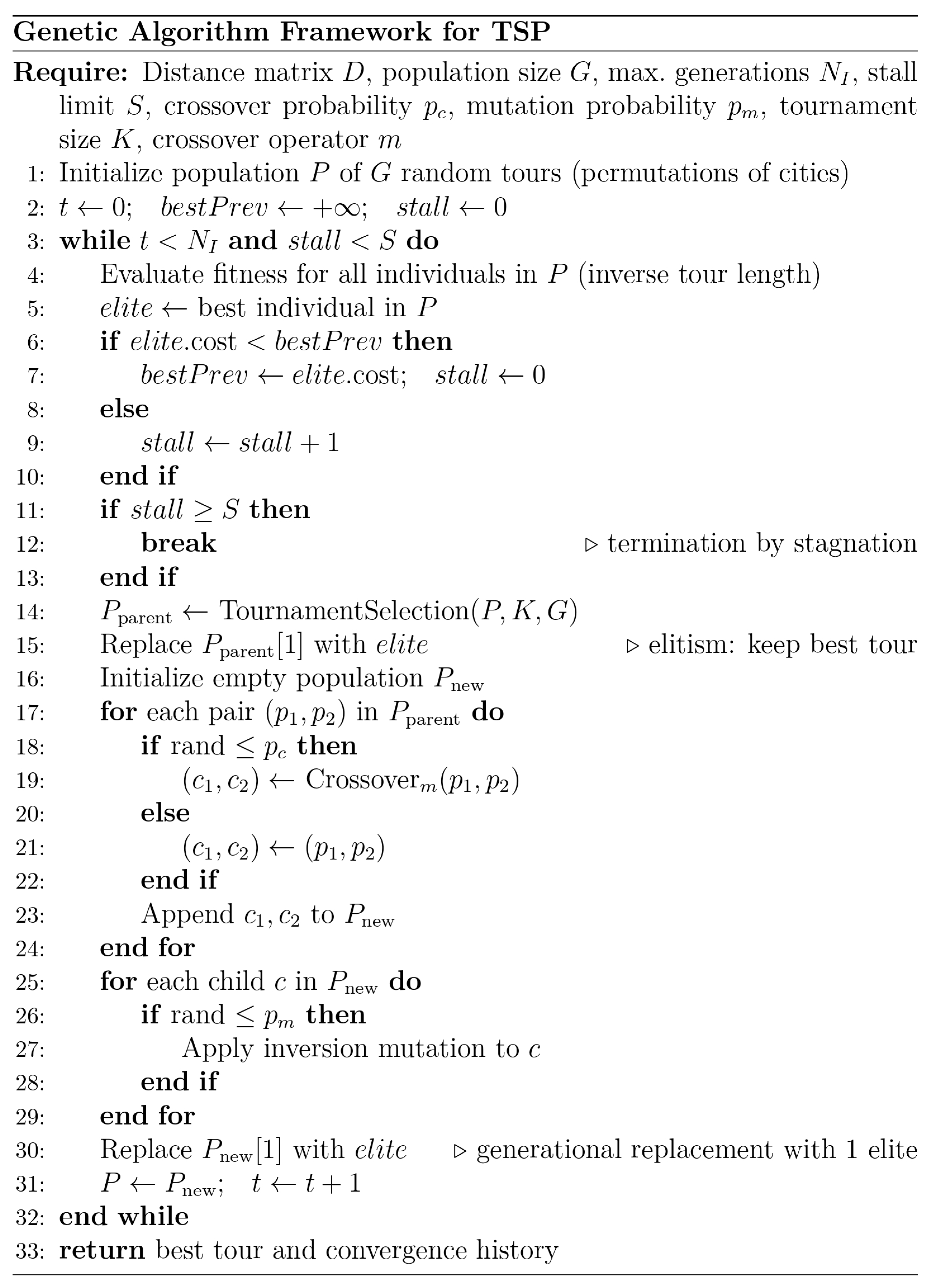
An initial parameter sweep is performed on a randomly generated TSP map with 50 uniformly distributed nodes. The motivation for this preliminary step is to identify favorable combinations of mutation probability, crossover probability, and population size across all crossover operators. Such values, if they exist, would later be used as a fixed baseline for comparative testing of the five crossover operators. The main algorithmic procedure of the Genetic algorithm used in this study is given in Figure 1.

The genetic algorithm (GA) employs tournament selection of size k = 3 with one elite member, which ensures monotonic improvement of the fitness function. For the exploratory sweep step, exhaustive search over the parameter space is performed with the following parameters: $p_c\in \left[0.4:0.1:0.9,\hspace{0.17em}0.95\right], { p}_m\in \left[0:0.1:0.8\right],$ Increments were defined as 0.1 for crossover and mutation sweep grid. In the case of crossover, there is an additional 0.95 value with half the step to test also for very high crossover rates. Population sizes were discretized and evaluated in the set: $\mathrm{G} \in \{50, 100, 150, 200\}.$ The algorithm was run for N_I = 5000 (hard limit) generations, with an early stopping criterion (stall limit) if no improvement occurred over the last S = 500 generations. Each configuration was repeated 10 times to increase the representativeness of the results. This setup is computationally very demanding, as the total number of runs grows rapidly due to the combinatorial expansion of tested parameter configurations. For this reason, population sizes greater than 200 individuals were not considered, as they would be computationally prohibitive within the scope of this study. Moreover, as shown in Section 4, a population of 200 individuals already provides sufficient diversity for the best-performing operators to reach near-optimal solutions within an acceptable runtime.

Table 1. Results of sweep step for optimal parameters per crossover operator. These are minima of mean length for each operator across the complete search space. Bold values indicate the best result (minimum) among all operators for each metric.

Operator	G	pc	pm	Avg. Best Len	Std. Best Len	Avg. Time (s)
PMX	200	0.9	0.6	5728	97	2.05
OX	200	0.7	0.4	5672	52	2.11
CX	200	0.8	0.7	5682	62	0.80
ERX	200	0.6	0.7	5688	80	3.19
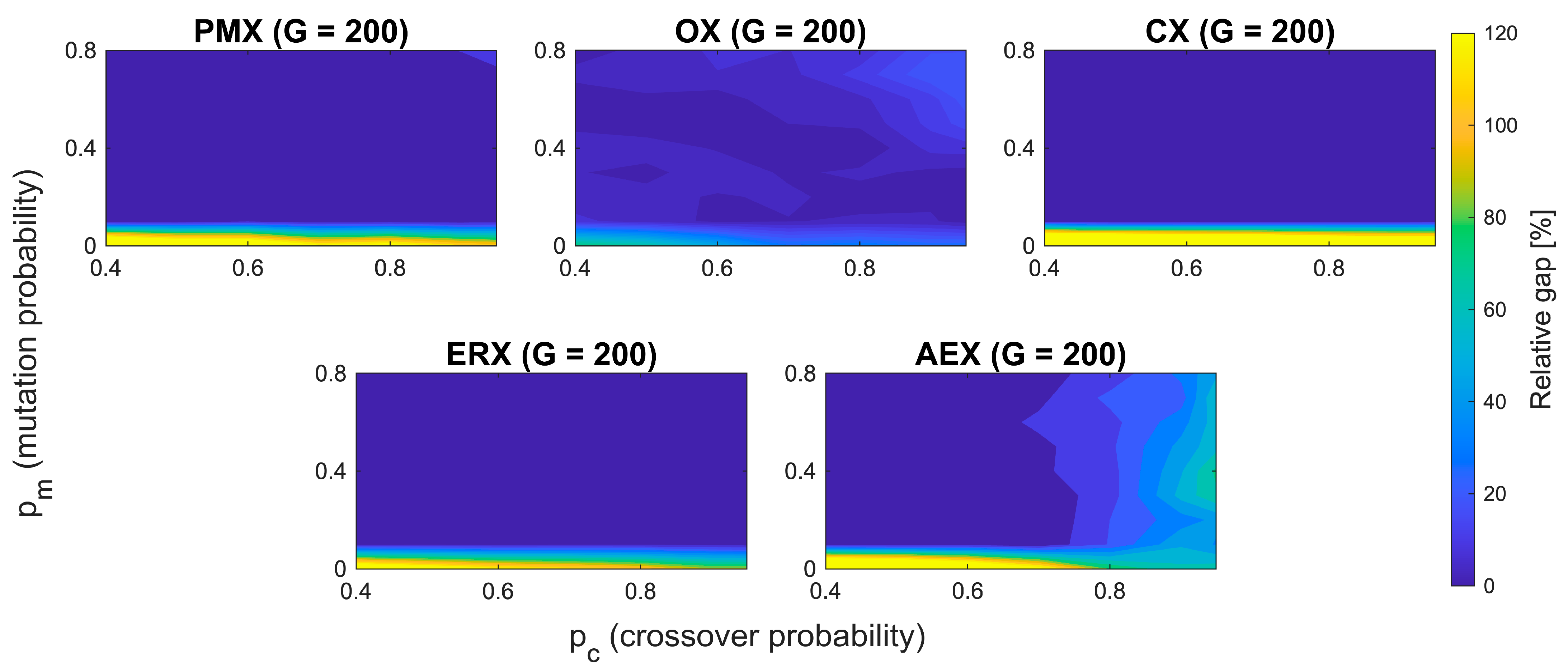
AEX	200	0.7	0.4	5790	139	7.49

summarizes the results of the parameter sweep step, reporting for each operator the combination of parameters with the lowest average tour length across the entire search space. These optimal configurations are also given in Figure 2.

Complete parameter landscape plots with top 10% contour regions are provided in Figures S1–S5. For consistency, only the best-performing configurations per operator are given in Table 1. All the operators show decreasing optimality gap for increased population sizes, except for PMX, which shows similar results for 150 and 200 population sizes. All the operators except AEX show a stable basin of performance across a relatively large range of mutation and crossover probabilities (large top 10% contour regions—Figures S1–S5). AEX has, on the contrary, a different behavior. Firstly, it shows a low sensitivity on population size, with decreasing optimality gap only marginally as population increases. Second, sharp boundaries are present, causing sudden changes from good to bad—for example, across the crossover probability of ~0.85, where a slight increase in p_c degrades performance. Similar holds for mutation probability, where a horizontal flat segment around p_m ~ 0.1 indicates high sensitivity at this value. Compared to other operators, AEX shows much more unpredictable behavior and sensitivity, which leads to fragility with respect to both parameters p_m and p_c.

To quantify the sensitivity of the AEX operator under its best achievable performance, for each of the 7 × 9 (p_c, p_m) parameter combinations, the shortest tour length across defined four population sizes (50, 100, 150, and 200) was identified. The standard deviation was afterwards computed across the 63 best achieved values. For AEX, calculated variability is $\mathsf{\sigma } = 2668$, which is approximately 3.27 times larger than the corresponding value for OX $\mathsf{\sigma } = 817$. In terms of variance, this indicates that AEX is an order of magnitude ≈ 10.7 times less stable than OX, confirming its fragility to parameter settings even in its best configurations. Based on these insights, a shared region is identified that provides consistently good performance across all the operators.

Although AEX shows fragmented behavior, the remaining operators (PMX, OX, CX, ERX) all share broad and stable region p_m ≈ [0.4, 0.7] and p_c ≈ [0.6, 0.9]. To ensure comparability across operators and to avoid regions that cause clearly unstable behavior in AEX, a common agreement is made on parameters such as p_m = 0.4, p_c = 0.7, and G = 200. For every operator, this parameter combination lies within its own top 10% performance region. This means that each operator is evaluated under settings which are close to its own best performing region, without giving bias to any parameter. The relative gap is calculated as follows:

$$\mathrm{R}\mathrm{e}\mathrm{l}\mathrm{a}\mathrm{t}\mathrm{i}\mathrm{v}\mathrm{e} \mathrm{G}\mathrm{a}\mathrm{p} \left(p_c,p_m,G\right)=\hspace{0.17em}{\displaystyle \frac{\overline{L}\left(p_c,p_m,G\right)-L_{min}}{L_{min}}} 100\left[\%\right],$$

where $\overline{L}$ is for the mean best route length obtained over ten independent runs for a given combination of p_c and p_m, and population size G. L_min is the minimum mean tour length achieved across all tested parameter combinations for the same crossover operator and population size (not exact TSP route optimum). Runtime was measured, and it scales approximately linearly with population size. Average values across all combinations of p_m and p_c, all crossover operators mean runtime per run was approximately: 0.92 s (G = 50), 1.81 s (G = 100), 2.68 s (G = 150) and 3.13 s (G = 200). Detailed run times are given in the following sections per operator and per map.

Operators CX, PMX, and OX are the fastest because they rely on simple positional and mapping operations. ERX is slower since it must maintain adjacency lists during recombination, but it remains competitive in terms of run time to CX, PMX, and OX. The AEX is significantly slower, typically 2 to 4 times slower across all experiments, compared to other operators. This underperformance, both in terms of solution quality and run time efficiency, can be linked to its alternating edge construction mechanism. AEX switches between parents’ edges in every step, thus frequently proposing edges that lead to cities already included in the partially constructed tour. This repeatedly triggers the procedure, which replaces the proposed edge with the lowest-indexed unvisited city. The consequence here is that a large fraction of edges in the offspring are not inherited from parents but inserted as the lowest index unvisited city. This has a disruptive effect and destroys repeatedly useful information from parents. It hinders the exploitation of quality links from parents and brings excessive randomness into the offspring. As a consequence, this operator shows higher variance, slower convergence, and less efficient runtime than the other four operators.

4. Results

To provide a consistent and reproducible experimental environment, each crossover operator was first evaluated on three standard benchmark problems from TSPLIB. Berlin 52, kroA100, and pr124 are used as the benchmarks. These maps present different layouts and impose potentially different requirements for the optimization algorithm. Berlin52 [40] is built upon actual 52 locations in the city of Berlin, with geometric layout forming several local groupings, kroA100 [41] is a highly irregular synthetic instance with mixed densities, while pr124 has a striped structure with linear elongated clusters. All the following experiments use the same GA configuration identified in the sweep step: G = 200, p_c = 0.7, p_m = 0.4, N_I = 5000, and stall limit S = 500.

Random seed was fixed with MATLAB’s rng(1) to ensure reproducibility and repeatability of results. This enables other researchers to reproduce the same experimental conditions and validate the findings. All simulations were executed on a workstation equipped with an Apple M1 Silicon processor (8-core CPU, 3.2 GHz maximum clock frequency, 8 GB unified RAM) running macOS 15.6.1. The algorithms were implemented in MATLAB Version 24.1.0.253703 (R2024a), utilizing the Optimization Toolbox (v24.1) for the mixed-integer linear programming solver (intlinprog) and the Statistics and Machine Learning Toolbox (v24.1) for hypothesis testing.

The relative optimality gap is calculated to compare the solutions found by each operator to the known solution from the TSP library. In the case of randomly generated maps, for smaller problems, intlinprog solver built into MATLAB can be used to calculate optimal solutions. This solver implements a proprietary mixed-integer linear programming (MILP) engine using branch-and-bound with linear programming (LP) relaxations. It is guaranteed to return a globally optimal solution only when the optimality gap is closed, i.e., when AbsoluteGap = U − L ≤ AbsoluteGapTolerance; where U and L are the solver’s upper and lower bounds. In our experiment, AbsoluteGapTolerance was set to 10⁻⁶, and the Croatia 50-city case reached a final optimality gap of 0, confirming that the returned tour is globally optimal. Larger instances (typically ≥ 100 cities) become computationally intractable for MILP under standard constraints and are therefore not solved exactly in this study.

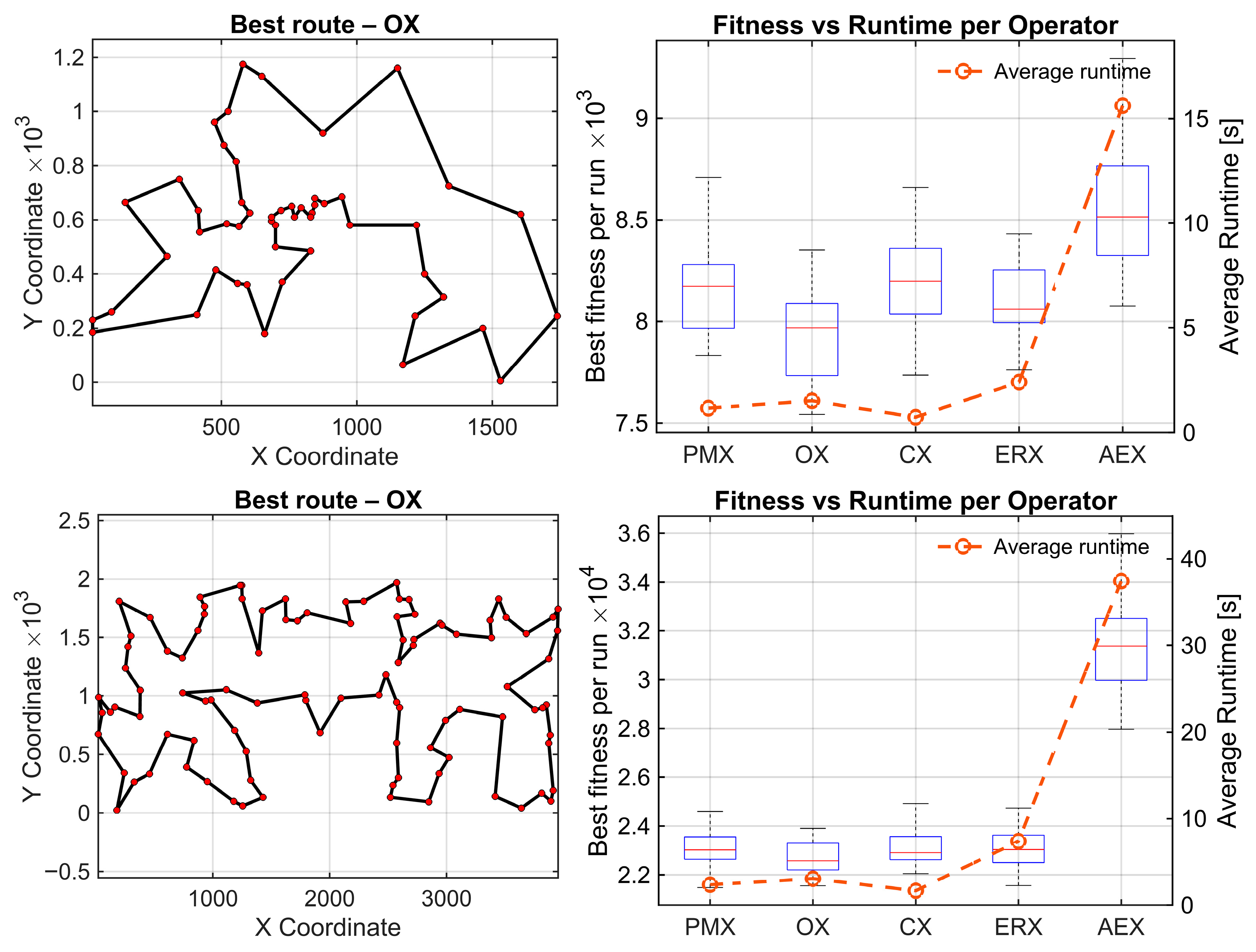
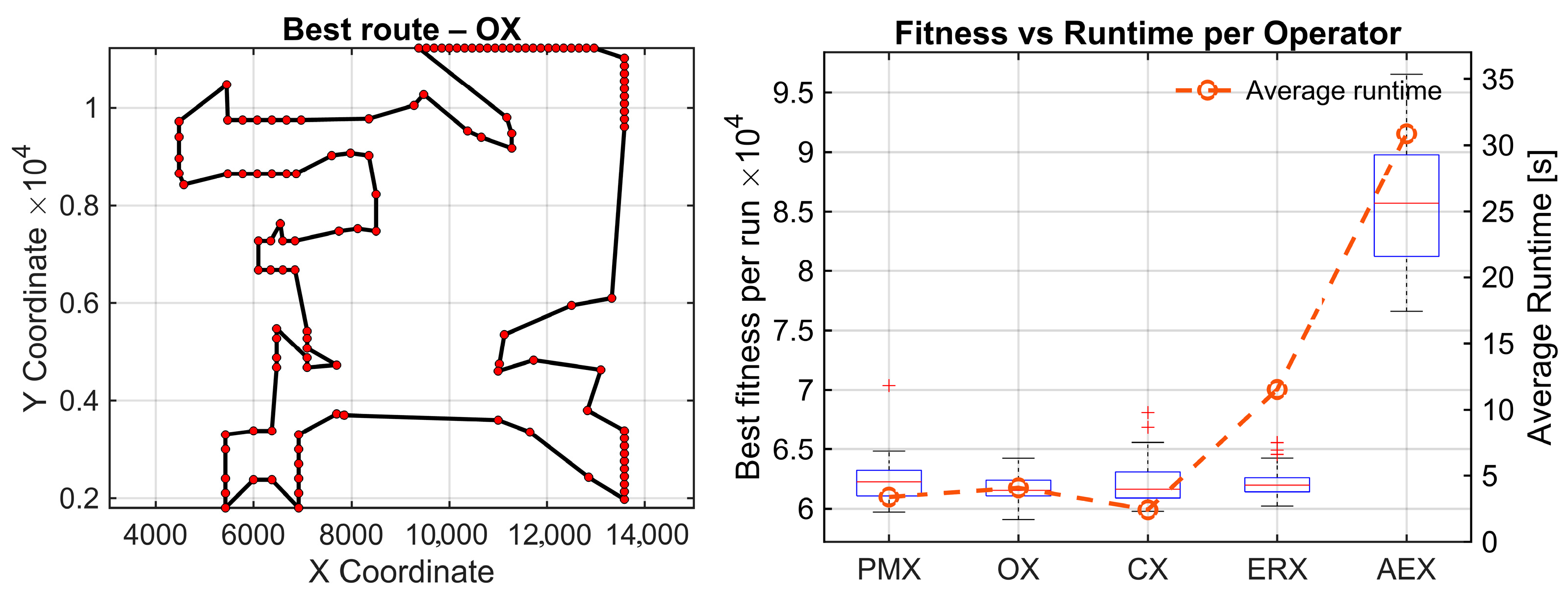
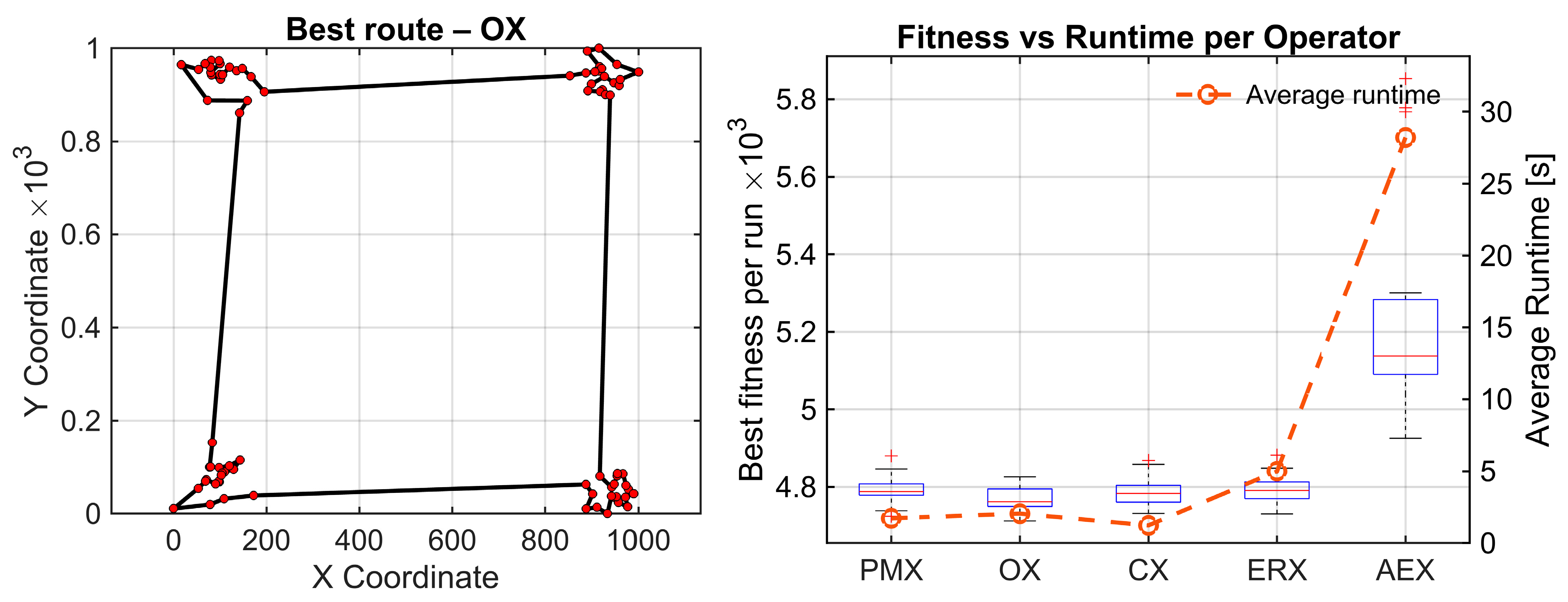
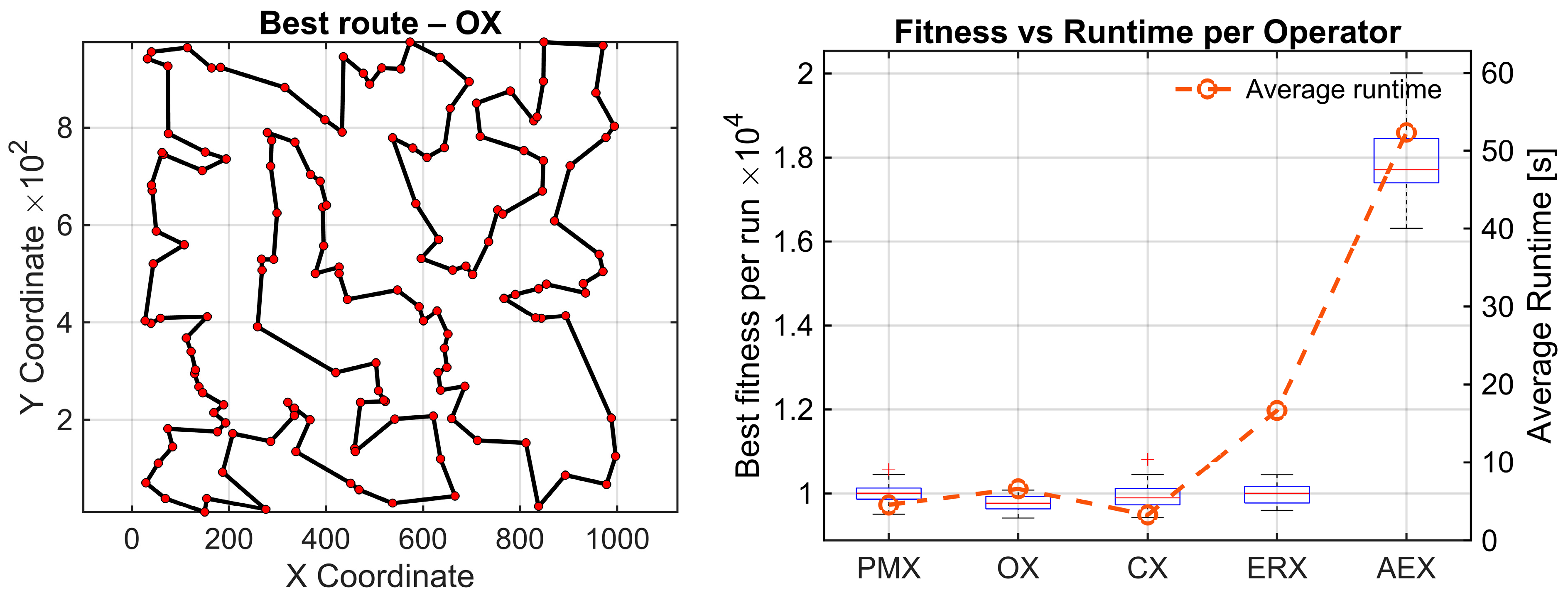
Results for these three benchmark maps are presented in Figure 3. On the left side, the best route found by the statistically best-performing operator for each benchmark is shown. The right side shows box plots summarizing the distribution of shortest routes across 30 independent runs for each crossover operator. The average runtime for every operator is also given for all operators for one full evolutionary run. This is the mean wall-clock time required per operator to execute one complete evolutionary run—all the generations averaged over 30 independent runs. To investigate statistical significance of differences within results for each parameter, statistical analysis is performed using the Friedman test and Wilcoxon post-hoc pairwise comparisons with Holm correction. The use of the Friedman test is validated by performing the Shapiro–Wilk test on paired performance differences for berlin52.tsp. Normality is violated in most comparisons (9 of 10 pairs with $p<{10}^{-7}$)$.$ Based on these results, the parametric ANOVA assumptions are not met, so the Friedman test followed by Holm-corrected Wilcoxon signed-rank test is appropriate. The algorithm runs 5000 generations and evaluates each of the five operators 30 times to get statistically representative samples.

To formally compare the crossover operators, the Friedman test was applied to the berlin52, kroA100, and pr124 benchmarks (n = 52, 100, and 124 nodes, respectively). For each map and each operator, the final tour length obtained at the end of the GA run served as the performance metric. Lower tour lengths indicate better solution quality. The Friedman test does not operate on raw values but on ranks. Thus, for each benchmark, the operators were ranked from best to worst based on their tour lengths, with Rank 1 corresponding to the best (shortest) route and Rank 5 to the worst (longest). These rank matrices constitute the input to the Friedman test.

For all the examples, the degree of freedom equals 4. On berlin52, the Friedman test detected a highly significant overall performance difference among five crossover operators (χ²(4) = 52.81, p = 9.3 × 10⁻¹¹), with a medium–strong effect size (Kendall’s W = 0.440). OX achieved the best average rank (1.60), while AEX was consistently the worst (4.50). Raw Wilcoxon signed-rank tests indicate several moderate differences among the best performing operators (e.g., PMX–OX: p = 7.15 × 10⁻⁴, OX–CX: p = 4.44 × 10⁻⁵, OX–ERX: p = 7.27 × 10⁻³, CX–ERX: p = 0.0368). All comparisons against AEX show extremely strong raw effects, with p-values between 1.73 × 10⁻⁶ and 4.86 × 10⁻⁵. After applying Holm’s step-down correction, all AEX-related comparisons remain statistically significant (p_Holm between 1.73 × 10⁻⁵ and 3.26 × 10⁻⁴). In this dataset, also PMX-OX, OX-CX, and OX-ERX comparisons remain significant. Remaining mid-range comparisons (PMX-CX, PMX-ERX, CX-ERX) become nonsignificant.

For kroA100, the Friedman test again reports highly significant overall differences (χ²(4) = 62.95, p = 6.95 × 10⁻¹³), with a strong effect size (Kendall’s W = 0.525). Average ranks show the four stronger operators form a group (OX = 2.12, ERX = 2.50, CX = 2.60, PMX = 2.78), whereas AEX is clearly weakest (avg. rank = 5.00). Raw Wilcoxon results reveal moderate p-values among the stronger operators (e.g., PMX–OX: 0.035, OX–CX: 0.047, OX–ERX: 0.082), while all comparisons involving AEX report extremely small p-values (1.73 × 10⁻⁶ in every AEX-related pair). After applying Holm correction, all AEX-related comparisons remain statistically significant (p_Holm ≈ 1.73 × 10⁻⁵), confirming AEX performs significantly worse than the remaining operators. None of the pairwise comparisons among PMX, OX, CX, and ERX remain statistically and significantly different after correction. Consequently, AEX is the only operator that clearly differs from the rest, whereas no statistically reliable differences appear among PMX, OX, CX, and ERX.

On pr124, the Friedman test once more confirms significant operator differences (χ²(4) = 61.95, p = 1.13 × 10⁻¹²) with a strong effect (Kendall’s W = 0.516). Average ranks again show a compact group of four strong operators (OX = 2.23, CX = 2.40, ERX = 2.60, PMX = 2.77) and a clearly inferior AEX (5.00).

Raw Wilcoxon comparisons among the stronger operators yield only mild or nonsignificant p-values (e.g., PMX–OX: 0.213, OX–ERX: 0.131, CX–ERX: 0.572), whereas all AEX-related comparisons again produce identical extremely small values (p = 1.73 × 10⁻⁶). After Holm correction, the four AEX-related comparisons remain significant (p_Holm ≈ 1.73 × 10⁻⁵). All other pairs remain nonsignificant, meaning that these operators form a compact, highly performing group and cannot be statistically separated on the pr124 dataset.

Performance results on the three TSPLIB benchmarks are summarized in

Table 2. Summary of performance per crossover operator for 3 TSPLIB benchmark instances. Bold values indicate the best result (minimum) among all operators for each metric.

berlin52–TSPLIB Optimum = 7524
Operator	Avg Best	Std Best	Best Run	Gap (Best) [%]	Avg Time [s]	Std Time [s]
PMX	8165	229	7832	3.85	1.1	0.3
OX	7929	254	7542	0.00	1.5	0.4
CX	8194	220	7734	2.55	0.7	0.1
ERX	8107	191	7760	2.89	2.4	0.3
AEX	8570	294	8075	7.07	15.6	3.4
kroA100–TSPLIB Optimum = 21,282
PMX	23,096	773	21,477	0.92	2.4	0.4
OX	22,710	660	21,549	1.25	3.1	0.5
CX	23,132	676	22,049	3.60	1.7	0.1
ERX	23,078	736	21,557	1.29	7.4	0.8
AEX	31,384	1807	27,971	31.43	37.4	0.7
pr124–TSPLIB Optimum = 59,030
PMX	62,393	1986	59,724	1.18	3.4	0.6
OX	61,708	1266	59,092	0.10	4.1	0.7
CX	62,186	2028	59,790	1.29	2.4	0.3
ERX	62,250	1358	60,228	2.03	11.5	1.2
AEX	85,773	5597	76,598	29.76	30.9	11.5

, which shows that OX achieves the lowest average route lengths, whereas AEX consistently yields the largest optimality gaps and longest runtimes.

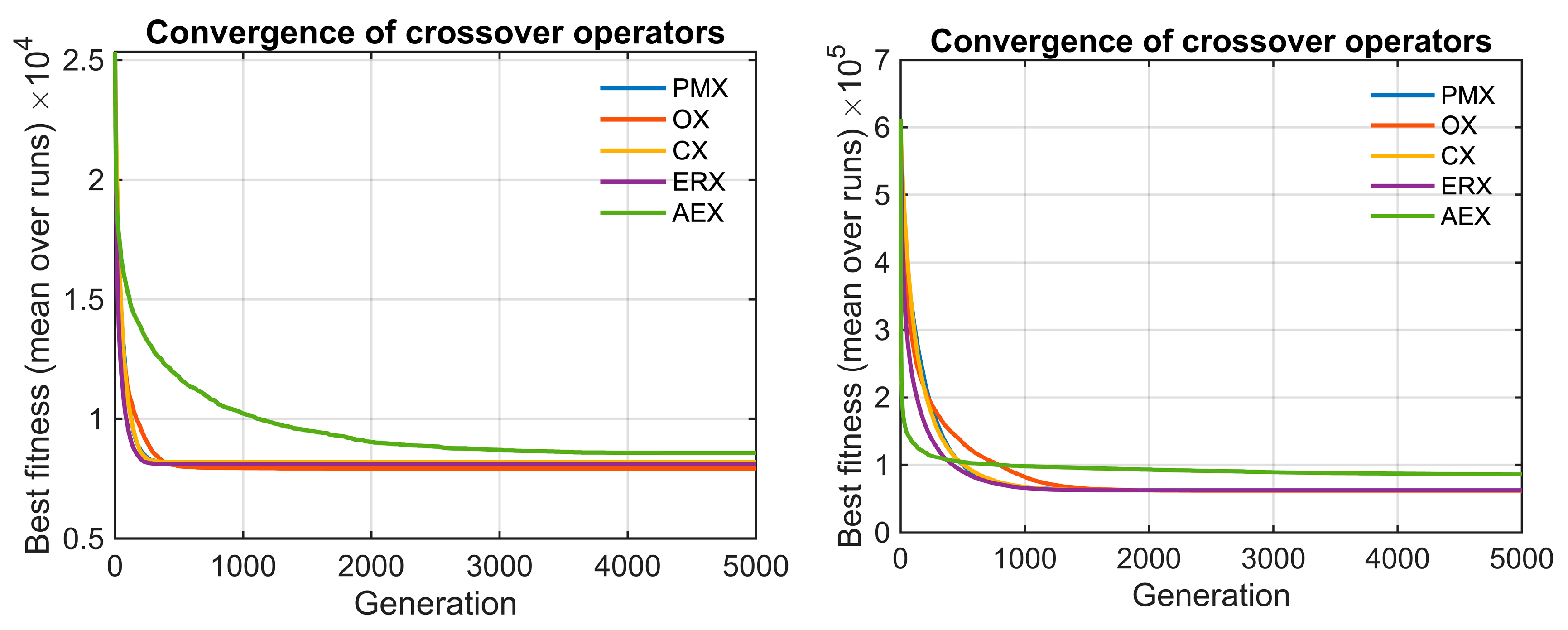
The convergence behavior of the crossover operators is presented in Figure 4 for berlin52 and pr124 instances. AEX consistently stagnates and fails to improve over generations, while the remaining operators converge very fast toward near-optimal solution quality. To verify whether similar performance patterns exist also under different spatial structures and problem sizes, we additionally evaluated the operators on two synthetically generated maps. We created two instances: C4x20.tsp, consisting of four clusters with 20 nodes in each, and random150.tsp with 150 uniformly distributed nodes. Parameters of the genetic algorithm were kept identical to those used on previously described benchmarks.

The clustered C4x20 instance produced a highly significant Friedman test again (χ²(4) = 63.91, p = 4.36 × 10⁻¹³), with a strong effect size (Kendall’s W = 0.533). The average ranks show a compact cluster of strong operators (OX = 2.03, ERX = 2.58, CX = 2.67, PMX = 2.72), while AEX is clearly inferior with a rank of 5.00. The Holm-corrected Wilcoxon pairwise comparisons indicate that none of the top four operators differ significantly from the other.

The only reliable signal is that AEX is consistently inferior, because all raw comparisons between AEX and every other operator are extremely small $p_{\mathrm{raw}}\approx 1.7\times {10}^{-6}$, and effect sizes are large (r = −0.87). All AEX-related differences remain significant after Holm correction (p_Holm ≈ 1.73 × 10⁻⁵), confirming its inferiority.

The random 150 instances yield the strongest statistical contrast for all the analyzed datasets. The Friedman test reports (χ²(4) = 67.81, p = 6.57 × 10⁻¹⁴), with the highest effect size observed in this study (Kendall’s W = 0.565). Again, four operators form a tight top group (OX = 1.87, CX = 2.43, ERX = 2.83, PMX = 2.87), whereas AEX remains the clear outlier with an average rank of 5.00. All comparisons related to AEX remain statistically significant after Holm correction (p_Holm ≈ 1.73 × 10⁻⁵) with very large effect sizes (r = −0.87). This confirms AEX is inferior to all other operators in this instance. For this dataset, significant differences remain after Holm correction between OX-PMX $p_{\mathrm{Holm}}=0.0058$, effect size r = 0.60, and OX-ERX, $p_{\mathrm{Holm}}=0.0121$, and r = 0.55. Other differences remain nonsignificant. The results of these experiments are given in Figure 5.

Based on this strict statistical interpretation, the combined evidence across datasets analyzed in this study allows us to identify OX as the best-performing operator. This conclusion is based on the global pattern of average ranks and the consistency of performance across a complete set of heterogeneous maps. On every dataset, OX attains the best, or second-best, average rank. Other operators (PMX, CX, and ERX) either alternate between strong and moderate performance, indicating no stable dominance. Thus, although the Holm-corrected post-hoc tests do not statistically confirm that OX outperforms PMX, CX, or ERX, the practical evidence and ranking stability consistently point to OX as the most reliable and best-performing operator across the analyzed benchmark instances. Effect sizes $\mathrm{r}=\mathrm{z}/\sqrt{n}$ They are used to further clarify the practical importance of statistical data. Comparisons of OX vs. PMX/CX/ERX show medium effect sizes ($\left|r\right|\approx 0.3-0.5$) across datasets consistently in favor of OX. Comparison of OX vs. AEX shows very large effects ($\mathrm{r}\approx -0.87)$ uniformly over all datasets. Comparisons among PMX, CX, and ERX yield a small ($\left|r\right|\left(<0.2\right)$) effect, indicating negligible practical differences within operators that form the middle-performing group.

AEX is the only operator that is inferior to others. Its average ranks are consistently the lowest (rank 5.00 across all datasets, and 4.50 on berlin52), and the paired Wilcoxon tests yield very small p-values and large effect sizes, indicating a large and systematic performance deficit. After applying the Holm correction, all AEX related comparisons remain highly significant, confirming AEX is inferior to all other crossover operators across all datasets. All statistical results are provided in Tables S2–S21.

To apply the presented algorithm to a real-world case, two original datasets for Croatia were created. An instance of 50 and 100 Croatian cities, respectively. These are fully TSPLIB-compliant datasets provided in EUC2D and GEO systems and generated to sample cities uniformly from all regions of Croatia. The benchmark datasets used in this research have been deposited in the Zenodo repository and are freely accessible under the MIT License: https://doi.org/10.5281/zenodo.17587540.

For each city, geographic coordinates (latitude and longitude) were obtained from publicly available open data sets. Since the coordinates were in decimal degrees, using the World Geodetic System 1984 (WGS84) datum, the haversine formula is used to convert to pairwise distances that account for Earth’s curvature. For conversion details, please refer to Equations (S1)–(S4).

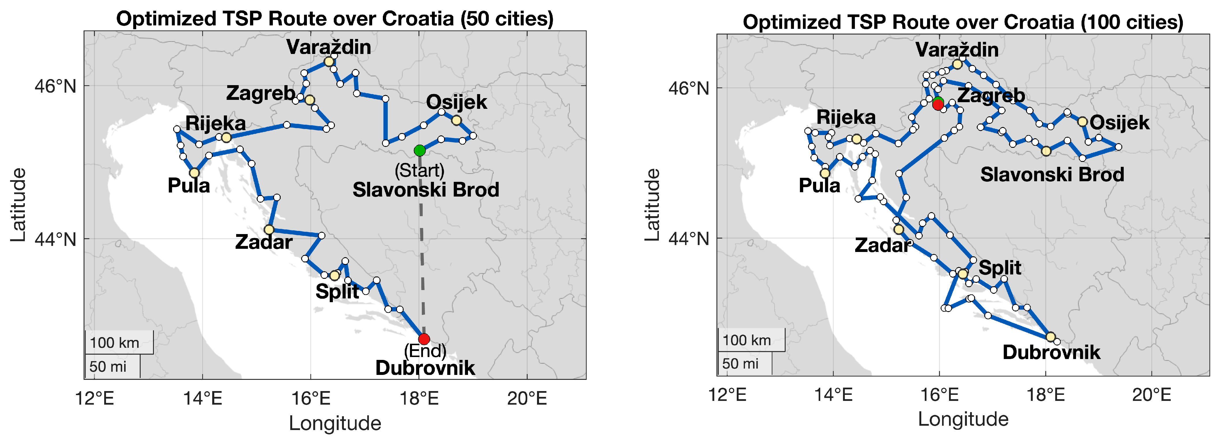
Then the resulting distance matrix was used as input to the TSP algorithm using solely the OX operator, which was identified as the best performing operator in the tested benchmark sets. The algorithm was run for 5000 generations, and successfully found the optimal route presented on the left side of Figure 6. The length of this route is ~1822 km, which is confirmed by the intlinprog function to be optimal. The same algorithm with identical parameters is then applied to the 100-city map in Croatia, as illustrated on the right side. Although the resulting route (~2465 km) is not guaranteed to be globally optimal, it represents a substantial improvement compared to the initial random population solution and demonstrates the scalability and practical utility of evolutionary crossover operators for realistic routing scenarios. This result also motivates further exploration of potential environmental benefits enabled by route optimization techniques.

To illustrate the environmental impact of optimized and unoptimized routes, transparent simplifications are adopted. Distances are piecewise linear segments without considering actual road layout, curvature, elevation differences, or traffic conditions. This allows us to assess differences only because of routing efficiency. This is a standard approach in exploratory sustainability assessments.

Three vehicle types are analyzed: (1) a petrol passenger car, (2) a diesel passenger car, and (3) a battery electric vehicle (BEV). For petrol and diesel, we use the Tier 1 CO₂ emission factors reported in the EMEP/EEA Air Pollutant Emission Inventory Guidebook [42] (Figure S6) combined with the typical fuel-consumption values for passenger cars from (Figure S7) (61.9 g/km for petrol and 56.8 g/km for diesel). Using the corresponding fuel densities (0.750 kg/L for petrol and 0.840 kg/L for diesel), these values convert to volumetric fuel consumption of 8.25 L/100 km for petrol and 6.76 L/100 km for diesel, and to distance-based CO₂ intensities of 196 g/km for petrol and 181 g/km for diesel. For the BEV, we assume an energy use of 21 kWh/100 km [43], representative of mid-sized BEVs, and apply the 2024 Croatian grid emission factor of 165 g CO₂/kWh [44], yielding a BEV carbon intensity of 34.7 g/km. Details on conversion are provided in Equations (S5)–(S19) in Supplementary Materials.

Under these assumptions, the optimal 1822 km route results in approximately 357 kg CO₂ for petrol, 329 kg CO₂ for diesel, and 63 kg CO₂ for the BEV. Because energy use per kilometer is assumed to be constant, emissions scale linearly with route length. Therefore, a route that is 5.91 times longer produces emissions approximately 5.91 times higher. The same proportionality applies to the 100-city instance.

5. Discussion

The extensive evaluation across multiple datasets provides a coherent picture of how canonical operators behave within a GA framework used across TSP instances in this study. The general pattern emerges that OX, PMX, CX, and ERX form a group of well-performing operators, while AEX is isolated as an underperformer. This is reflected both with average ranks and Wilcoxon statistics, where AEX shows an extremely large performance deficit relative to all the other operators.

An important outcome from this study is the distinction between the raw performance differences and statistically reliable differences after multiplicity correction. On most datasets, several raw pairwise comparisons among the best-performing operators yield moderately small p-values, but they do not survive Holm correction, which is the consequence of the conservative nature of the procedure. However, on the berlin52 and random150 datasets, performance gaps among the strongest operators are large enough and remain statistically significant after Holm correction. This means that sufficiently large effect sizes will cause statistically reliable differences to remain detected. The only consistent pattern across all datasets is related to AEX. Comparisons of AEX with every other operator show extremely small raw p-values with very large effect sizes before and after Holm correction. This allows us to mark AEX as the inferior operator across all instances.

Another important observation is that the operators behave stably across problem sizes and spatial structures. Although effect sizes (Kendall’s W) increase slightly for larger maps, the separation pattern does not change—OX maintains the most favorable average rank, AEX remains inferior, and PMX/CX/ERX fluctuate within a narrow performance window. This suggests that the operators’ structural properties, rather than the TSP instance, are responsible for their relative effectiveness. OX benefits from its ability to preserve relative orderings of cities, which appears to generalize well across different geometries. AEX’s alternating-edge mechanism systematically destroys too many useful adjacencies, which renders it the lowest rank.

Average rank stability across all datasets makes OX the most reliable choice. Even if Holm-corrected tests can not declare it statistically superior to PMX, ERX, or CX on most datasets, the empirical evidence consistently places OX at or near the top across all experiments. AEX is, in contrast, both statistically and practically inferior.

Finally, the example of application to real Croatian routing instances illustrates how algorithmic improvements translate into real-world sustainability impacts. Even modest reductions in route length led to meaningful reductions in fuel consumption, travel time, and CO₂ emissions. This demonstrates a broader societal relevance of efficient evolutionary operators and links combinatorial optimization to multiple United Nations Sustainable Development Goals.

6. Conclusions

This study provides a rigorous and statistically controlled comparison of five canonical crossover operators in a GA-based TSP solver across heterogeneous datasets. The results consistently identify AEX as the clearly inferior operator. OX, PMX, CX and ERX form a stable group of competitive performers. Although raw statistics reveal moderate differences among the top four operators, most of these do not remain significant after Holm correction. This reveals the importance of robust statistical methodology when evaluating evolutionary operators. Among the competitive operators, OX exhibits the most stable performance across all map instances, making it the most reliable practical choice for general-purpose TSP optimization.

The real-world Croatian cases demonstrate that improvements in algorithm performance, and consequently in route efficiency, translate into meaningful reductions in fuel use, emissions, and other travel-related impacts. Thus, route optimization contributes to several UN Sustainable Development Goals by enabling cleaner, safer, and more resource-oriented transport systems.

Future research should investigate operator behavior across a broader dataset. Hybridization of operators, adaptive operator selection mechanisms, and a more exhaustive initial parameter sweep step across different TSP instances may offer additional insight into algorithmic robustness. Finally, integrating realistic traffic patterns and road models would further enhance the environmental relevance and practical impact of evolutionary-based route optimization.