Abstract
This study presents a low-cost and scalable CO2 monitoring system that leverages NDIR sensors and a Long Short-Term Memory (LSTM) neural network to predict indoor CO2 concentrations over both short- and long-term horizons. The proposed system aims to anticipate air quality deterioration in shared spaces, enabling proactive ventilation strategies. Various LSTM configurations were evaluated, optimizing the number of layers, neurons per layer, and input delays to enhance forecasting accuracy. The optimal model consisted of two LSTM layers with 128 neurons each and a time window of 10 previous observations. This model achieved an RMSE of approximately 57 ppm for an 8 h forecast in a classroom setting. Experimental results demonstrate the reliability of the proposed approach for CO2 prediction and its potential impact on indoor air quality management.
1. Introduction
In indoor environments, avoiding high concentrations of aerosols (microscopic particles exhaled when speaking or breathing) is critical, as these can degrade air quality and increase health risks. Poorly ventilated closed spaces exacerbate this issue, as the accumulation of aerosols and CO2 rises with the number of occupants and the time spent in such environments [1]. This situation is common in classrooms during face-to-face sessions, where ventilation is often insufficient to maintain moderate CO2 levels. Continuous CO2 monitoring is essential to assess air quality, along with predicting or forecasting CO2 concentration over time. This allows us to estimate how long it will take for a given space to reach CO2 levels that could pose a significant risk, enabling proactive air quality management.
The clean air we breathe “outdoors”, without pollution, contains approximately 400 parts per million (ppm) of CO2. In the literature, minimum reference levels are reported between 412 ppm and 420 ppm, according to various sources [2]. Air with this concentration of CO2 is considered to not have been breathed recently. CO2 concentrations above the reference level indicate that the air has already been partially exhaled by someone, as shown in Table 1. For instance, when the CO2 concentration reaches 1000 ppm, it is estimated that approximately 1.5% of the air has already been previously exhaled. Concentrations above 1000 ppm not only reflect reduced air quality but also pose a potential health risk, as elevated CO2 levels can be toxic [3,4].

Table 1.
Relationship between CO2 concentration and the fraction of breathed air †.
To assess air quality, the appropriate sensor must be selected. NDIR (non-dispersive infrared) sensors are suitable for measuring the concentration of CO2 since the molecules of this gas are prone to absorbing infrared light. Evaluations have already been made of NDIR sensors as a low-cost option for CO2 measurement. One of these was performed in a laboratory environment, demonstrating that, without any calibration or correction, NDIR sensors achieve RMS errors between 5 ppm and 21 ppm compared to a precision sensor [6]. CO2 measurements can be managed and analyzed by various methods. Typically, as a complement to monitoring systems, diagnosis/prognosis applications are developed where the data are processed through specialized programs (e.g., MATLAB) or cloud computing services, such as ThingSpeak, Microsoft Azure, and Amazon Web Services, among others [7]. Cloud computing offers data storage and analysis services to forecast various physical variables using computational intelligence techniques like neural networks. In Robin et al. [8], convolutional neural networks were evaluated to monitor air quality; on the other hand, Altikat et al. [9] also used neural networks to predict the passage of CO2 from the ground to the atmosphere. Recently, Kapoor et al. [10] designed a pilot monitoring system for CO2 using neural networks and support vector machines. However, real-time CO2 monitoring alone is insufficient for effective air quality management. Predictive modeling is necessary to estimate future CO2 concentrations and optimize ventilation strategies.
Monitoring CO2 levels is essential for ensuring indoor air quality (IAQ) and occupant well-being. Kwon et al. [11] classify CO2 sensors into two main types: chemical sensors, which are energy-efficient and compact but suffer from short lifespan and low durability, and non-dispersive infrared (NDIR) sensors, which offer higher accuracy and are commonly used for air quality monitoring. The integration of Internet of Things (IoT) technologies has significantly improved CO2 monitoring by enabling real-time data acquisition and remote accessibility. Marques and Pitarma [12] introduced iAQ WiFi, an IoT-based system that collects environmental data using low-cost sensors and transmits them via WiFi for real-time visualization and analysis. Marques et al. [13] expanded on this work with iAir CO2, an advanced IoT solution designed for continuous CO2 monitoring. Their study emphasizes the importance of real-time air quality tracking to anticipate and mitigate potential health risks.
Machine learning techniques have also been applied to CO2 forecasting, allowing for more efficient and proactive air quality management. Kallio et al. [14] investigated multiple machine learning models, including ridge regression, decision trees, random forest, and multilayer perceptron, to predict indoor CO2 concentration. Arsiwala et al. [15] developed a digital twin system integrating IoT, artificial intelligence, and Building Information Modeling (BIM) to automate CO2 emissions tracking. Alsamrai et al. [16] provided a comprehensive review of IoT-based air quality monitoring systems, emphasizing the growing use of low-cost sensors and microcontrollers such as ESP8266 and ESP32. Their findings confirm that IoT applications offer a cost-effective and scalable alternative for pollution monitoring.
Building upon these advancements, this study integrates predictive modeling and real-time data collection to enhance CO2 monitoring solutions. By leveraging machine learning and IoT technologies, our approach improves forecasting accuracy, supports proactive air quality management, and contributes to healthier indoor environments.
This study proposes an IoT-based CO2 monitoring and forecasting system, integrating low-cost monitoring stations equipped with NDIR sensors and ESP32 microcontrollers to provide real-time CO2 measurements. These devices are strategically deployed in classrooms, offices, and laboratories within Tecnológico Nacional de México campus Tuxtla Gutiérrez. The collected CO2 data are processed using an LSTM autoregressive neural network, trained to predict future CO2 concentrations up to eight hours in advance. Unlike traditional mathematical forecasting models, this approach allows the neural network to learn patterns directly from sensor data, enhancing adaptability to different environmental conditions. The results of this study suggest an alternative for scheduling classroom sessions to ensure safe air quality conditions. The main contributions of this study are summarized as follows:
- The LSTM network analyzes historical data to accurately forecast CO2 levels up to four hours in advance, eliminating the need for explicit models.
- A network of affordable sensors and wireless transmitters enables cost-effective deployment and easy maintenance, making the system highly scalable.
- Predictive insights allow proactive ventilation control, improving air quality, health, and cognitive performance in indoor environments.
- Real-time monitoring and forecasting optimize space utilization and enhance safety in educational institutions, supporting data-driven decision making.
The remainder of this document is organized as follows: Section 2 presents the materials and methods used for the monitoring system and the configuration of the LSTM network for CO2 concentration forecasting. Section 3 describes the results obtained in different configurations and the comparison with different methods reported in the literature. Finally, Section 4 presents the conclusions.
2. Materials and Methods
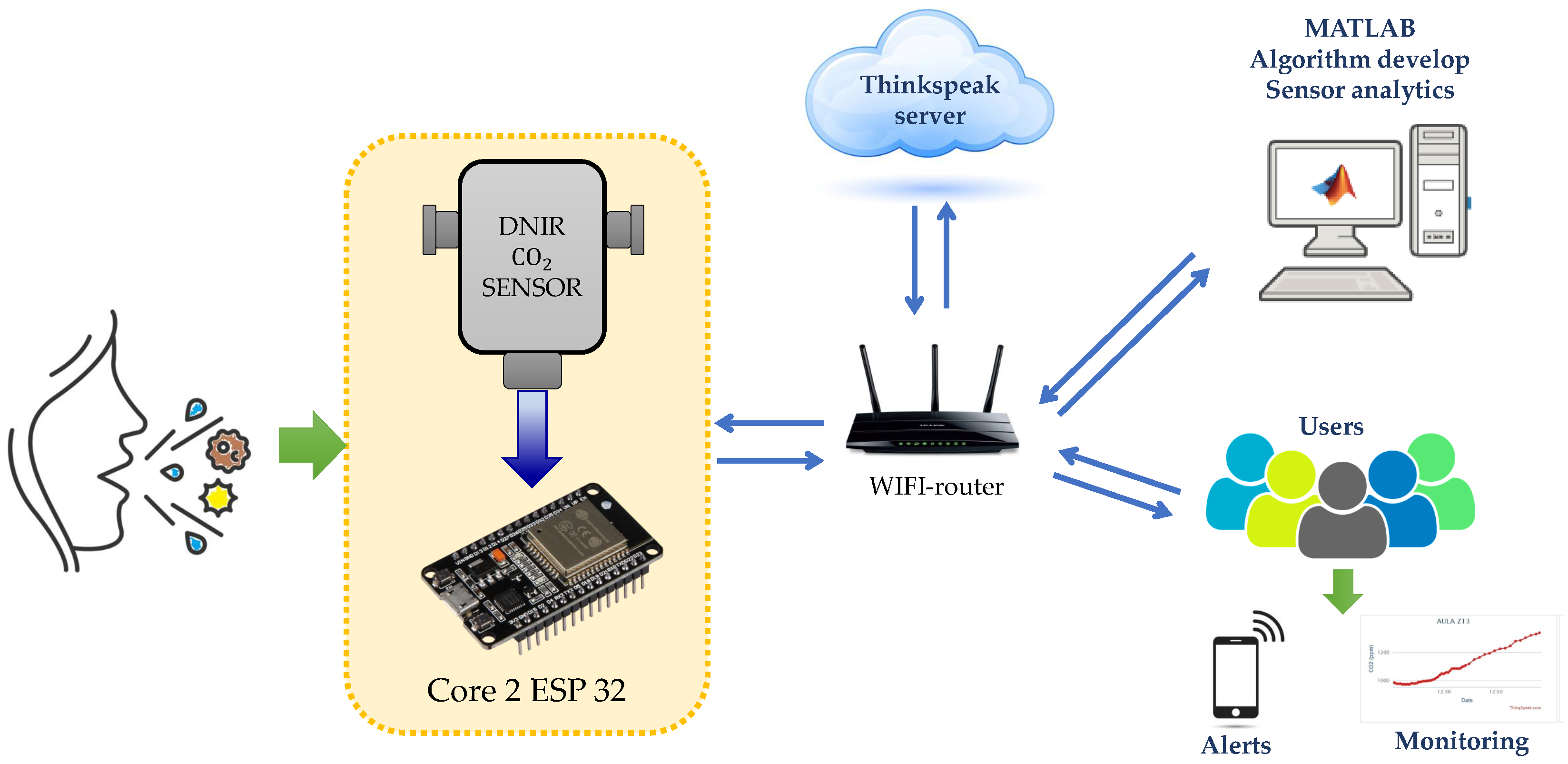
The CO2 monitoring system to prevent COVID-19 infection involves using an NDIR sensor and an ESP32-Core2 microcontroller board to monitor CO2 levels in indoor environments, as seen in Figure 1. The DNIR sensor is a kind of optical sensor that can detect the concentration of CO2 in the air by measuring light absorption at a specific wavelength.
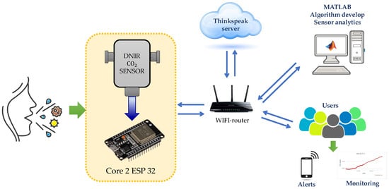
Figure 1.
General schema of the proposed methodology.
The ESP32-Core2 microcontroller board reads data from the DNIR sensor and sends them to the Thinhspeak cloud using WiFi connectivity. Thinhspeak is an IoT platform that provides data storage, analysis, and visualization tools. The collected CO2 data are then analyzed in Matlab, a popular data analysis and modeling tool. Using these data, a CO2 level prediction algorithm can be developed, which can estimate the CO2 level in the near future based on current measurements.
The CO2 level prediction algorithm based on LSTM results can be displayed to users on their mobile devices using an application. The application can show real-time monitoring graphs and alert users if the CO2 level exceeds a certain threshold, indicating that the indoor environment may be poorly ventilated and potentially hazardous to human health.
This system has the potential to prevent the spread of airborne diseases, such as COVID-19, by providing a tool for monitoring indoor air quality and identifying poorly ventilated environments that could increase the risk of pathogen transmission. The following sections describe the method in detail, including device connections for collecting sensor data, the neural network used, the training process, and the tested configurations.
2.1. Measurement of CO2 Concentration
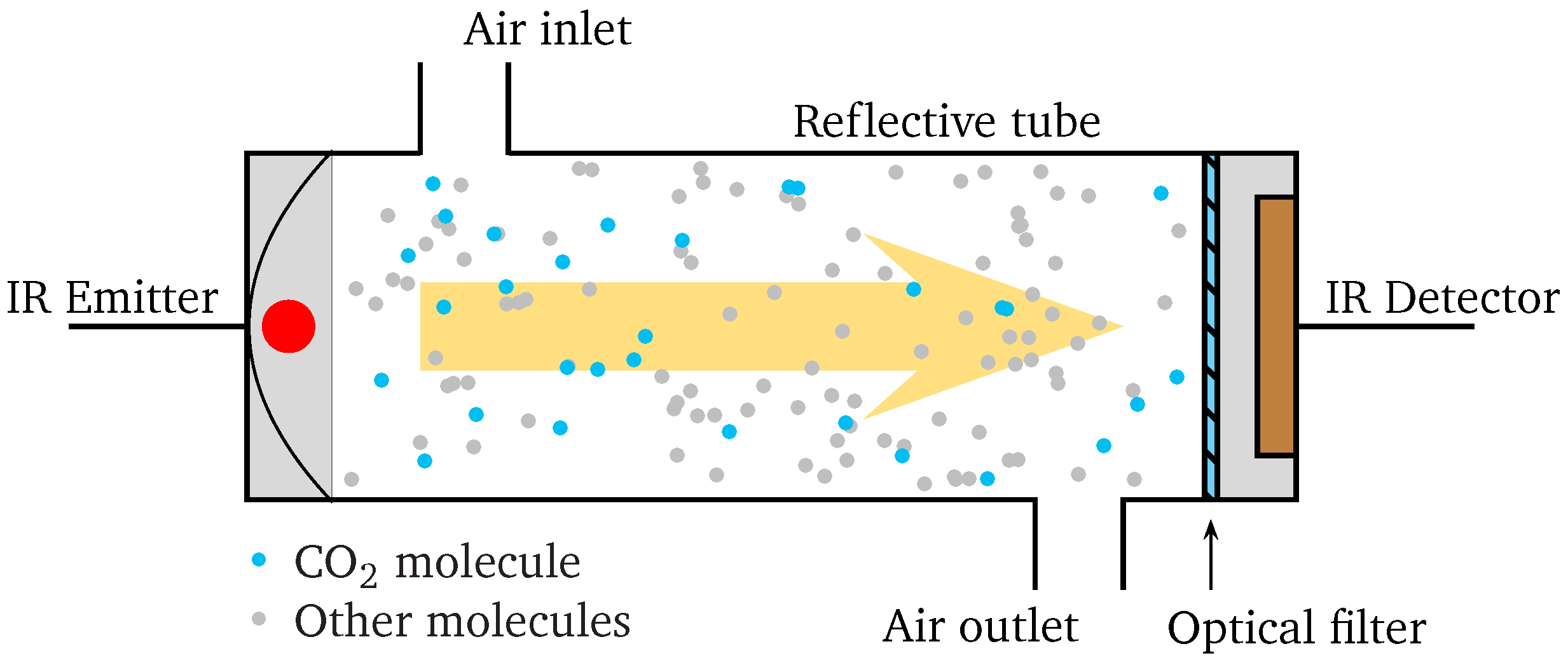
To measure the concentration of CO2 in the air, an NDIR sensor is used, which is quite precise and easy to calibrate. This sensor consists of a tube, an optical filter, an emitter, and an infrared (IR) detector, as shown in Figure 2. The emitter produces IR light waves that travel through the air sample tube. The IR waves move toward the optical filter in front of the detector. The detector measures the amount of IR light that passes through the filter.
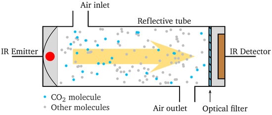
Figure 2.
CO2 sensor.
The radiation emitters band coincides with the CO2’s absorption band, located around 4.26 μm. The absorption spectrum is unique, so it is a signature or fingerprint to identify the CO2 molecule.
As IR light travels through the tube, the CO2 gas molecules absorb the characteristic 4.26 μm band while letting other wavelengths pass. At the detector end, the remaining light is incident on an optical filter that absorbs all wavelengths of light except the wavelength absorbed by the CO2 molecules in the tube containing the air sample.
Finally, the detector receives the remaining amount of IR light not absorbed by the CO2 molecules or the optical filter. To calculate the CO2 concentration, the difference between the amount of IR light radiated by the emitter and the amount of IR light received by the detector is measured. Since this difference results from light absorption by the CO2 molecules in the tube, it is directly proportional to the number of CO2 molecules in the air sample.
In the monitoring station where the sensor is embedded, some aspects are taken into account so that the measurements are as accurate as possible; one of them is the warm-up time, which lasts approximately 60 s; during this time, the data are unreliable and are not recorded. In addition, the sensor must be calibrated using a process that references the lowest concentration recorded outdoors over some time. To verify the proper operation and accuracy of each NDIR sensor, its readings are compared to those of a precision CO2 meter to validate the calibration.
The CO2 concentrations recorded by the sensor vary depending on where it is placed within the monitored space; for a reliable reading, considering the influence of ventilation, the sensors are placed at least 120 cm from the ground, 60 cm from air flows (windows), and SI2m of the people inside the room, as suggested by previous studies [17].
2.2. Monitoring Stations
The monitoring stations capture the measurements from the sensors to transmit them in an IoT network where the measurements of all the monitored classrooms or offices converge. Each station is made up of the following elements:
- An ESP32 microcontroller module with WiFi, Bluetooth, and LoRa wireless connections; it also allows wired connections using I2C, UART, and SPI protocols.
- An NDIR sensor model MH-Z19D with UART-type serial interface; its detection range goes from 400 ppm to 10,000 ppm, with a maximum error of 50 ppm.
- Connection to an IoT network by WiFi or LoRa (long-range radio frequency), depending on the wireless connectivity available in each station.
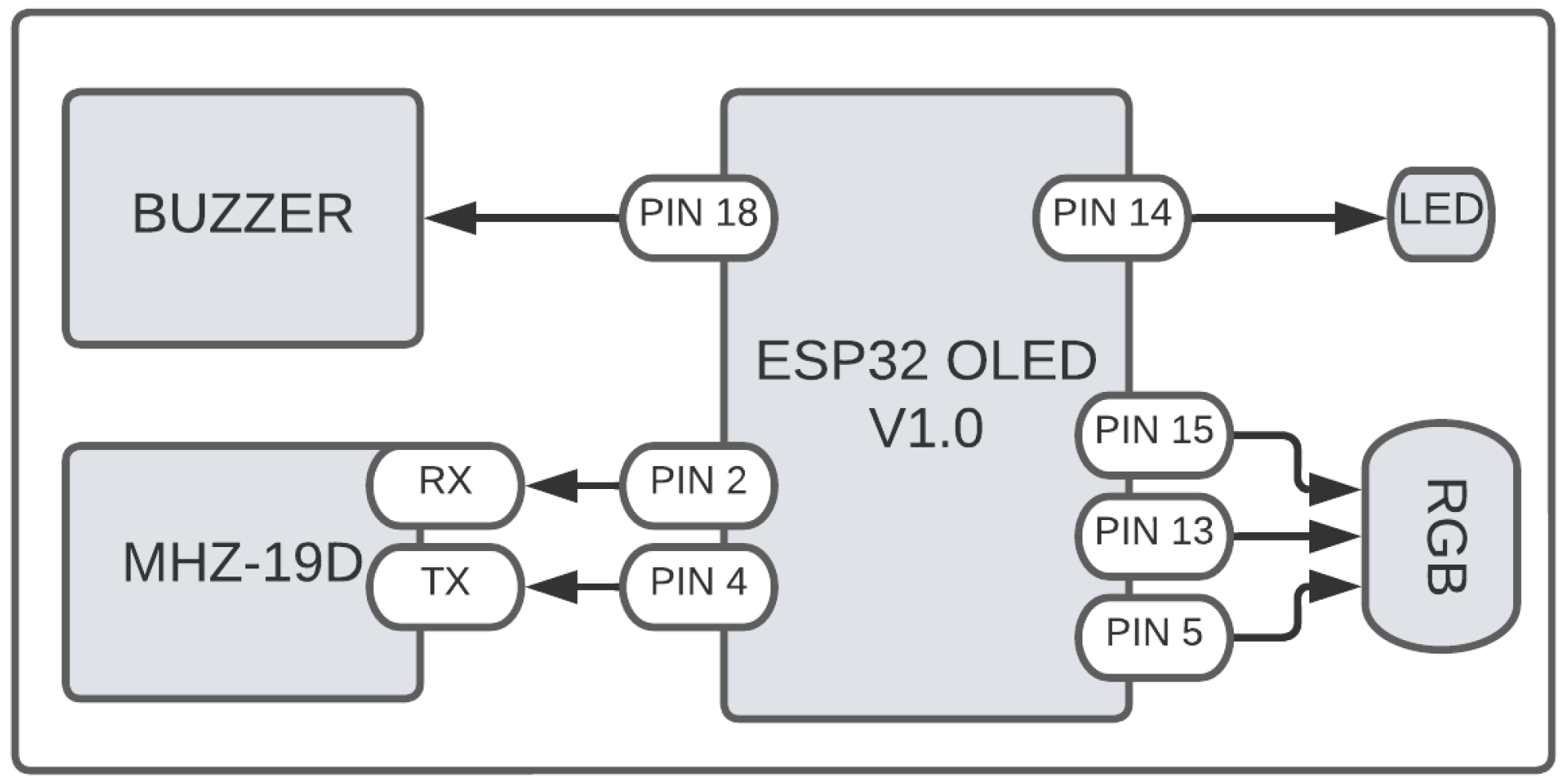
The microcontroller captures the values the NDIR sensor detects and sends the data wirelessly for recording and processing in the cloud. The electrical diagram of the M5 tough device is shown in Figure 3, where the connections of the microcontroller with the sensor and the visual/sound indicators used as an alarm are specified when the concentration of CO2 exceeds the safe values; and its specifications are presented in Table 2.
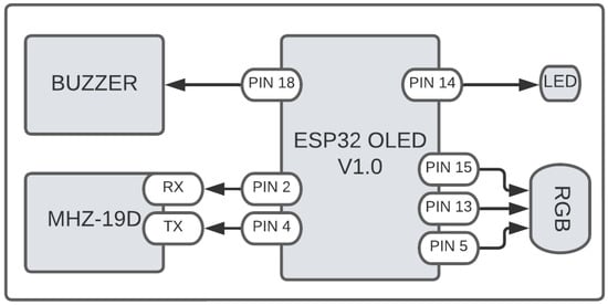
Figure 3.
Connections at the monitoring station.
Table 2.
Technical data for M5TOUGH.
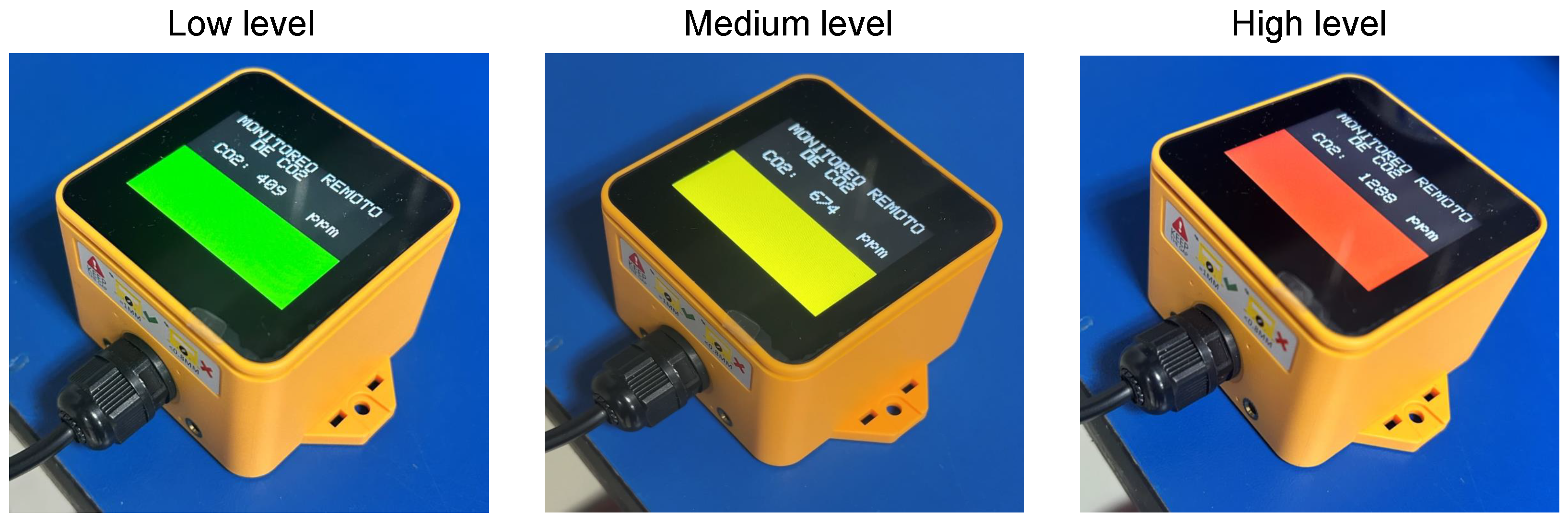
The monitoring stations comprise an IoT network managed by ThingSpeak, a Cloud Computing service operated by MathWorks. The data are stored in the cloud, which can be updated and viewed using the ThingSpeak API, allowing them to be viewed on computers or mobile devices connected to the internet. The final prototype is presented in Figure 4, where the three concentration levels of CO2 are shown, according to ppm and visual indicators (green, yellow, and red). The design includes a 2 cm hole which allows air to flow freely through it, thus facilitating readings from the CO2 sensor. The marked levels are presented according to Table 3.

Figure 4.
CO2 concentration levels with indicator colors.
Table 3.
Risk levels according to [18].
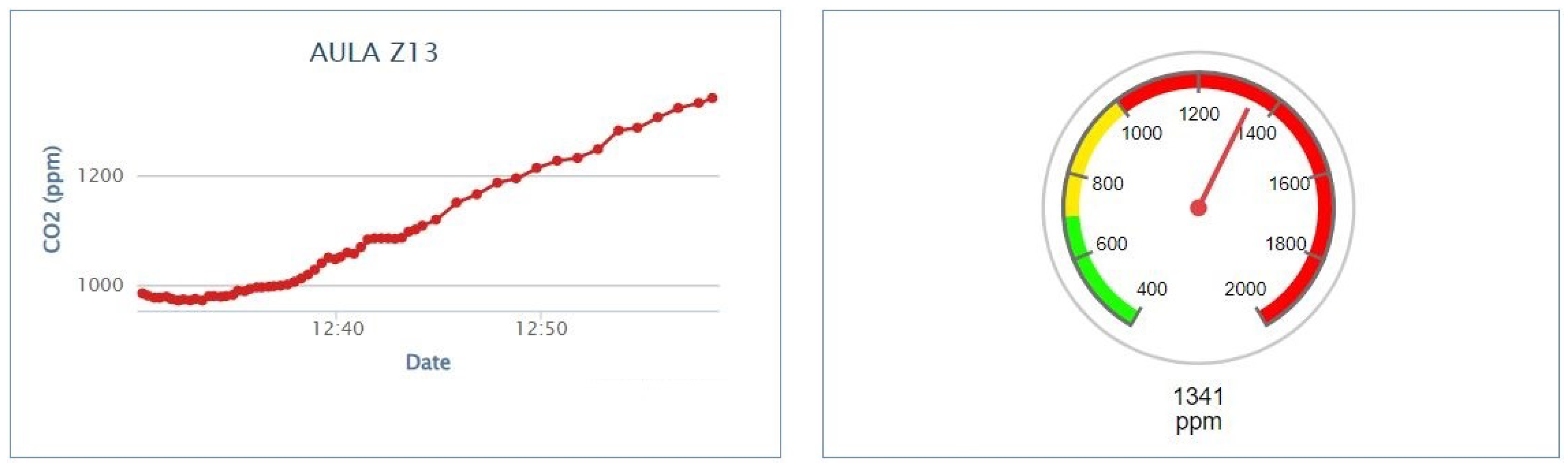
The screenshot in Figure 5 shows the remote interface of one of the stations. The sensor sampling period is one second, although the cloud data are updated every 15 s due to limitations in bandwidth and available storage space; the communication latency is approximately one second, which is sufficient considering the frequency of data updating and the slow dynamics in the monitored area since there are no sudden changes in the concentration of CO2.
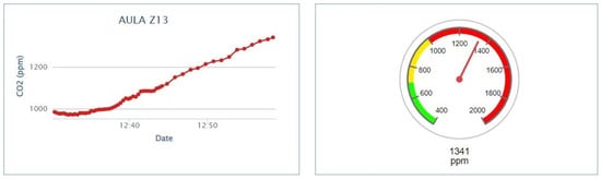
Figure 5.
Monitoring interface in ThingSpeak.
2.3. Prognosis of CO2 Concentration with LSTM Network
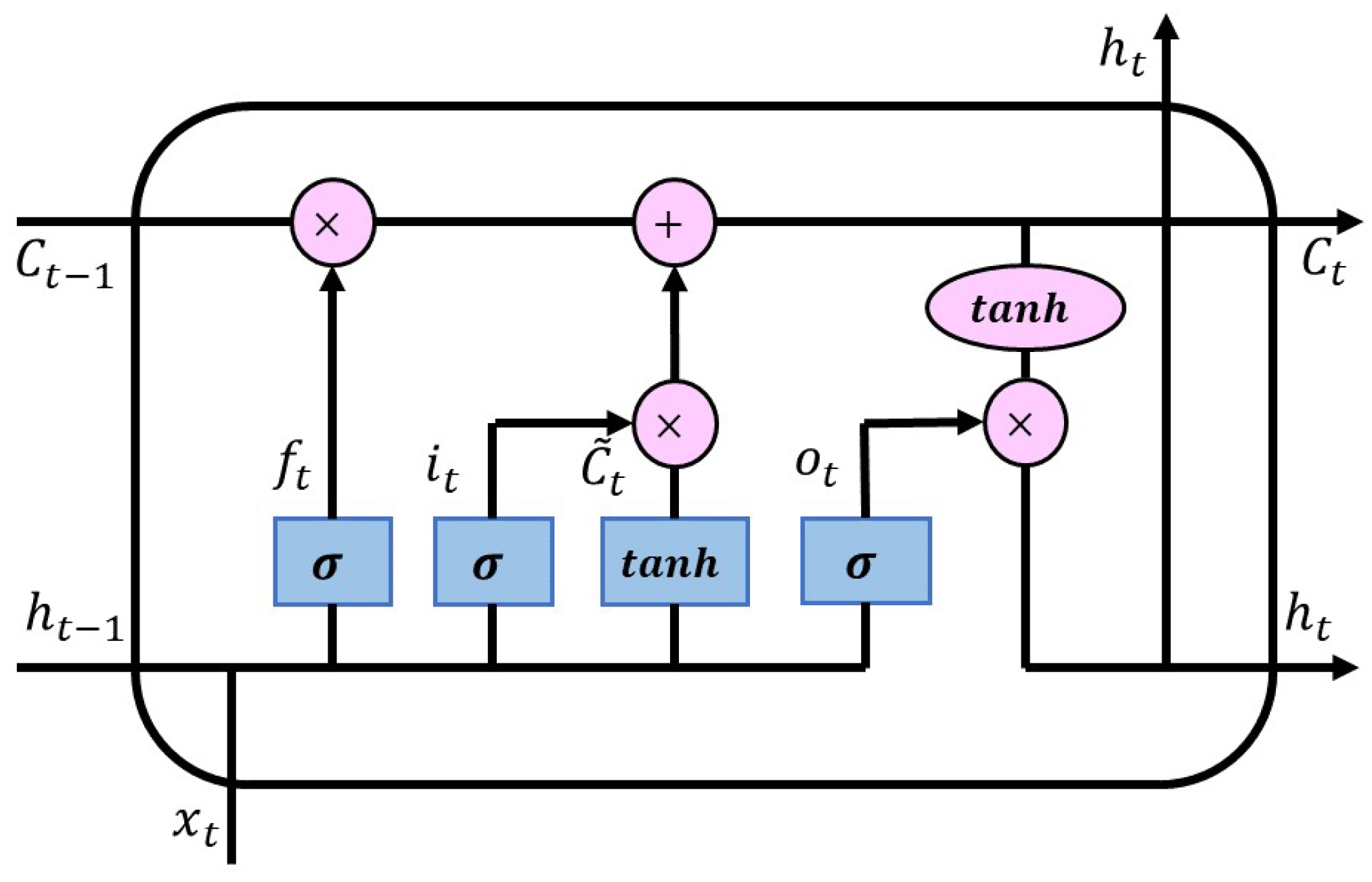
A type of neural network based on deep learning frequently used in time–series forecasting is autoregressive networks and those called Long Short-Term Memory (LSTM). From the CO2 concentrations recorded by the stations, time–series are created for each monitored classroom, which are used to estimate future CO2 concentrations based on the most recent measurements. LSTM networks work with time–series processing, using loops in their network diagram, and allowing them to remember/forget previous states and use this information to decide the next one. This LSTM comprises a status cell that transmits the data to be processed through the network. This gate allows us to decide what information is going to be discarded and another allows us to update the memory, as shown in Figure 6 and as expressed in Equations (1)–(6). Where are the input data; , , and , are the outputs of each gate, enabled by the activation function, or tanh. The subscripts f, i, and o are indicative of the gate that corresponds to them, forget, input, and output. In addition, there are short- and long-term memories, and .

Figure 6.
Structure of an LSTM network.
Conventional recursive networks are used to model short-term dependencies (i.e., close relationships in time–series), whereas LSTMs are useful for modeling long-term dependencies. The LSTM architecture is a block comprising three neural networks, better known as gates, which allow us to weigh the dataset to remember, discard, and update the information at the convenience of its application. This network will enable us to make a more extended prediction due to its long-term memory derived from the gates above. The LSTM block configurations are presented, which were proposed to analyze its performance with the dataset described above. The LSTM configurations were trained with 70% of the available data, and the other 30% were used to perform the forecast tests. The Adam learning algorithm was used with an initial learning rate of 0.005, and the iterations for the training were varied to know its impact on the performance of the network.
The number of hidden units and training times were varied in the neural architecture tuning. The first configuration selected took 200 epochs to train, having 128 hidden units. The second setup was 30 hidden units and trained in 1000 epochs. The third analysis case was of 208 hidden units and was trained in 1000 epochs.
3. Results and Discussion
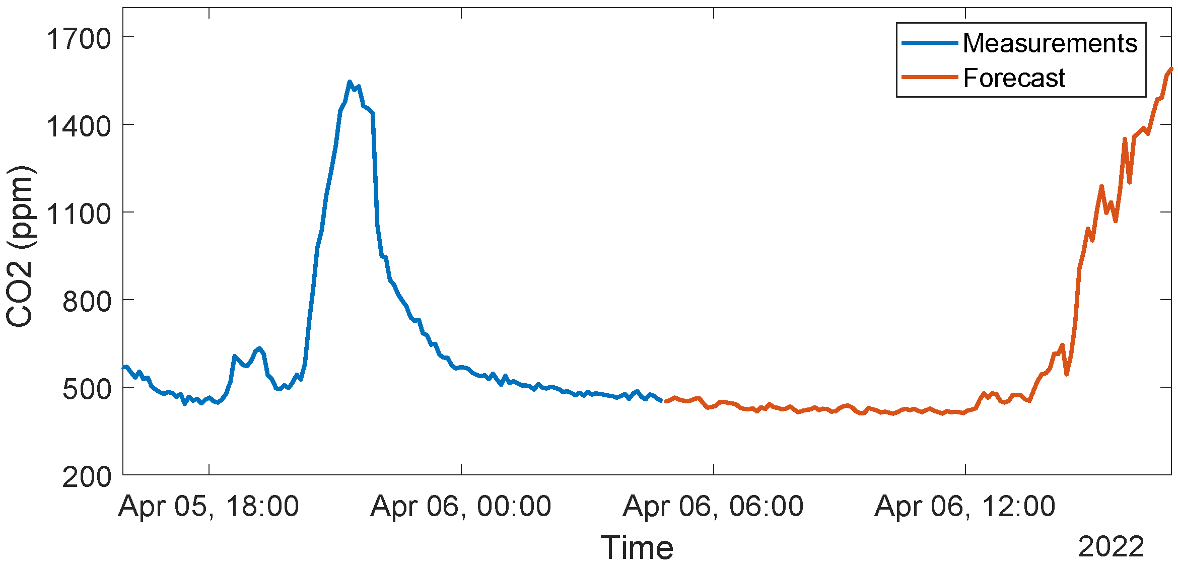
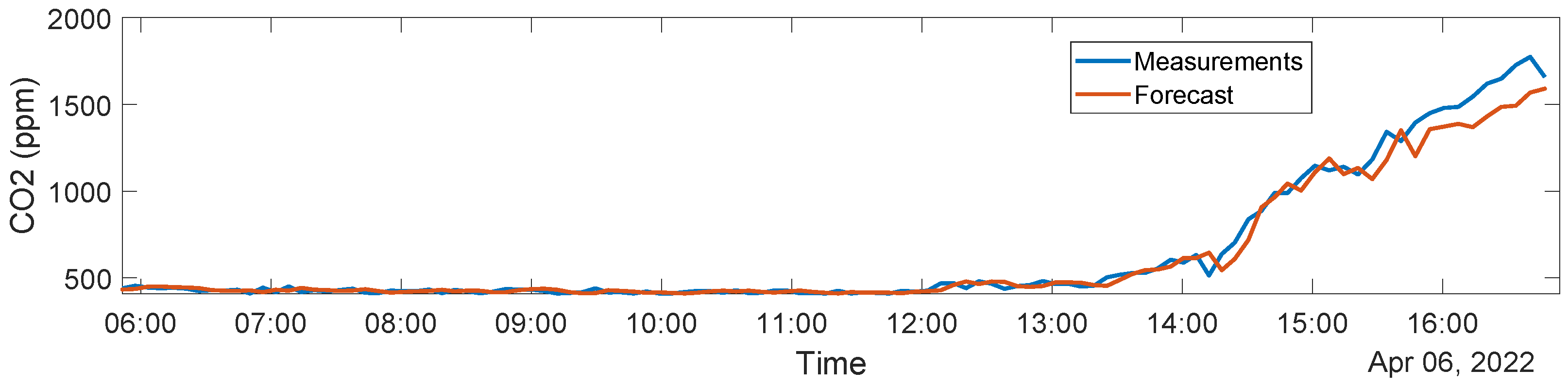
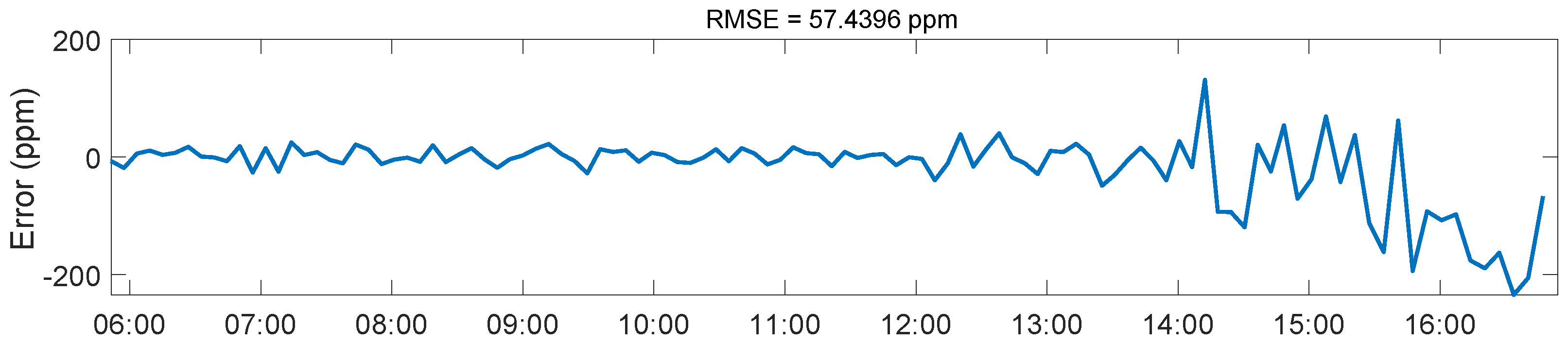
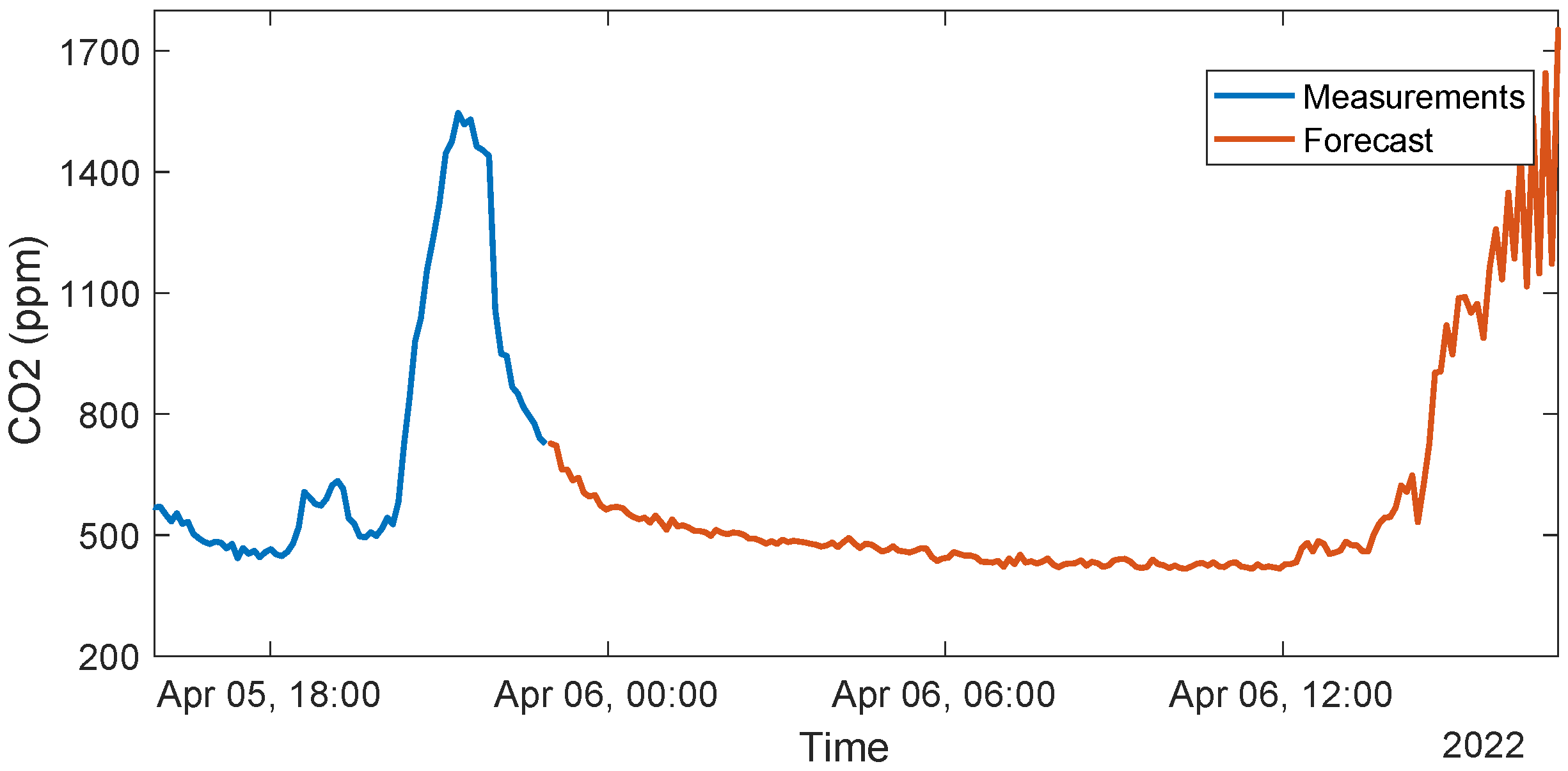
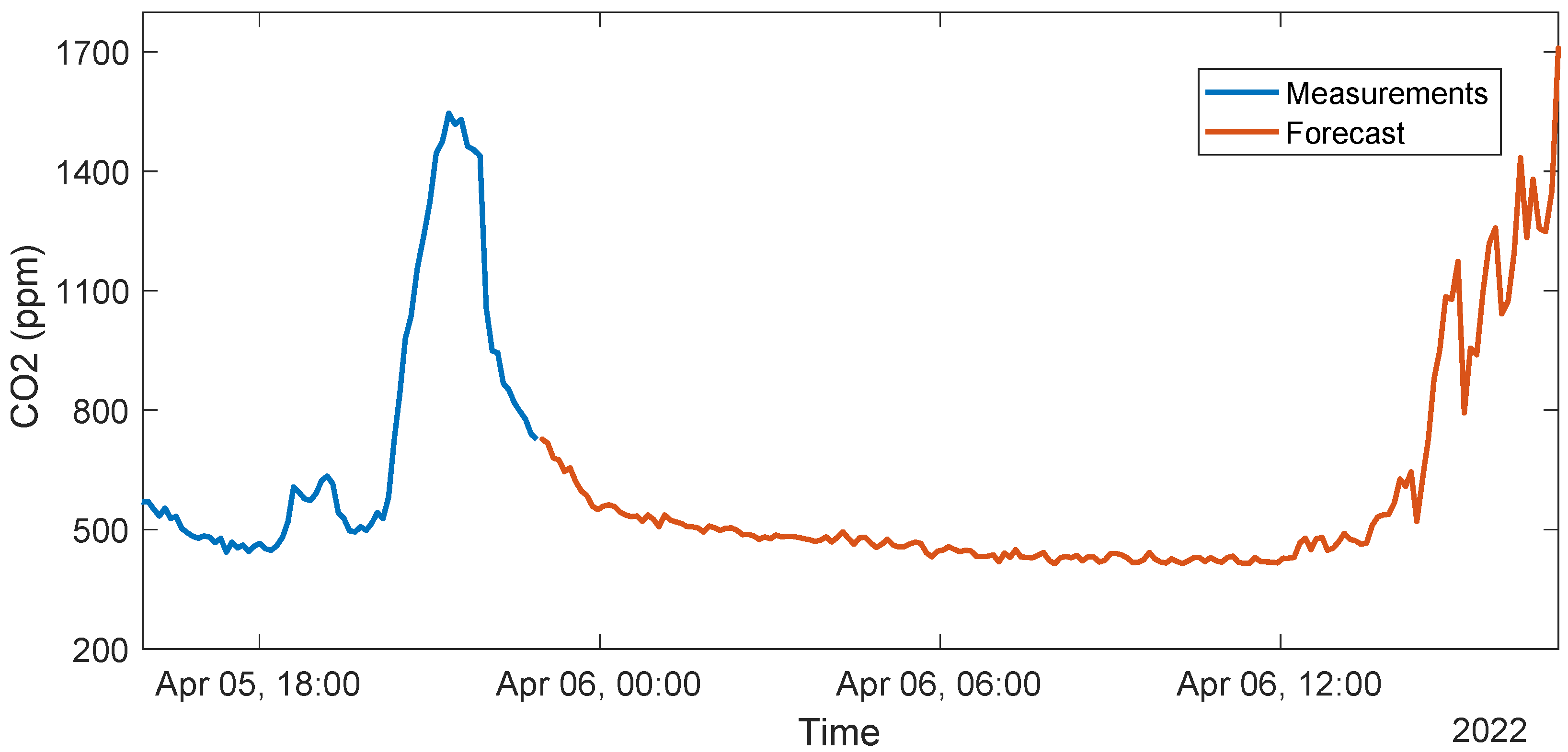
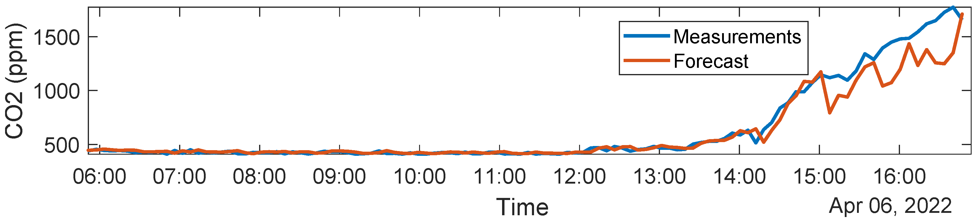
The previously mentioned configurations of the LSTM block, varying the number of hidden units (128, 30, and 208 units), registered the best performances, obtaining accurate forecasts with a competitive RMSE, being lower concerning the results obtained with the NAR architecture. The first configuration with 128 hidden units took 200 epochs to train, obtaining an RMSE of 57.4396 ppm, an MAD of 27.67 ppm, and an MAPE of 0.026887%. Figure 7 shows the network output, Figure 8 contrasts the measured and forecast data, whereas Figure 9 presents the error between them.

Figure 7.
Neural network output, Case 1 LSTM.
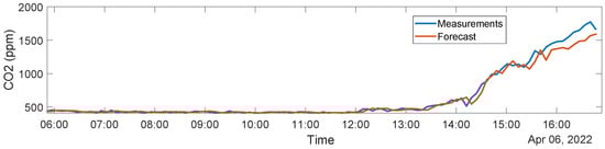
Figure 8.
Measured data versus predicted data, Case 1 LSTM.
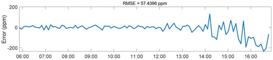
Figure 9.
Forecast error, Case 1 LSTM.
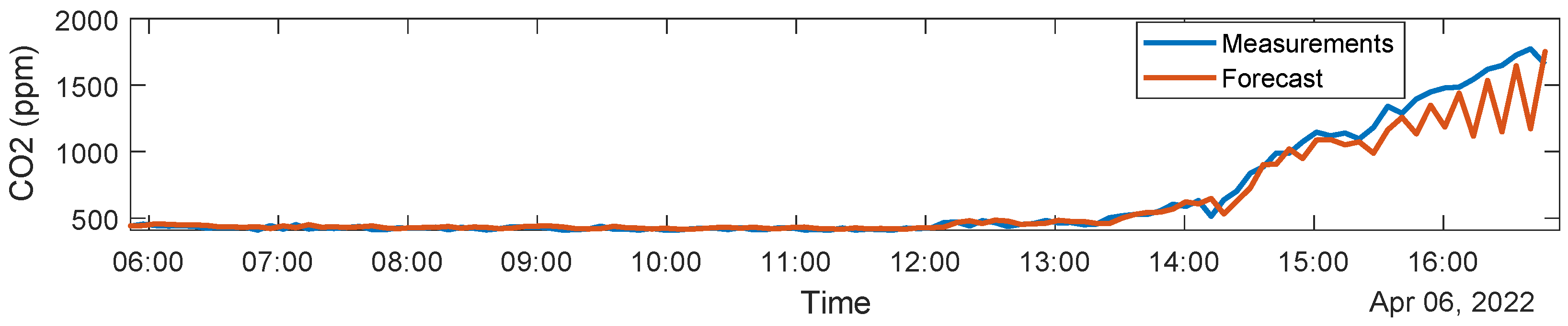
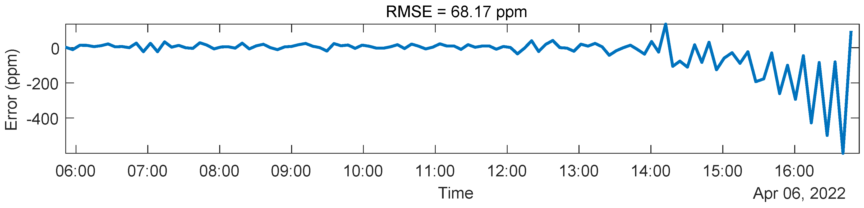
The second configuration with 30 hidden units took 1000 epochs to train, obtaining an RMSE of 68.17 ppm, an MAD of 31.33 ppm, and an MAPE of 0.02871%. Figure 10 shows the network output, Figure 11 contrasts the measured and forecast data, and Figure 12 presents the error between them.
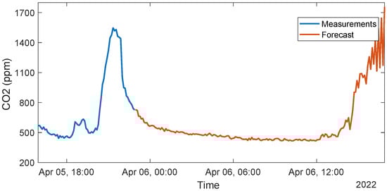
Figure 10.
Neural network output, Case 2 LSTM.
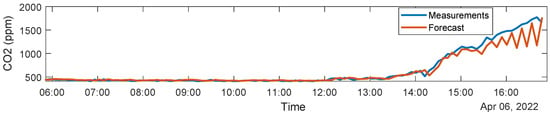
Figure 11.
Measured data versus predicted data, Case 2 LSTM.
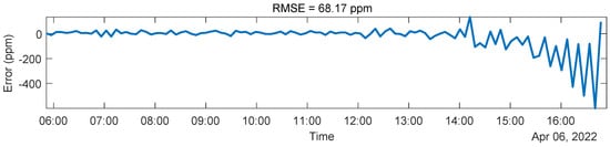
Figure 12.
Forecast error, Case 2 LSTM.
The third configuration, with 208 hidden units, took 1000 epochs to train, obtaining an RMSE of 69.86 ppm, an MAD of 29.1748 ppm, and an MAPE of 0.017992%. Figure 13 shows the network performance, Figure 14 contrasts the measured and forecast data, and Figure 15 presents the error between them.
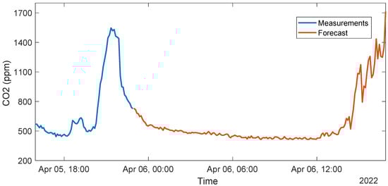
Figure 13.
Neural network output, Case 3 LSTM.
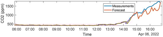
Figure 14.
Measured data versus predicted data, Case 3 LSTM.
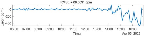
Figure 15.
Forecast error, Case 3 LSTM.
Validation of the Proposed LSTM
Different architecture configurations for the validation of the LSTM were analyzed, which are presented below (Table 4, Table 5, Table 6 and Table 7), highlighting the best performances. These tables are separated concerning selection percentages for training and test data to analyze their impact on configurations; in addition, they present the statistical indices to measure their performance. From this, it was concluded that the best results were obtained by selecting a data percentage of 70% for training and 30% for testing, maintaining the lowest RMSE on average.
Table 4.
LSTM validation: 80% training, 20% testing.
Table 5.
LSTM validation: 70% training, 30% testing.
Table 6.
LSTM validation: 60% training, 40% testing.
Table 7.
LSTM validation: second dataset.
In relation to the results obtained, a comparison is made with previous research carried out by other authors, who have addressed the analysis of the concentration of CO2 using various machine learning and deep learning approaches and techniques. These approaches and techniques are detailed in Table 8. A nonlinear autoregressive network (NAR) was tested, with a similar configuration presented for the LSMT of this work, the NAR obtained lower performance than the LSTM. On the other hand, the results were compared with the SVM, a linear regressive network (LR), and an artificial neural network (ANN) although its topology is not presented, reported in [19]. As can be seen, the proposed LSTM configuration obtained the lowest RMSE to predict CO2. Table 9 expands this comparison by summarizing the key differences between the study by Liu et al. and the present research; whereas Liu et al. [19] achieved lower RMSE values (16.77 ppm), their model is limited to a 1 min prediction window. In contrast, the proposed approach extends the forecast to 8 h, making it more suitable for long-term air quality management. Additionally, the methodology provides a detailed description of the IoT implementation, specifying the use of NDIR sensors and ESP32 microcontrollers, whereas Liu et al. do not specify their hardware components; while Liu et al. validated their study in a residential environment, the present research was tested in various indoor spaces, such as classrooms, offices, and laboratories, demonstrating broader applicability.
Table 8.
Summary of performances of different network architectures.
Table 9.
Comparison between Liu et al. [19] and the present study.
4. Conclusions
The implementation of an IoT-based LSTM model for CO2 monitoring has demonstrated high effectiveness in predicting CO2 levels up to 8 h in advance. The ability of LSTM networks to capture long-term dependencies in time–series data allows for accurate and reliable forecasting, surpassing the performance of NAR neural networks. The proposed system provides a scalable and cost-effective solution for real-time CO2 monitoring, offering valuable insights into air quality trends in shared indoor environments. These results highlight the potential of LSTM-based approaches to enhance air quality management by enabling proactive ventilation strategies and improving occupant well-being.
Future research could focus on optimizing the model’s hyperparameters to further enhance predictive accuracy. Additionally, integrating other environmental factors such as temperature, humidity, and air quality indices could refine the system’s performance. Developing a real-time alert mechanism for CO2 threshold exceedance would further improve its practical applicability, allowing for immediate corrective actions. Advancements in this area will contribute to the development of more intelligent and efficient air quality monitoring systems, fostering healthier and safer indoor environments.
Author Contributions
Conceptualization, M.J.M.-Z. and I.S.-R.; Data curation, E.-J.P.-P., A.N.-D. and J.-A.D.-A.; Formal analysis, A.N.-D., J.-A.D.-A. and E.-J.P.-P.; Methodology, M.J.M.-Z. and I.S.-R.; Project administration, I.S.-R.; Software, M.J.M.-Z. and E.-J.P.-P.; Supervision, I.S.-R.; Validation, M.J.M.-Z. and I.S.-R.; Visualization, E.-J.P.-P., A.N.-D. and J.-A.D.-A.; Writing—original draft, M.J.M.-Z., I.S.-R. and E.-J.P.-P.; Writing—review and editing, J.-A.D.-A. and A.N.-D. All authors have read and agreed to the published version of the manuscript.
Funding
This research has been supported by the Consejo Nacional de Humanidades, Ciencias y Tecnologías (CONAHCyT) and by Tecnológico Nacional de México (TecNM).
Data Availability Statement
The raw data supporting the conclusions of this article will be made available by the authors on request.
Conflicts of Interest
The authors declare no conflicts of interest.
References
- Moreno Grau, S.; Álvarez León, E.; García dos Santos Alves, S.; Diego Roza, C.; Ruiz de Adana, M.; Marín Rodríguez, I.; Rodríguez-Ba no, J.; Tomás Carmona, M.; Minguillón, M.C.; van der Haar, R. Evaluación del Riesgo de la Transmisión de SARS-CoV-2 Mediante Aerosoles. Medidas de Prevención y Recomendaciones. Documento Técnico. Ministerio de Sanidad. 2020. Available online: https://www.sanidad.gob.es/profesionales/saludPublica/ccayes/alertasActual/nCov/documentos/COVID19_Aerosoles.pdf (accessed on 30 December 2024).
- Lahrz, T.; Bischof, W.; Sagunski, H.; Baudisch, C.; Fromme, H.; Grams, H.; Gabrio, T.; Heinzow, B.; Müller, L. Gesundheitliche Bewertung von Kohlendioxid in der Innenraumluft. Bundesgesundheitsblatt Gesundheitsforschung Gesundheitsschutz 2008, 51, 1358–1369. [Google Scholar]
- Zemitis, J.; Bogdanovics, R.; Bogdanovica, S. The study of CO2 concentration in a classroom during the COVID-19 safety measures. E3S Web Conf. 2021, 246, 01004. [Google Scholar]
- Peng, Z.; Jimenez, J.L. Exhaled CO2 as a COVID-19 infection risk proxy for different indoor environments and activities. Environ. Sci. Technol. Lett. 2021, 8, 392–397. [Google Scholar] [PubMed]
- Minguillón, M.; Querol, X.; Riediker, M.; Felisi, J.; Garrido, T.; Alastuey, A.; Bekö, G.; Nehr, S.; Wiesen, P.; Carslaw, N. Guide for Ventilation Towards Healthy Classrooms. COST (European Cooperation in Science and Technology) Action CA17136 Report. 2020. Available online: https://scoeh.ch/wp-content/uploads/2021/01/Guide-for-ventilation_Indairpollnet.pdf (accessed on 30 December 2024).
- Martin, C.R.; Zeng, N.; Karion, A.; Dickerson, R.R.; Ren, X.; Turpie, B.N.; Weber, K.J. Evaluation and environmental correction of ambient CO2 measurements from a low-cost NDIR sensor. Atmos. Meas. Tech. 2017, 10, 2383–2395. [Google Scholar]
- Tripathi, B.S.; Gupta, R.; Reddy, S. Cloud Architecture Based Learning Kit Platform for Education and Research—A Survey and Implementation. In Proceedings of the International Symposium on Ubiquitous Networking, Virtual, 19–21 May 2021; pp. 172–185. [Google Scholar]
- Robin, Y.; Amann, J.; Baur, T.; Goodarzi, P.; Schultealbert, C.; Schneider, T.; Schütze, A. High-performance VOC quantification for IAQ monitoring using advanced sensor systems and deep learning. Atmosphere 2021, 12, 1487. [Google Scholar] [CrossRef]
- Altikat, S.; Gulbe, A.; Kucukerdem, H.K.; Altikat, A. Applications of artificial neural networks and hybrid models for predicting CO2 flux from soil to atmosphere. Int. J. Environ. Sci. Technol. 2020, 17, 4719–4732. [Google Scholar]
- Kapoor, N.R.; Kumar, A.; Kumar, A.; Kumar, A.; Mohammed, M.A.; Kumar, K.; Kadry, S.; Lim, S. Machine Learning-Based CO2 Prediction for Office Room: A Pilot Study. Wirel. Commun. Mob. Comput. 2022, 2022. [Google Scholar] [CrossRef]
- Kwon, J.; Ahn, G.; Kim, G.; Kim, J.C.; Kim, H. A study on NDIR-based CO2 sensor to apply remote air quality monitoring system. In Proceedings of the 2009 ICCAS-SICE, Fukuoka, Japan, 18–21 August 2009; pp. 1683–1687. [Google Scholar]
- Marques, G.; Pitarma, R. Monitoring health factors in indoor living environments using internet of things. In Recent Advances in Information Systems and Technologies; Springer: Cham, Switzerland, 2017; Volume 570, pp. 785–794. [Google Scholar]
- Marques, G.; Ferreira, C.R.; Pitarma, R. Indoor air quality assessment using a CO2 monitoring system based on internet of things. J. Med. Syst. 2019, 43, 67. [Google Scholar] [CrossRef] [PubMed]
- Kallio, J.; Tervonen, J.; Räsänen, P.; Mäkynen, R.; Koivusaari, J.; Peltola, J. Forecasting office indoor CO2 concentration using machine learning with a one-year dataset. Build. Environ. 2021, 187, 107409. [Google Scholar]
- Arsiwala, A.; Elghaish, F.; Zoher, M. Digital twin with machine learning for predictive monitoring of CO2 equivalent from existing buildings. Energy Build. 2023, 284, 112851. [Google Scholar]
- Alsamrai, O.; Redel-Macias, M.D.; Pinzi, S.; Dorado, M. A systematic review for indoor and outdoor air pollution monitoring systems based on Internet of Things. Sustainability 2024, 16, 4353. [Google Scholar] [CrossRef]
- Nusseck, M.; Richter, B.; Holtmeier, L.; Skala, D.; Spahn, C. CO2 measurements in instrumental and vocal closed room settings as a risk reducing measure for a Coronavirus infection. medRxiv 2020. [Google Scholar] [CrossRef]
- Mesa Silva, A.F. Evaluación de los Niveles de Riesgo Ocupacional Asociado a las Concentraciones de Gases Contaminantes en Atmosferas Confinadas en un Acueducto. Available online: https://ciencia.lasalle.edu.co/items/34b05257-d236-46f5-89ca-7c59d583c2d2 (accessed on 30 December 2024).
- Liu, Z.; Ciais, P.; Deng, Z.; Lei, R.; Davis, S.J.; Feng, S.; Zheng, B.; Cui, D.; Dou, X.; Zhu, B.; et al. Near-real-time monitoring of global CO2 emissions reveals the effects of the COVID-19 pandemic. Nat. Commun. 2020, 11, 5172. [Google Scholar] [CrossRef] [PubMed]

Disclaimer/Publisher’s Note: The statements, opinions and data contained in all publications are solely those of the individual author(s) and contributor(s) and not of MDPI and/or the editor(s). MDPI and/or the editor(s) disclaim responsibility for any injury to people or property resulting from any ideas, methods, instructions or products referred to in the content. |
© 2025 by the authors. Licensee MDPI, Basel, Switzerland. This article is an open access article distributed under the terms and conditions of the Creative Commons Attribution (CC BY) license (https://creativecommons.org/licenses/by/4.0/).