Inducing Perceptual Dominance with Binocular Rivalry in a Virtual Reality Head-Mounted Display

Abstract

Binocular rivalry is the perceptual dominance of one visual stimulus over another. Conventionally, binocular rivalry is induced using a mirror-stereoscope—a setup involving mirrors oriented at an angle to a display. The respective mirror planes fuse competing visual stimuli in the observer’s visual field by projecting the stimuli through the stereoscope to the observed visual field. Since virtual-reality head-mounted displays fuse dichoptic vision in a similar way, and since virtual-reality head-mounted displays are more versatile and more readily available than mirror stereoscopes, this study investigated the efficacy of using a virtual-reality headset (Oculus Rift-S) as an alternative to using a mirror stereoscope to study binocular rivalry. To evaluate the validity of using virtual-reality headsets to induce visual dominance/suppression, two identical experimental sequences—one using a conventional mirror stereoscope and one using a virtual-reality headset—were compared and evaluated. The study used Gabor patches at different orientations to induce binocular rivalry and to evaluate the efficacy of the two experiments. Participants were asked to record all instances of perceptual dominance (complete suppression) and non-dominance (incomplete suppression). Independent sample t-tests confirmed that binocular rivalry with stable vergence was successfully induced for the mirror-stereoscope experiment (t = −4.86; p ≤ 0.0001) and the virtual-reality experiment (t = −9.41; p ≤ 0.0001). Using ANOVA to compare Gabor patch pairs of gratings at +45°/−45° orientations presented in both visual fields, gratings at 0°/90° orientations presented in both visual fields, and mixed gratings (i.e., unconventional grating pairs) presented in both visual fields, the performance of the two experiments was evaluated by comparing observation duration in seconds (F = 0.12; p = 0.91) and the alternation rate per trial (F = 8.1; p = 0.0005). The differences between the stimulus groups were not statistically significant for the observation duration but were significantly different based on the alternation rates per trial. Moreover, ANOVA also showed that the dominance durations (F = 114.1; p < 0.0001) and the alternation rates (F = 91.6; p < 0.0001) per trial were significantly different between the mirror-stereoscope and the virtual-reality experiments, with the virtual-reality experiment showing an increase in alternation rate and a decrease in observation duration. The study was able to show that a virtual-reality head-mounted display can be used as an effective and novel alternative to induce binocular rivalry, but there were some differences in visual bi-stability between the two methods. This paper discusses the experimental measures taken to minimise piecemeal rivalry and to evaluate perceptual dominance between the two experimental designs.

1. Introduction

Binocular rivalry (BR) occurs when competing stimuli are presented simultaneously to the respective visual fields, and one stimulus is unconsciously suppressed, whereas the other stimulus is consciously perceived [1,2,3,4,5,6,7,8]. Following the initial research on binocular rivalry [9,10], in 1996, Logothetis et al. proposed two separate forms of suppression that occur during binocular rivalry: eye suppression and stimulus suppression [11,12]. Further research was able to show that a visual field is suppressed during binocular rivalry, not a stimulus [11,13].Because the suppression occurs in the visual cortex, visual consciousness is often studied through BR [14,15,16]. BR can be demonstrated by a continuous pattern of alternating perceptual dominance (Figure 1), i.e., one of the two stimuli dominates for a certain period, while the other stimulus remains suppressed, followed by a continuous shift in dominance/suppression [16,17].

BR is subsequently measured by monitoring the alternation rate, overall predominance, and dominance duration for the respective dominance periods [18]. However, sometimes incomplete suppression can occur. This is referred to as piecemeal rivalry, (Figure 2), a phenomenon in which small parts of the suppressed stimulus still dominate and overlay the dominant percept [15]. Certain experimental measures can be taken to avoid piecemeal rivalry and ensure complete suppression. To study BR, it is important to avoid piecemeal rivalry by establishing and maintaining stable vergence [16]. Stable vergence can be achieved using fusion cues. Practically, fusion cues are often implemented by surrounding the rivalrous image pairs with identical frames—such as a simple patterned border—or by adding fixation crosses to the centre of the images [15]. Other factors that influence dominance during a BR task include contrast, spatial frequency, and brightness [18], which relate to the size and colour scale of the presented stimuli, as well as the refresh rate of the display. Images presented during BR tasks need to be emotionally neutral, have a simple semantic meaning, be identical in size (larger images evoke stronger occipital-lobe visually evoked potentials (VEPs) [19]), and have identical pixel contrasts and luminance [20].

Conventionally, Gabor patches are often used in BR [3] to ensure that all stimuli share certain low-level physical characteristics such as luminance, contrast, and spatial frequency. Gabor patches consist of suprathreshold sinusoidal gratings that are vignetted by a Gaussian envelope [21,22]. Gabor patches presented in rivalrous image pairs, with simple line gratings that share the same low-level characteristics, can have gratings of varying orientations to facilitate visual rivalry (Figure 3). Conventionally, studies consider Gabor patches in pairs of gratings with +45°/−45° orientations or 0°/90° orientations presented together [3,9]. The current study considered pairings of all four stimuli presented in Figure 3 to investigate the effects of different stimulus pairs on alternation rate and observation duration.

In cognitive neuroscience, BR is used to investigate when conscious experience manifests during visual processing, how and why visual selection happens during perceptual dominance, and to what extent the suppressed stimulus is being processed unconsciously [16]. Gabor patches have been accorded to early linear spatial filtering in the visual system [21] and have therefore been used to study BR. Research suggests that natural-image statistics evoke local interactions in early, feature-specific levels in the visual cortex [22].

A mirror stereoscope is an inexpensive way to induce and study BR [16]. Figure 4 shows a conventional BR setup using a stereoscope with a visual divider and several mirror planes. The respective mirror planes fuse competing visual stimuli in the observer’s visual field by projecting the stimuli through the stereoscope. Since virtual-reality (VR) head-mounted displays fuse dichoptic vision in a similar way to the planes in a mirror stereoscope, this study investigated the efficacy of using a virtual-reality headset (Oculus Rift-S) as an alternative method to study binocular rivalry. VR head-mounted displays are more versatile and more readily available than conventional mirror stereoscopes. There has also been a recent shift in cognitive research, where VR headsets have been used in several psychological experiments [24]. Using the alternative setup proposed in this research would benefit the field of BR research. The study therefore aimed to show that VR can be used as a reliable alternative to induce BR and to study its neurological effects.

2. Materials and Methods

All participants were required to complete a standard BR task twice: once while using a mirror stereoscope set up in front of a computer monitor, and once while wearing a VR headset (Section 2.2). The order in which participants completed the experiments was randomised, i.e., 16 participants completed the VR experiment first and 16 participants completed the mirror-stereoscope experiment first. Having the order of the tasks randomised also eliminated observational biases during one experiment compared to the other as a result of fatigue. The standard BR task was repeated to compare the performance of the conventional mirror stereoscope to the performance of the VR headset when inducing BR.

Thirty-two participants between the ages of 23 and 61 (the mean age was 32.4 years; SD = 9.34) volunteered to take part in the study (20 male; 12 female). Figure 5 shows the demographic distribution of the sample). The research did not distinguish between participants based on age or sex for analysis. All participants were required to have normal or corrected-to-normal vision. Individuals with corrected vision were permitted to take part only if they wore contact lenses. Participants wearing spectacles were excluded from consideration since the lenses can interfere with the effects of BR [19]. All participants provided written informed consent prior to taking part in the study, and the research experiment was approved by Stellenbosch University’s Health Research and Ethics Committee (HREC; reference number: S20/11/332). The study was conducted in accordance with the ethical guidelines and principles of the international Declaration of Helsinki, the South African Guidelines for Good Clinical Practice, and the Medical Research Council (MRC) Ethical Guidelines for Research.

2.1. Materials

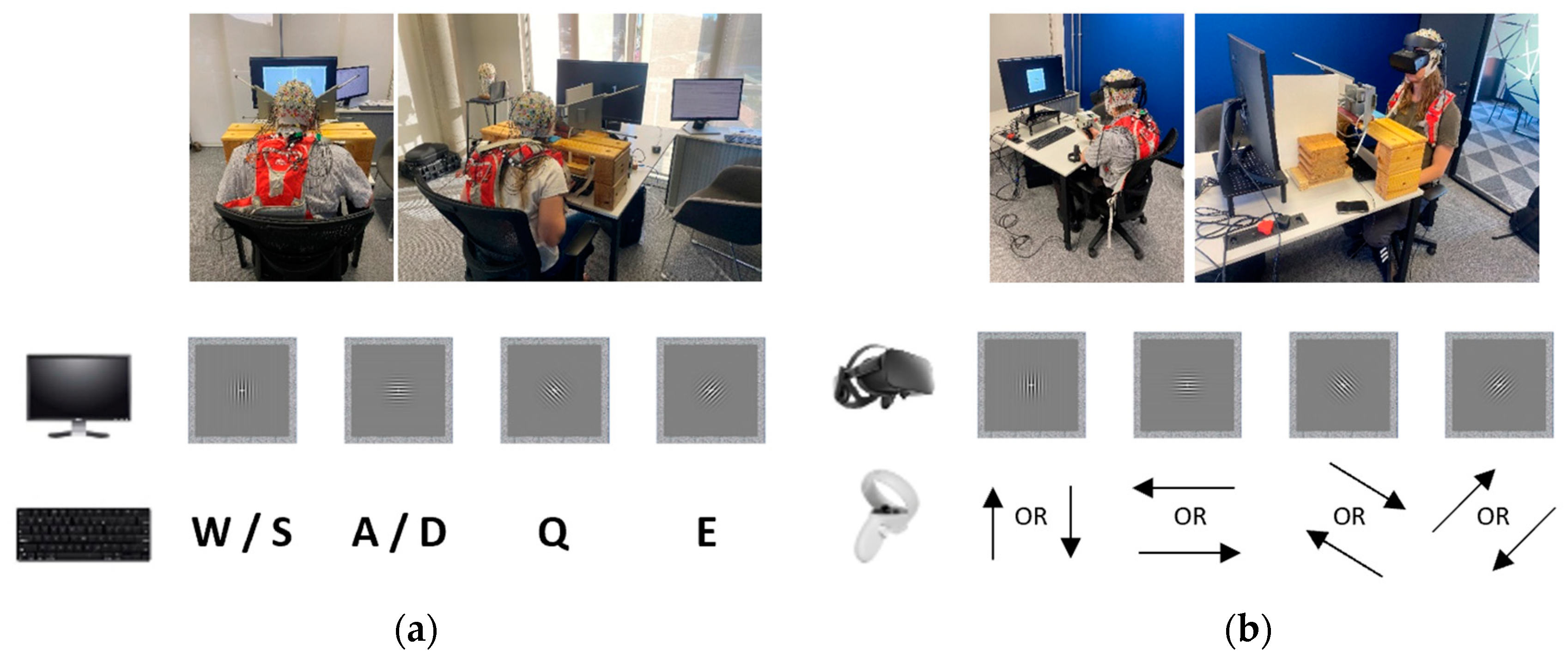
2.1.1. Mirror Stereoscope and VR Headset

The BR tasks were scripted using Unreal Engine [25], a standard software package used for creating virtual environments for VR headsets. Unreal Engine [25] was used for both the conventional (mirror stereoscope) and novel (VR headset) experimental paradigms. Figure 6 demonstrates how participants interacted with the mirror stereoscope (Figure 6a) and the VR headset (Figure 6b). When completing the mirror-stereoscope task, participants rested their heads on a wooden structure while looking through the viewports on the stereoscope. As shown in Figure 4, the stereoscope projected the stimuli, separated on a split computer screen (one stimulus presented on the left; one stimulus presented on the right), to the respective visual fields [26]. The computer screen, shown in Figure 6, was a 21” Dell monitor with a refresh rate of 60 Hz and a resolution of 1024 × 768 pixels. The VR headset, also shown in Figure 6, was an Oculus Rift-S headset with a refresh rate ranging from 40 to 60 Hz and a resolution of 1280 × 800 (640 × 800 per eye). The interpupillary distance (IPD) was fixed at the headset’s default of 63.5 mm, whereas the fixed focal distance for the headset was at 1.3 m. The headset’s apparent distance to the stimulus was manipulated by setting the y-axis coordinate to 200 mm—this change was made to establish stable vergence in the VR headset (see Appendix A). The visual tasks were completed in a dimly lit, quiet room.

When interacting with the mirror stereoscope, participants recorded their responses by pressing and releasing a specific key using a standard keyboard. When interacting with the VR headset, participants recorded their responses using the VR headset’s right-hand controller by pressing and releasing the thumb stick in the desired direction. Figure 6 shows how these responses were mapped to the orientation of the gratings of the Gabor patches. For the mirror stereoscope, the keys were mapped to the direction of the gratings of the Gabor patches by using standard gaming keys for movement in a virtual space (up/down = W/S; left/right = A/D; left diagonal = Q; right diagonal = E). For the VR headset, the Cartesian coordinates of the right controller’s thumb stick were mapped to the direction of the gratings of the Gabor patches. Participants could choose to use either the up or the down direction on the thumb stick that matched the orientation of the respective gratings. In cases of piecemeal rivalry, participants responded with the space bar on the keyboard and the trigger on the right controller for the respective experiments. The sensitivity of the controller was tested and adjusted.

For the mirror-stereoscope task, the height of the chair and the mirror structure was adjusted until participants reported that image fusion and BR occurred easily. For the VR headset, the tightness and placement of the headset was adjusted until participants reported seeing only one stimulus and clear instances of BR. Interpupillary distances were not adjusted between participants. Instead, the measure of the ease and clarity at which fusion and BR occurred relied on subjective reports by participants. Once the setup was reportedly working properly, the BR tasks started. For each experiment, participants performed a few tests to make sure they understood the task before the task started being recorded.

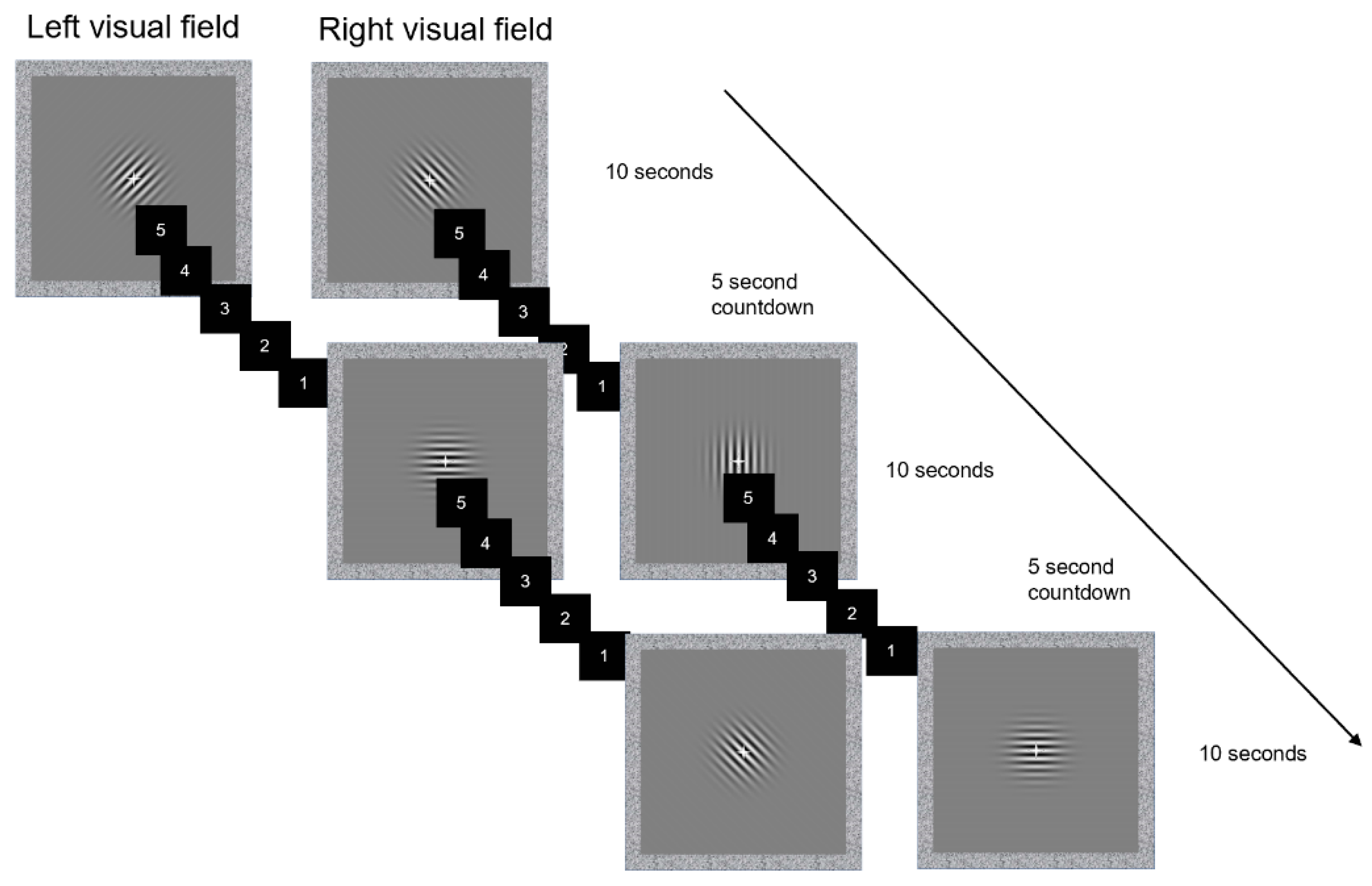
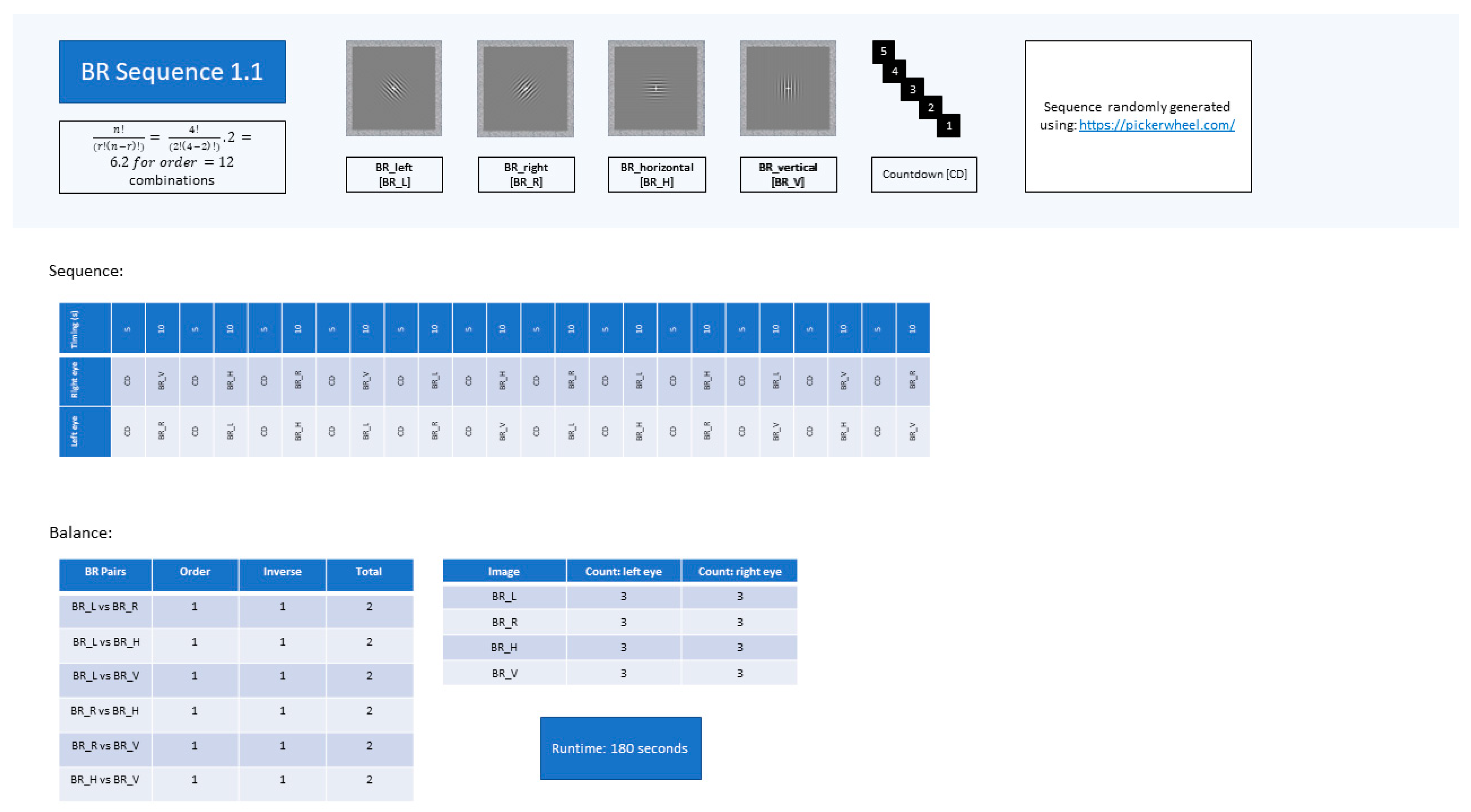
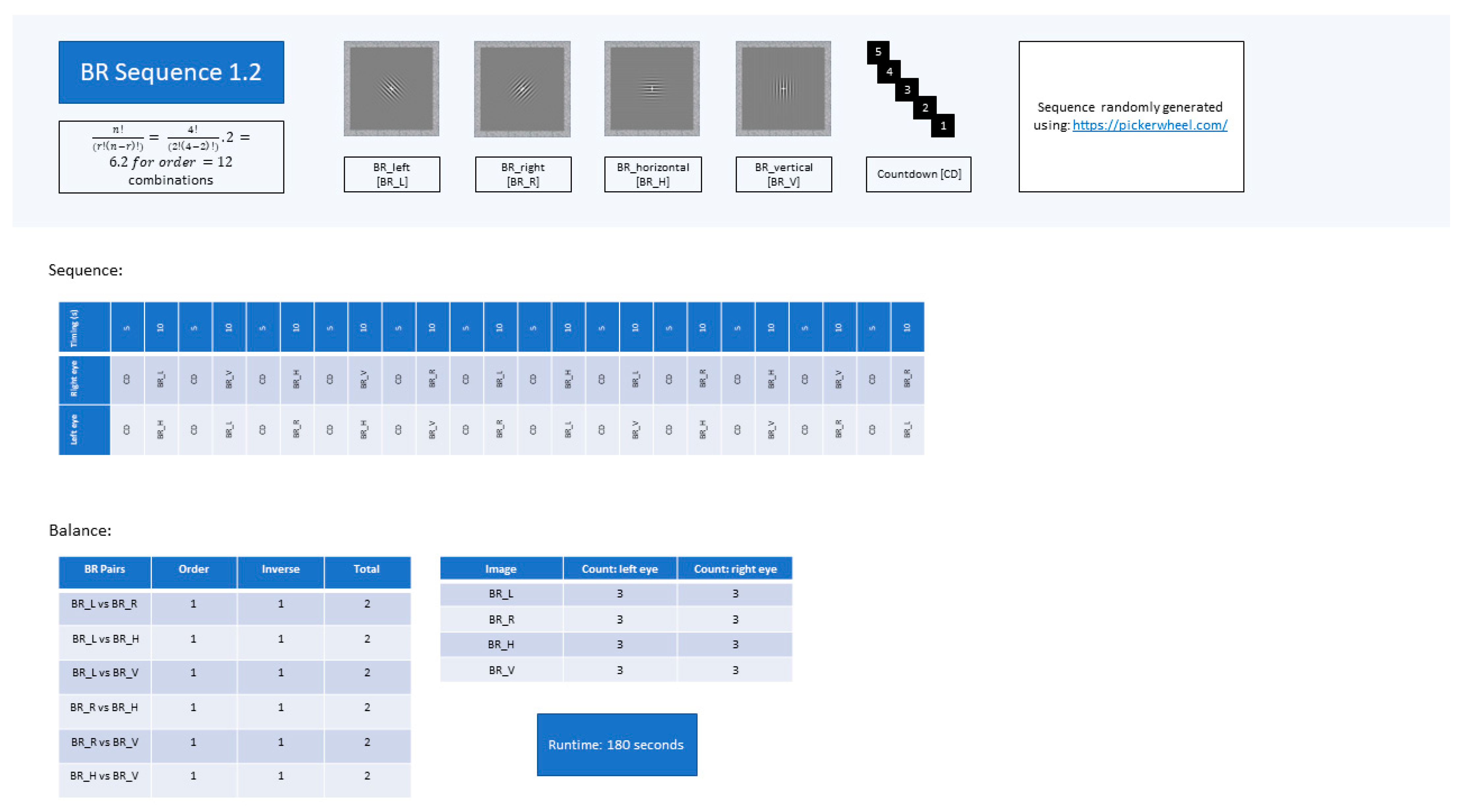
2.1.2. Visual Stimuli

For the visual stimuli, Gabor patches with four different grating orientations—with matching luminance, contrast, and spatial frequencies—were used (Figure 3) [26]. The rival Gabor patches shared the following characteristics: a Gaussian envelope with a standard deviation of σ = 20 pixels displayed at 100% contrast, a zero-phase spatial frequency of 1.15, a background colour of 124.75 cd/m², and two contrasting colours of 254.57 cd/m² and 0 cd/m². The only distinction between the four stimuli was the orientation of their gratings (horizontal (degrees = 0°), vertical (degrees = 90°), left diagonal (degrees = −45°), right diagonal (degrees = 45°)) [23]. The stimuli used during the experiments can be seen in Figure 3.

In experimental trials preceding the BR experiments, different iterations of stimuli and fusion cues were tested to establish and evaluate stable vergence (Appendix A). Appendix A summarises the improvements made to the stimuli. The rate of success was measured by comparing observations of stable vergence (perceptual dominance) to observations of piecemeal rivalry (non-dominance). Stable vergence ensures that the rivalrous images fall on corresponding locations of the respective retinae [15]. The mirror stereoscope worked well to induce BR in all cases, but stable vergence needed to be improved for the VR headset (Appendix A). To improve stable vergence in the VR headset, adjustments were made to the distance to the field (i.e., the y-axis distance in the VR headset), the refresh rate of the display, and the presence and style of the fusion cues.

To establish and maintain stable vergence, stimuli can be surrounded by the same frame, as well as by placing an identical fixation point at the centre of each image [15]. The distance to the visual field (the distance between the mirror stereoscope and the screen; and the y-axis distance in the VR headset), the refresh rate of the display, the presence or absence of fusion cues, and the colours of the stimuli all affect how successfully stable vergence can be achieved, and therefore how successfully BR can be induced. The refresh rate of the display—specifically, the discrepancy between the refresh rate of an external display and a VR headset—notably influences the efficacy of establishing and maintaining stable vergence.

No changes were made to the colours of the stimuli because the Gabor patches had alternating black and white gratings with matching contrasts. Colour was therefore not used as a variable to improve BR.

2.2. Method

For both experimental tasks, participants followed the sequence shown in Figure 7. Twelve different competing stimulus pairs were presented during each experimental sequence. A sequence of rivalrous pairs consisted of six novel combinations of the four distinct stimuli presented to the observer’s respective visual fields (calculated using the combinatoric formula). The different novel pairings were repeated, swapping around the left-/right-visual-field positions of the stimuli to ensure that the order of presentation was counterbalanced to eliminate visual-field dominance as cause for perceptual bias during BR [27]. This resulted in a sequence of 12 pairings. Two unique sequences, BR1.1 and BR1.2, of 12 rivalrous pairs per sequence, were scripted (see Appendix B). Each sequence contained the same stimulus pairings in varying chronologies. Both sequences were equally balanced to avoid perceptual bias and excessive observational repetition (see Appendix B).

For all participants, each sequence was either paired with the mirror-stereoscope task or the VR task, i.e., if a participant completed sequence BR1.1 with the mirror stereoscope, then sequence BR1.2 was paired with the VR experiment for that participant. Which sequence was paired with which experiment was randomised for each participant. As discussed at the start of Section 2, the order in which participants completed the mirror-stereoscope and the VR experiment was randomised also (15 participants completed the mirror-stereoscope task first and 15 participants completed the VR task first) (Appendix B). Because the same participants were used for all experimental groups, it was important to randomise which sequence was paired with which experiment, as well as the order of the two experiments. This ensured that the samples could be considered independent for the respective experiments.

Participants were informed that they would be presented with a series of competing image pairs (Figure 7). During both experiments, participants were required to record every switch in perceptual dominance (including prolonged observations of piecemeal rivalry). A switch in perceptual dominance was therefore classified as a distinct observation of either dominance or non-dominance. Practically, participants had to record all observations where either a new Gabor patch was consciously perceived or when a prolonged overlay of piecemeal patches was perceived. Participants were also informed that multiple switches in perceptual dominance could occur between trials, i.e., during the presentation of a particular stimulus pair (see Figure 7). Each sequence consisted of 12 trials, i.e., 12 rivalrous stimulus pairs (see Appendix B). Each experiment consisted of a particular sequence (either sequence BR1.1 or BR1.2; see Appendix B). Participants were tasked with reporting multiple switches in perceptual dominance per trial. It was emphasised that every switch in perceptual dominance needed to be recorded. Figure 7 shows the sequence of a typical experiment. All stimulus pairs were displayed for ten seconds [17,19], followed by a five-second countdown to the next trial, i.e., to the next stimulus pair. This was the optimal time to display each stimulus pair to ensure maximum suppression/dominance alternation during BR [17]. Each experiment (i.e., the mirror-stereoscope and the VR experiment) took 180 s to complete, with a short break in between.

3. Results

To evaluate the efficacy of using a VR headset instead of the conventional mirror stereoscope to induce BR, analysis of the alternative experiments was divided into three distinct phases, subsequently discussed in Section 3.1, Section 3.2 and Section 3.3. These sections evaluate the performances and interactions between the two experiments, as well as the different stimuli, based on the number of observations of dominance and non-dominance, the alternation rate per trial, and the observation duration (in seconds).

The first aim was to determine whether BR with stable vergence, i.e., with more observations of dominance than observations of piecemeal rivalry for each experiment, was successfully induced in both cases. Section 3.1 and Section 3.2 show that BR with stable vergence, as defined above, was successfully induced for both the mirror stereoscope and the VR headset by comparing observations of dominance to observations of non-dominance for each experiment.

Section 3.3 evaluates the performance of the two experiments and the different stimulus pairs, as well as the interactions between the respective treatment factors.

3.1. Exploratory Data Analysis

First, each experiment was evaluated separately to determine whether stable BR, with more observations of dominance than observations of non-dominance (i.e., piecemeal rivalry), was induced for the respective experiments. It was assumed that, for BR to be successful, there would be more observations of perceptual dominance than observations of piecemeal rivalry—indicative of stable vergence (see Appendix A). Responses were therefore divided into these two distinct categories, i.e., observations of perceptual dominance (dominance) and observations of piecemeal rivalry (non-dominance). All reports of horizontal, vertical, left-diagonal, or right-diagonal observations (in both experiments) were classified as observations of perceptual dominance, whereas all responses indicating piecemeal rivalry were classified as non-dominance. The number of reported observations was quantified by considering participants’ button-press responses, recorded using the keyboard (mirror-stereoscope experiment) and the controller (VR experiment). Figure 8 shows the total number of observations of dominance and non-dominance per participant for the respective experiments. The data depicted in Figure 8 are raw data, prior to removal of erroneous logs or outliers (see Section 3.1.1 and Section 3.1.2). Following a comprehensive review of the participant data shown in Figure 8, the following participants were excluded from consideration: P00, P01, P06, P08, P14, P23, and P26 (Section 3.1.1).

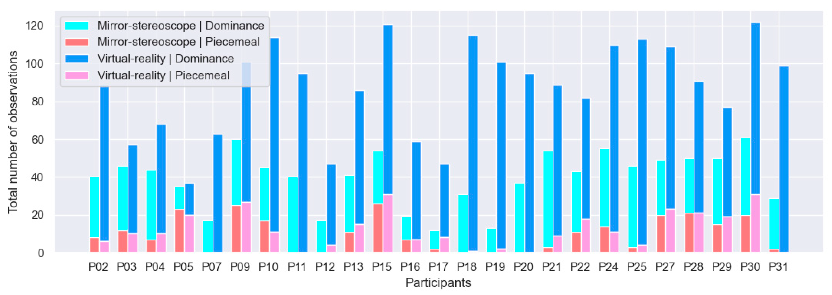
3.1.1. Participant Responses

Figure 8 shows all datasets prior to pruning. Figure 9 shows the reduced sample. Seven participants’ datasets were removed from consideration (P00, P01, P06, P14, P08, P23, P26), reducing the sample from n = 32 to n = 25. This resulted in a 21.9% reduction in sample size. In the case of P00 and P14, the datasets were removed due to technical errors that occurred during testing. For P14, the battery of the VR controller ran out midway through testing. For P00, the configuration was not yet properly working (this participant was considered a trial participant). The datasets for P06 and P23 were removed following a logic check to verify that the responses corresponded to the stimuli presented during the trial, i.e., these participants responded with, for example, horizontal observation while they were presented with a vertical and 45% grating pair. The datasets for participants P01, P08, and P26 were removed due to the excessive number of observations reported by these participants—this was likely the result of holding down the controller, despite instructions to refrain from doing so. For subsequent analyses, the reduced sample (n = 25) was used (shown in Figure 10).

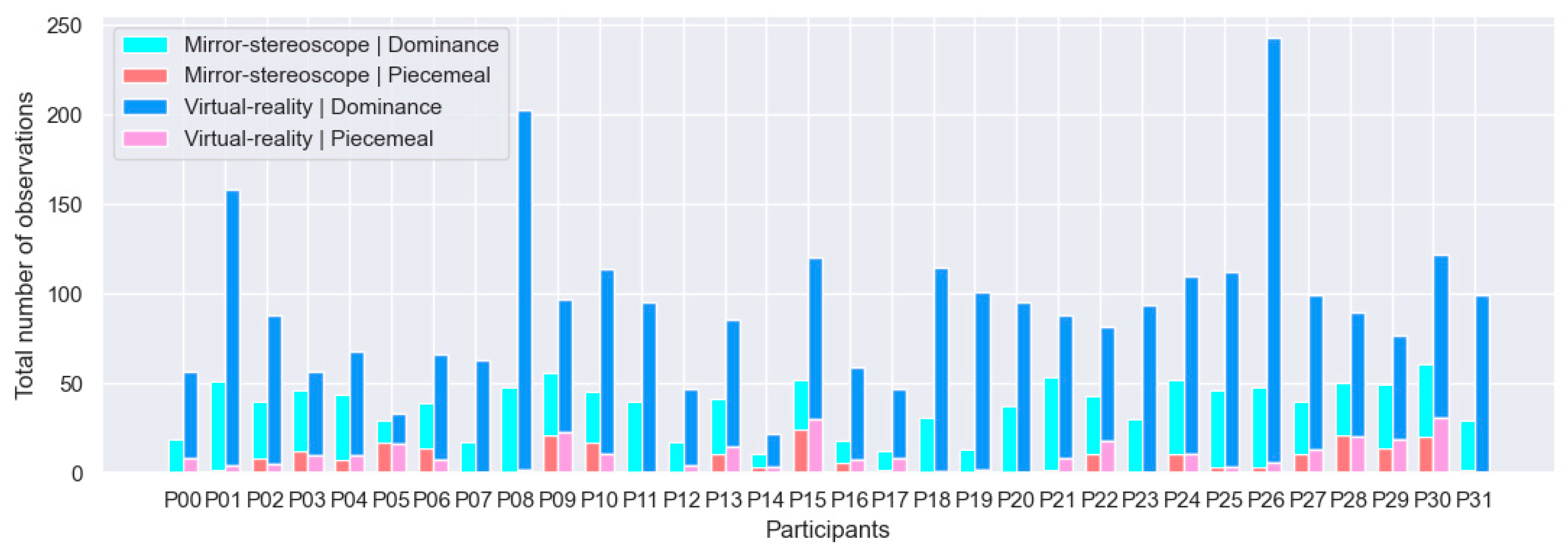
3.1.2. Double-Click Observations

The following assumption was made during the analysis of the button-press responses: Participants would not log consecutive observations of an identical dominance response. Each observation either needed to be followed by a different directional observation or by another observation of piecemeal rivalry. This was the only sequence of observations that can logically constitute alternating stable states. Identical consecutive loggings of observations of dominance were assumed to be erroneous double-click events. See Figure 11 for an analysis of the double-click events. There was a total of 470 double-click events, with the distribution shown in

Table 1. Distribution of double-click events across the mirror-stereoscope and VR experiments for the respective observations (i.e., dominance and non-dominance).

Experiment	Response	Count
Mirror stereoscope	Piecemeal	27
Mirror stereoscope	Dominance	58
VR	Piecemeal	23
VR	Dominance	362

.

Repeated observations of piecemeal rivalry were considered to be possible since alternating states of piecemeal rivalry can follow each other. Following this analysis, all double clicks of observations of dominance were removed. This resulted in a removal of 470 button-press responses across both experiments. This resulted in a reduction of 4.23% for the mirror-stereoscope experiment and a reduction of 12.6% for the VR experiment. These reductions correspond to the VR experiment reporting roughly three times the number of observations of dominance compared to the mirror-stereoscope experiment.

Figure 9 shows the reduced sample, i.e., after specific participants’ data and double-click events of observations of dominance had been removed.

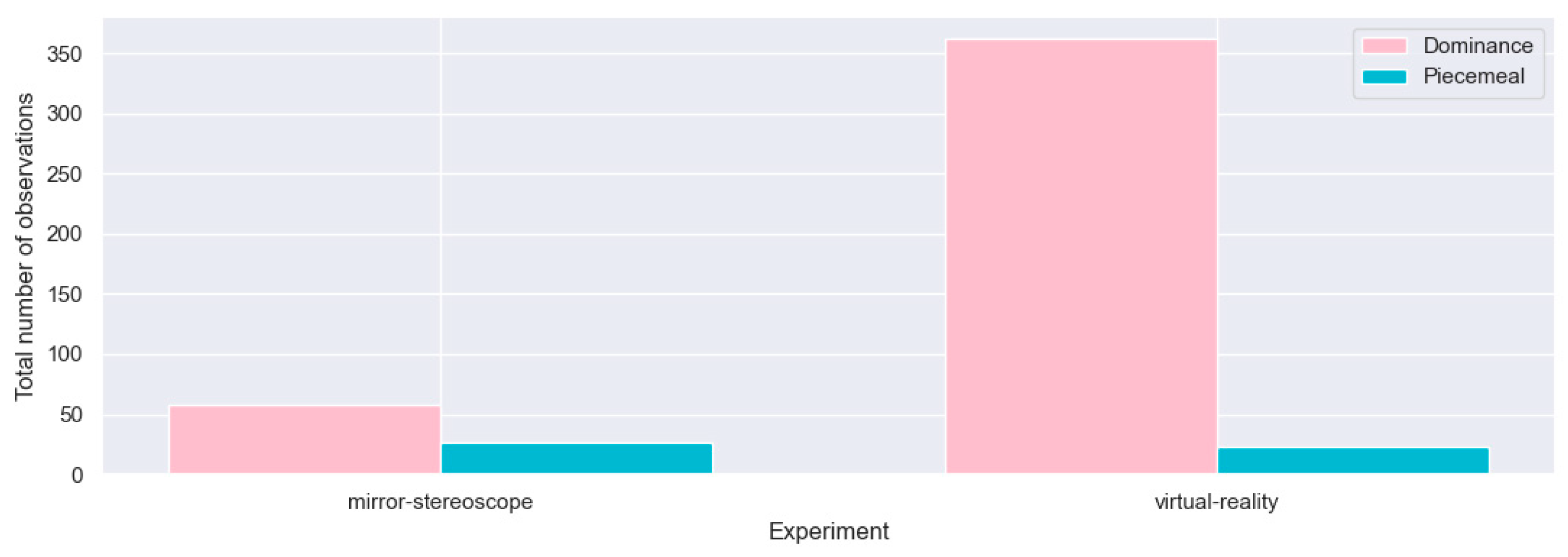
3.2. Inducing BR in Both Experiments

Figure 12 shows the box-and-whisker plot for the number of observations of piecemeal rivalry and dominance for the two experiments across all participants after all erroneous logs had been removed from the data (this includes a removal of double-click events, as well as certain participants’ datasets (Section 3.1.1 and Section 3.1.2)).

Table 2. Sample statistics of an independent t-test evaluating observations of perceptual dominance and piecemeal rivalry for the respective experiments (n = 25).

Experiment	($\overline{x}$, s)d; ($\overline{x}$, s)p *	t-Value	p-Value
Mirror stereoscope	(27.6, 11.0); (13.0, 7.97)	−4.86	<0.0001
VR	(47.7, 14.3); (13.7, 9.20)	−9.41	<0.0001

* ($\overline{x}$, s)_d = observations of perceptual dominance and ($\overline{x}$, s)_p = observations of piecemeal rivalry for both experiments; $\overline{x}$; = mean; s = standard deviation of the sample.

shows the sample statistics comparing the observations of dominance and the observations of non-dominance for the two experiments. For this evaluation, the null hypothesis postulated that the sample data provided no evidence to support that there would be a statistically significant difference between observations of dominance and non-dominance (i.e., between observations of perceptual dominance and piecemeal rivalry) for either the mirror-stereoscope or the VR experiment. In both cases (see Section 3.2.1 and Section 3.2.2), participants were considered as independent samples, an independent-sample t-test was performed to evaluate the relationship between reported observations of dominance and non-dominance for the two experiments [19,28].

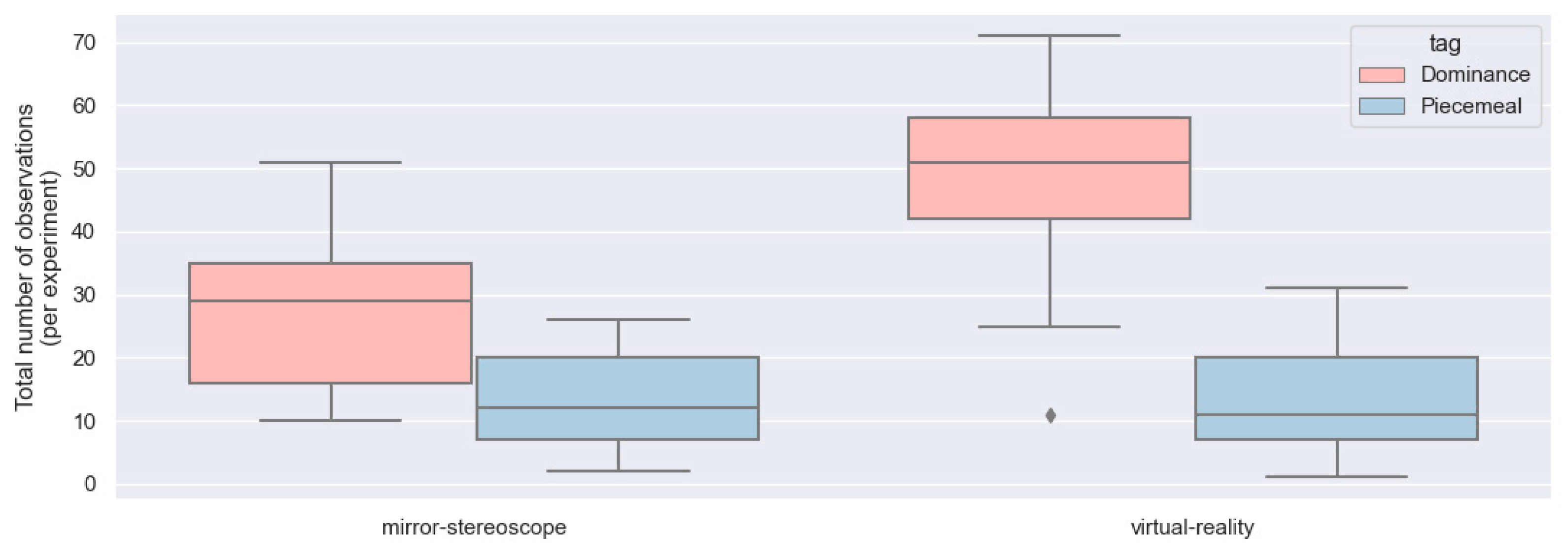
3.2.1. Mirror-Stereoscope Experiment

Figure 10 shows the box-and-whisker plot for the number of observations of perceptual dominance and piecemeal rivalry during the mirror-stereoscope experiment across participants. Equations (1) and (2) show the null hypothesis and alternative hypothesis (where M_d = observations of perceptual dominance for the mirror-stereoscope experiment, and M_p = observations of piecemeal rivalry for the mirror-stereoscope experiment). The null hypothesis states that there is no difference between the mean of the observations of perceptual dominance and the mean of the observations of piecemeal rivalry for this experiment. The consequence of proving the null hypothesis would be a failure to induce BR.

H₀: μM_d = μ_M_p

(1)

H_a: μ_M_d ≠ μ_M_p

(2)

Table 2 shows the sample statistics for the mirror-stereoscope experiment. Performing an independent t-test, the null hypothesis was rejected, with a p-value less than 0.05 (t = −4.86; p < 0.0001), (Table 2). Consequently, there were statistically significantly more observations of perceptual dominance than observations of piecemeal rivalry, i.e., BR with stable vergence was successfully induced.

3.2.2. VR Experiment

The box-and-whisker plot showing the number of observations of perceptual dominance and piecemeal rivalry for the VR experiment across participants can be seen in Figure 10. Equations (3) and (4) show the null hypothesis and alternative hypothesis (where VR_d = observations of perceptual dominance for the VR experiment, and VR_p = observations of piecemeal rivalry for the VR experiment). Similarly, the null hypothesis for the VR experiment states that there is no difference between the mean of the observations of perceptual dominance compared to the mean of the observations of piecemeal rivalry.

H₀: μ_VR_d = μ_VR_p

(3)

H_a: μ_VR_d ≠ μ_VR_p

(4)

Table 2 shows the sample statistics for the VR experiment. Performing an independent t-test, the null hypothesis was rejected for the VR experiment, with a p-value less than 0.05 (t = −9.41; p < 0.0001), (Table 2). There were statistically significantly more observations of perceptual dominance than observations of piecemeal rivalry for the VR experiment, i.e., BR with stable vergence was successfully induced.

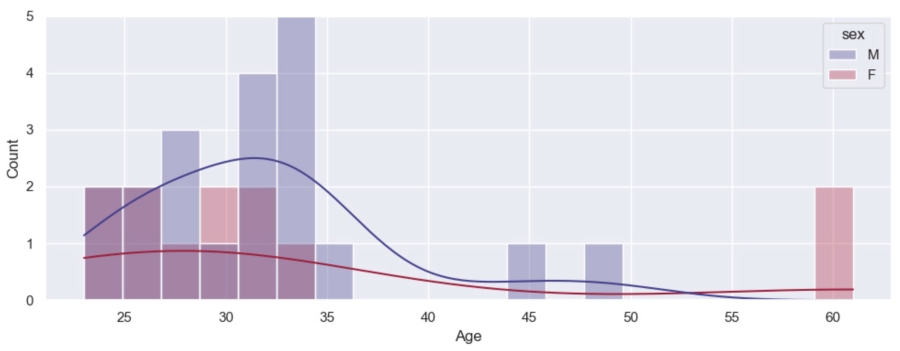
3.3. Statistical Analysis of the Sample

Having established that BR was successfully induced for both experiments, the way BR behaved between the different experiments for the different stimulus pairs needed to be evaluated next. This was evaluated by considering the alternation rate and the observation duration of the two experiments. For this evaluation, the stimulus pairs were divided into three distinct groups. The LD-RD group included stimulus pairs of Gabor patches with gratings at +45°/−45° orientations (i.e., right-diagonal and left-diagonal patches presented to both eyes). The H-V group included stimulus pairs of Gabor patches with gratings at 0°/90° orientations (i.e., horizontal and vertical patches presented to both eyes). The mixed group included the remaining stimulus pairs. Figure 12 and Figure 13 show the box-and-whisker plots of the average alternation rate (per trial) and the average observation duration (in seconds) for the different stimulus pairs for the two experiments across all participants (n = 25). From these graphs, all stimuli showed an approximately normal distribution for the different stimulus groups across the two experiments for both the alternation rates and the observation durations. The box-and-whisker plots depicting the observation durations showed a few outliers.

An ANOVA model, used to evaluate the variance between different normally distributed target groups [19,28], showed statistically significant differences for the alternation rate per trial (F = 25.8; p < 0.0001), as well as the observation duration in seconds (F = 23.8; p < 0.0001), between different stimulus groups for the two experiments. Looking at the R-square values, the model explained 47.2% and 45.2% of the variation in the data for the alternation rate and the observation duration, respectively.

Table 3. ANOVA model statistics for the average alternation rate per trial for the different stimulus groups for the respective experiments across all participants.

Source	DF	F-Value	p-Value
Experiment	1	91.6	<0.0001
Stimulus groups	2	8.1	0.0005
Exp:Stimuli	2	10.6	<0.0001

Exp:Stimuli = interaction between the experiments and the stimulus groups.

and

Table 4. ANOVA model statistics for the observation duration (in seconds) for the different stimulus groups for the respective experiments across all participants.

Source	DF	F-Value	p-Value
Experiment	1	114	<0.0001
Stimulus groups	2	0.10	0.91
Exp:Stimuli	2	2.22	0.11

Exp:Stimuli = interaction between the experiments and the stimulus groups.

show the model statistics for the alternation rate and the observation duration, respectively, and

Table 5. Summary of the statistics for the different variables based on the alternation rate per trial.

Experiment	Stimulus Group	n	Mean ($\overline{x}$)	Standard Deviation (s)
Mirror stereoscope	LD-RD	25	2.98	1.25
Mirror stereoscope	H-V	25	3.22	1.57
Mirror stereoscope	Mixed	25	3.04	1.07
VR	LD-RD	25	8.12	3.94
VR	H-V	25	4.46	1.70
VR	Mixed	25	6.68	1.97

LD-RD = stimulus pairs with −45°/45° orientations; H-V= stimulus pairs with 0°/90° orientations; mixed = remaining stimulus pairs, excluding LD-RD and H-V stimulus pairs; $\overline{x}$ = mean; s = standard deviation of the sample (n = 25).

and

Table 6. Summary of the statistics for the different variables based on the observation duration (in seconds).

Experiment	Stimulus Group	n	Mean ($\overline{x}$)	Standard Deviation (s)
Mirror stereoscope	LD-RD	25	3.38	1.54
Mirror stereoscope	H-V	25	2.79	1.39
Mirror stereoscope	Mixed	25	3.03	1.43
VR	LD-RD	25	0.80	1.04
VR	H-V	25	1.21	0.88
VR	Mixed	25	0.97	0.51

LD-RD = stimulus pairs with −45°/45° orientations; H-V= stimulus pairs with 0°/90° orientations; mixed = remaining stimulus pairs, excluding LD-RD and H-V stimulus pairs; $\overline{x}$ = mean; s = standard deviation of the sample (n = 25)

show the summary statistics for the different dependent groups for the alternation rate and observation duration, respectively. The statistical power for the dependent groups can be found in

Table 7. Statistical power for the different dependent groups (alpha = 0.05; nominal power = 0.8).

Dependent	Source	n Total	Power
Obs. duration	Experiment	25	>0.999
Obs. duration	Stimulus groups	25	0.06
Obs. duration	Exp:Stimuli	25	>0.999
Alt. rate	Experiment	25	>0.999
Alt. rate	Stimulus groups	25	>0.999
Alt. rate	Exp:Stimuli	25	>0.999

Obs. duration = observation duration (in seconds); Alt. rate = alternation rate per trial; Exp:Stimuli = interaction between the experiments and the stimulus groups.

. Table 7 shows that all experimental groups (n = 25) showing statistically significant differences had a statistical power of > 0.999. In the case where the different stimulus groups did not show a statistically significant difference for the alternation rate per trial, the statistical power was smaller than 80% (see Table 7). From the power analysis, proving a statistically significant difference between the different stimulus groups for the alternation rate per trial would require a much larger sample. However, similar BR studies typically reported on response data of ~25–35 participants [19].

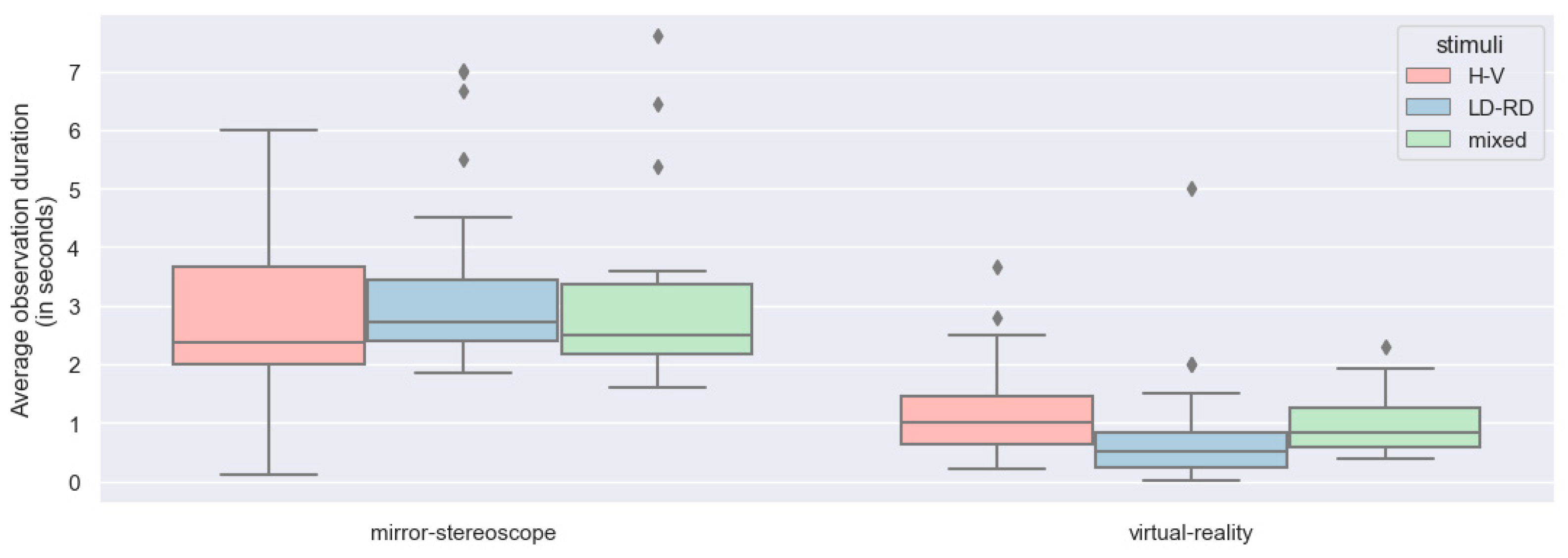
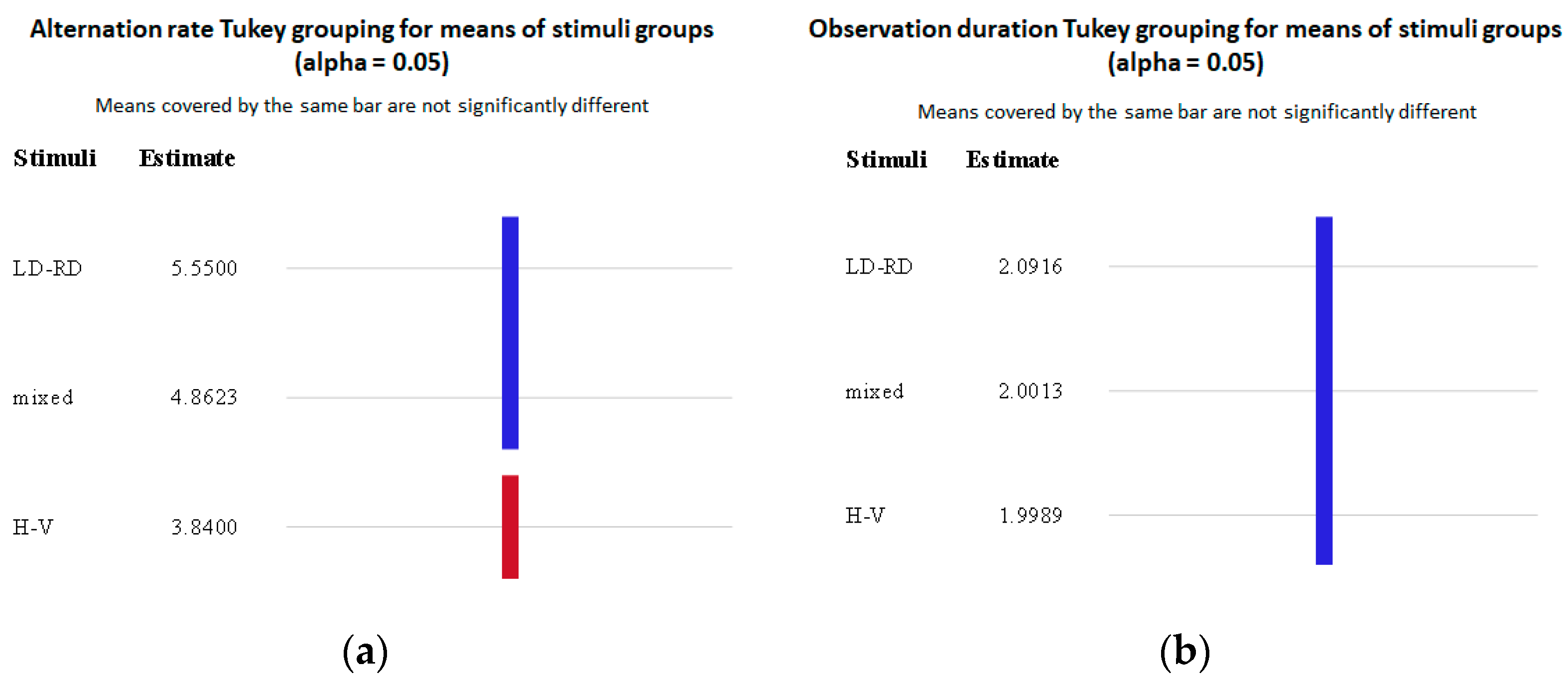
3.3.1. Evaluating the Stimulus Pairs

It was important to consider how BR behaved for the different stimulus pairs for the respective experiments, seeing as most previous studies only considered LD-RD and H-V stimuli when studying BR. The different stimulus pairs were compared by considering the observation duration and the alternation rate for both experiments separately across all participants (n = 25).

Table 8. Sample statistics for the average alternation rate per trial for the different stimulus groups for the respective experiments across all participants.

Stimulus Group	Mean ($\overline{x}$)	Standard Deviation (s)
LD-RD	5.55	3.89
H-V	3.84	1.74
Mixed	4.86	2.42

LD-RD = stimulus pairs with −45°/45° orientations; H-V= stimulus pairs with 0°/90° orientations; mixed = remaining stimulus pairs, excluding LD-RD and H-V stimulus pairs; $\overline{x}$ = mean; s = standard deviation of the sample (n = 25).

and

Table 9. Sample statistics for the average observation duration (in seconds) for the different stimulus groups for the respective experiments across all participants (n = 25).

Stimulus Group	Mean ($\overline{x}$)	Standard Deviation (s)
LD-RD	2.09	1.84
H-V	1.99	1.40
Mixed	2.00	1.49

LD-RD = stimulus pairs with −45°/45° orientations; H-V= stimulus pairs with 0°/90° orientations; mixed = remaining stimulus pairs, excluding LD-RD and H-V stimulus pairs; $\overline{x}$ = mean; s = standard deviation of the sample (n = 25).

show the summary statistics for the alternation rate and the observation duration for the different stimulus pairs for the two experiments.

ANOVA was performed to evaluate the differences between the stimulus groups based on the alternation rate per trial and the observation duration (in seconds). Considering the alternation rate, the model showed statistically significant differences between the different stimulus groups, with a p-value smaller than 0.05 (F = 8.10; p < 0.0001) (Table 3). However, there was no statistically significant difference between the stimuli in terms of observation duration (F = 0.01; p = 0.91) (Table 5).

Figure 14 shows the Tukey post hoc test groupings for the mean of the stimulus groups for the alternation rate (Figure 14a) and the observation duration (Figure 14b). Figure 14a more clearly shows the difference between the alternation rates for the different stimuli groups—a difference was observed between the H-V pairings and the rest of the stimulus pairs.

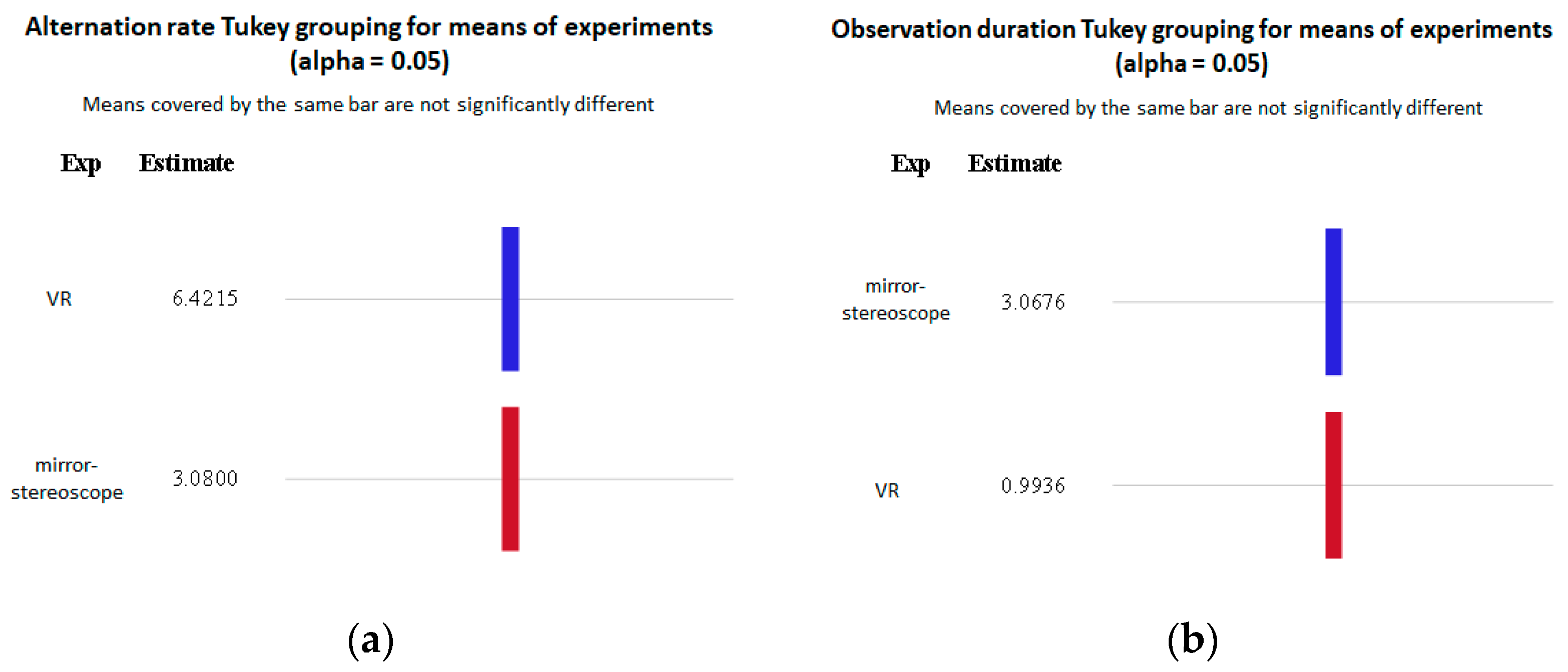
3.3.2. Evaluating the Different Experiments

Next, the differences between the performance of the mirror-stereoscope and VR experiments were evaluated.

Table 10. Sample statistics for the average alternation rate per trial for the different stimulus groups for the respective experiments across all participants.

Experiment	Mean ($\overline{x}$)	Standard Deviation (s)
Mirror stereoscope	3.08	1.30
VR	6.42	3.09

$\overline{x}$ = mean; s = standard deviation of the sample (n = 25).

and

Table 11. Sample statistics for the average observation duration (in seconds) for the different stimulus groups for the respective experiments across all participants (n = 25).

Experiment	Mean ($\overline{x}$)	Standard Deviation (s)
Mirror stereoscope	3.07	1.46
VR	0.99	0.84

$\overline{x}$ = mean; s = standard deviation of the sample.

show a summary of the statistics for the alternation rate and the observation duration for the different stimulus pairs for the two experiments.

ANOVA was performed to evaluate the differences between the experiments based on the alternation rate per trial and the observation duration (in seconds). In both cases, the model showed statistically significant differences between the experiments, with p-values smaller than 0.05 (alternation rate: F = 91.6, p < 0.0001; observation duration: F = 114, p < 0.0001) (Table 3 and Table 5). Figure 15 shows the Tukey post hoc test groupings for the mean of the experiments for the alternation rate (Figure 15a) and the observation duration (Figure 15b). In both cases, significant differences were observed between the mirror stereoscope and VR experiments.

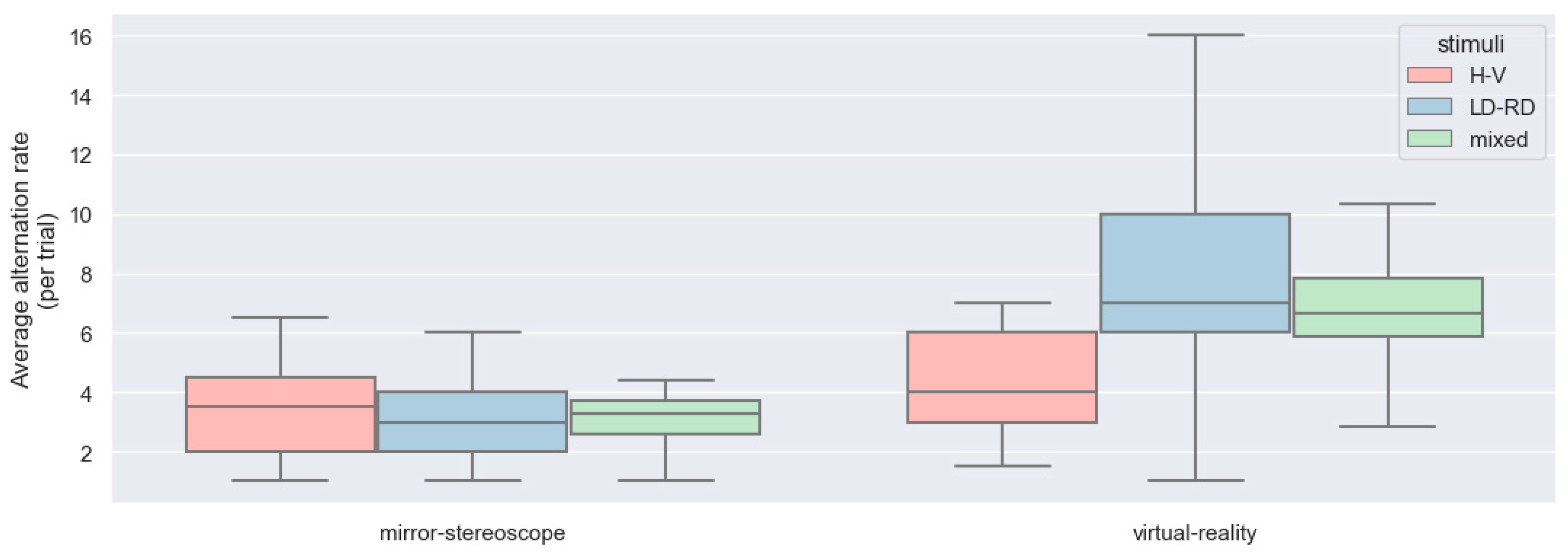
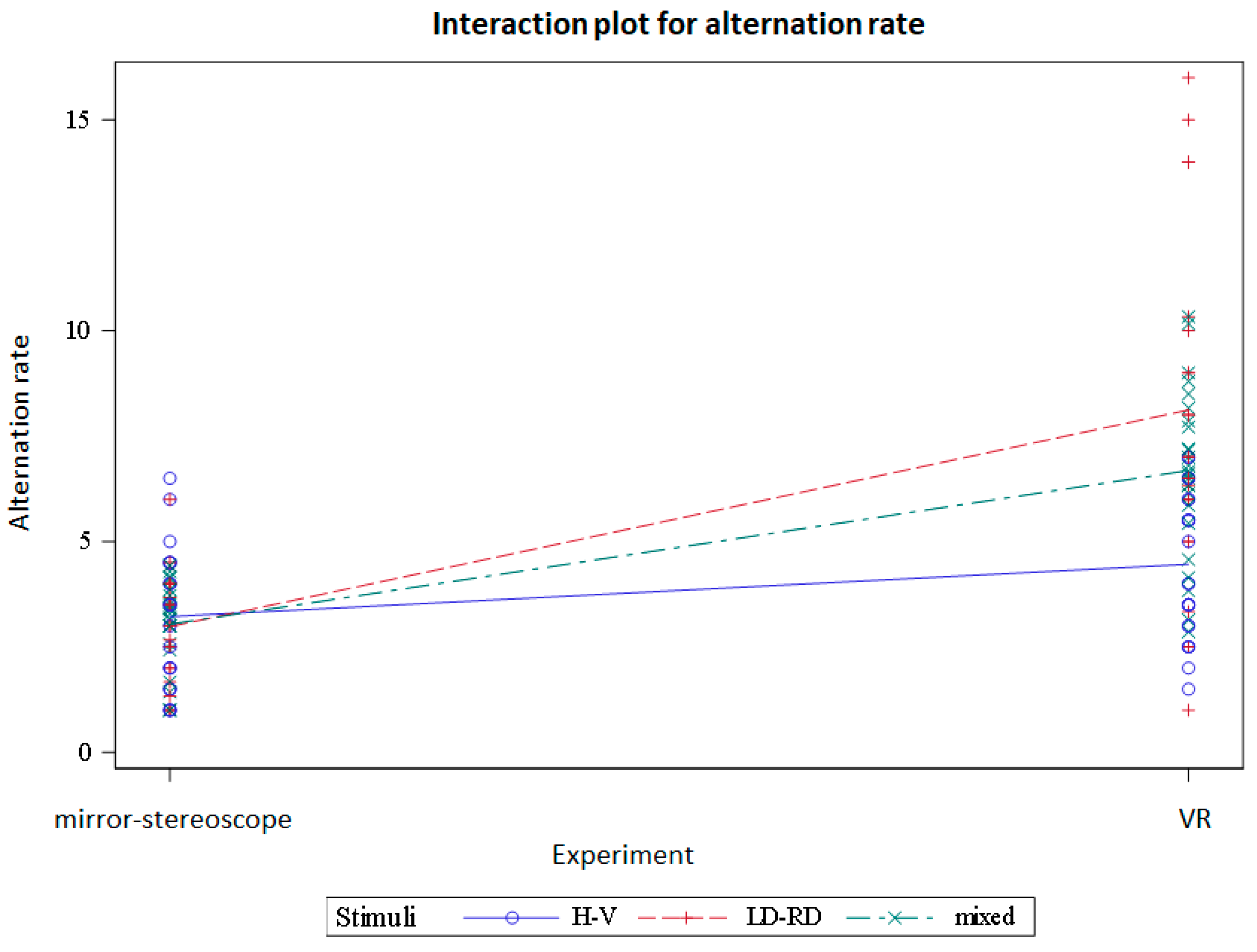
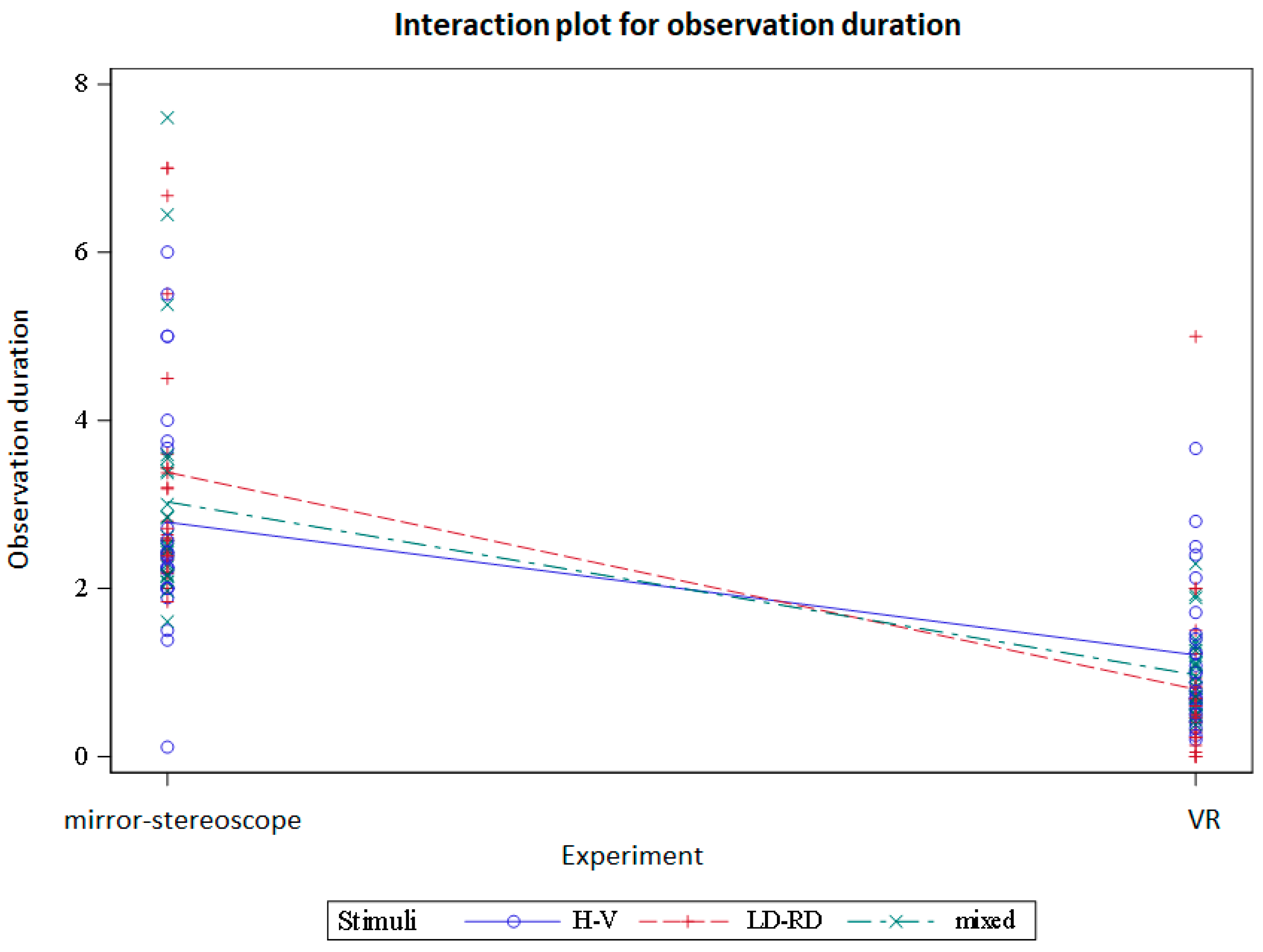
3.3.3. Visualising the Interaction between the Different Experiments and Stimulus Groups

Figure 16 and Figure 17 show the interactions between the stimulus groups and the experiments based on the alternation rate and observation duration, respectively.

4. Discussion

Evaluating the two experiments, the results show that BR with stable vergence was successfully induced in both the mirror-stereoscope and VR experiments. In both experiments there were significantly more visual states of dominance than non-dominance. Moreover, although the VR experiment performed similarly in terms of observations of piecemeal rivalry, there were significantly more observations of dominance during the VR experiment. An increase in the number of observations of piecemeal rivalry and perceptual dominance in the VR experiment could suggest that the VR experiment presented with less stable visual states than the mirror-stereoscope experiment; however, considering the VR headset more frequently switched between different observations of dominance, further evaluation of the neurophysiological data for the two experiments is needed to better understand this difference.

The literature shows that the process responsible for selection (or predominance) differs from the process responsible for alternations [10], all of which involve multiple brain regions. Therefore, for subsequent analysis comparing the performance of the different stimuli and the experiments, the observation duration and alternation rate were evaluated.

The different stimuli groups showed differences in alternation rate but not in observation duration. The difference in alternation rate occurred between the horizontal/vertical stimulus pairing but not the other stimulus pairs. Comparing the dominance durations and the alternation rate per trial between the two experiments, there were statistically significant differences between the mirror stereoscope and the VR headset for both the dominance durations and the alternation rates. The results showed a significant decrease in dominance duration and an increase in alternation rate for the VR headset. Looking at the interactions between the stimuli and the two experiments, there were differences for both the alternation rates and the observation durations.

The differences between the two experiments suggest that the VR headset might perform better than the conventional mirror stereoscope at inducing and maintaining continuous alternating states of dominance/suppression during BR. The alternation rate reflects the inherent dynamic behaviour of neural activity in the visual cortex [29]. Research has found that higher alternation rates during BR are associated with healthy neurological behaviour [29]. Other studies suggest that differences in alternation rates during BR are indicative of differences in bottom-up and top-down visual processing, where a slower alternation rate is associated with lower levels of visual detail during ongoing thought [30]. This could explain why BR induced in a head-mounted display led to a decrease in observation duration and an increase in alternation rate; since the task was completed in visual isolation, fewer external visual sources of information may have resulted in a greater level of focus while performing the visual task. However, research also suggests that the durations of subsequent observations are statistically independent from one another [9]. Further analysis of the neurological effects of BR during these two experiments is required to provide a more comprehensive understanding of the comparative performance of these two methods. It may be prudent to compare the electroencephalographic data of the two experiments for a more conclusive review of the differences and similarities between the two experiments. Moreover, it may be necessary to evaluate whether the different ways in which participants recorded their observations (using a controller for the VR experiment and using a keyboard for the mirror-stereoscope experiment) adversely influenced the results. It should also be noted as a limitation of this study that the IPD was not adjusted in the VR headset for participants—this may have adversely influenced the stability of perceptual dominance during BR in the VR headset.

In conclusion, this study was able to show that BR can be successfully induced using a virtual-reality head-mounted display, and that VR can potentially be used as an effective alternative method to induce and study BR.

References

1. Wheatstone, C. Contributions to the physiology of vision—Part I: On some remarkable and hitherto unobserved phenomena of binocular vision. Philos. Trans. R. Soc. B Biol. Sci. 1838, 128, 371–394. [Google Scholar]
2. Von Helmholtz, H. Handbuch der Physiologischen Optik; L. Voss: Leipzig, Germany, 1867. [Google Scholar]
3. Leopold, D.A.; Logothetis, N.K. Activity changes in early visual cortex reflect monkeys’ percepts during binocular rivalry. Nature 1996, 379, 549–553. [Google Scholar] [CrossRef]
4. Lumer, E.D.; Friston, K.J.; Rees, G. Neural Correlates of Perceptual Rivalry in the Human Brain. Science 1998, 280, 1930–1934. [Google Scholar] [CrossRef] [PubMed] [Green Version]
5. Logothetis, N.K.; Schall, J.D. Neuronal Correlates of Subjective Visual Perception. Science 1989, 245, 761–763. [Google Scholar] [CrossRef]
6. Blake, R.; O’Shea, R.P. Binocular rivalry. In The Curated Reference Collection in Neuroscience and Biobehavioral Psychology; Elsevier: Amsterdam, The Netherlands, 2016. [Google Scholar]
7. Blake, R.; O’Shea, R.P.; Mueller, T.J. Spatial zones of binocular rivalry in central and peripheral vision. Vis. Neurosci. 1992, 8, 469–478. [Google Scholar] [CrossRef] [PubMed]
8. Fox, R.; Herrmann, J. Stochastic properties of binocular rivalry alternations. Percept. Psychophys. 1967, 2, 432–436. [Google Scholar] [CrossRef]
9. Alais, D.; Blake, R. (Eds.) Binocular Rivalry; The MIT Press: Cambridge, MA, USA, 2004. [Google Scholar] [CrossRef]
10. Blake, R.; Logothetis, N.K. Visual competition. Nat. Rev. Neurosci. 2002, 3, 13–21. [Google Scholar] [CrossRef]
11. Logothetis, N.K.; Leopold, D.A.; Sheinberg, D.L. What is rivalling during binocular rivalry? Nature 1996, 380, 621–624. [Google Scholar] [CrossRef]
12. Lee, S.-H.; Blake, R. Rival ideas about binocular rivalry. Vis. Res. 1999, 39, 1447–1454. [Google Scholar] [CrossRef] [Green Version]
13. Blake, R.; Fox, R. Binocular rivalry suppression: Insensitive to spatial frequency and orientation change. Vis. Res. 1974, 14, 687–692. [Google Scholar] [CrossRef]
14. Crick, F.; Koch, C. Toward a neurobiological theory of consciousness. Semin. Neurosci. 1990, 2, 263–275. [Google Scholar]
15. Jack, B.N. Binocular Rivalry for Beginners. i-Perception 2012, 3, 503–504. [Google Scholar] [CrossRef] [PubMed] [Green Version]
16. Carmel, D.; Arcaro, M.; Kastner, S.; Hasson, U. How to Create and Use Binocular Rivalry. J. Vis. Exp. 2010, 45, e2030. [Google Scholar] [CrossRef] [Green Version]
17. Andrews, T.J.; Purves, D. Similarities in normal and binocularly rivalrous viewing. Proc. Natl. Acad. Sci. USA 1997, 94, 9905–9908. [Google Scholar] [CrossRef] [PubMed] [Green Version]
18. Bayle, E.; Guilbaud, E.; Hourlier, S.; Lelandais, S.; Leroy, L.; Plantier, J.; Neveu, P. Binocular rivalry in monocular augmented reality devices: A review. Proc. SPIE 2019, 11019, 110190H. [Google Scholar] [CrossRef]
19. Alpers, G.W.; Ruhleder, M.; Walz, N.; Mühlberger, A.; Pauli, P. Binocular rivalry between emotional and neutral stimuli: A validation using fear conditioning and EEG. Int. J. Psychophysiol. 2005, 57, 25–32. [Google Scholar] [CrossRef]
20. Stanley, J.; Carter, O.; Forte, J. Color and Luminance Influence, but Can Not Explain, Binocular Rivalry Onset Bias. PLoS ONE 2011, 6, e18978. [Google Scholar] [CrossRef] [Green Version]
21. Carrasco, M.; McElree, B. Covert attention accelerates the rate of visual information processing. Proc. Natl. Acad. Sci. USA 2001, 98, 5363–5367. [Google Scholar] [CrossRef] [Green Version]
22. Ernst, U.; Denève, S.; Meinhardt, G. Detection of gabor patch arrangements is explained by natural image statistics. BMC Neurosci. 2007, 8, P154. [Google Scholar] [CrossRef] [Green Version]
23. Mathôt, S. Gabor Patch Generator. 2019. Available online: https://www.cogsci.nl/gabor-generator (accessed on 27 February 2022).
24. Wilson, C.J.; Soranzo, A. The Use of Virtual Reality in Psychology: A Case Study in Visual Perception. Comput. Math. Methods Med. 2015, 2015, 151702. [Google Scholar] [CrossRef] [Green Version]
25. Epic Games. Unreal Engine [Internet]. 2019. Available online: https://www.unrealengine.com (accessed on 14 February 2023).
26. Ling, S.; Hubert-Wallander, B.; Blake, R. Detecting contrast changes in invisible patterns during binocular rivalry. Vis. Res. 2010, 50, 2421–2429. [Google Scholar] [CrossRef] [PubMed] [Green Version]
27. Hernández-Lorca, M.; Sandberg, K.; Kessel, D.; Fernández-Folgueiras, U.; Overgaard, M.; Carretié, L. Binocular rivalry and emotion: Implications for neural correlates of consciousness and emotional biases in conscious perception. Cortex 2019, 120, 539–555. [Google Scholar] [CrossRef] [PubMed]
28. Wackerly, D.D.; Mendenhall, W.; Scheaffer, R.L. Mathematical Statistics with Applications, 7th ed.; Thomson Learning, Inc.: Chicago, IL, USA, 2008; Available online: http://fvela.files.wordpress.com/2012/01/mathematical_statistics_with_applications1.pdf (accessed on 27 February 2022).
29. Ye, X.; Zhu, R.-L.; Zhou, X.-Q.; He, S.; Wang, K. Slower and Less Variable Binocular Rivalry Rates in Patients With Bipolar Disorder, OCD, Major Depression, and Schizophrenia. Front. Neurosci. 2019, 13, 514. [Google Scholar] [CrossRef] [Green Version]
30. Ho, N.S.P.; Baker, D.; Karapanagiotidis, T.; Seli, P.; Wang, H.T.; Leech, R.; Bernhardt, B.; Margulies, D.; Jefferies, E.; Smallwood, J. Missing the forest because of the trees: Slower alternations during binocular rivalry are associated with lower levels of visual detail during ongoing thought. Neurosci. Conscious. 2020, 2020, niaa020. [Google Scholar] [CrossRef] [PubMed]
Figure 1. Perceptual dominance during a BR experiment showing alternation between suppression/dominance states.
Mca 28 00077 g001
Figure 2. Visual example of piecemeal rivalry during BR showing an overlay of stimuli presented to both visual fields.
Mca 28 00077 g002
Figure 3. Four different Gabor patches at different orientations used during the BR tasks [23]: (a) right-diagonal orientation; (b) left-diagonal orientation; (c) horizontal orientation; (d) vertical orientation.
Mca 28 00077 g003
Figure 4. Conventional mirror stereoscope fusing dichoptic vision to induce BR.
Mca 28 00077 g004
Figure 5. Demographic distribution of the sample in terms of age and sex.
Mca 28 00077 g005
Figure 6. Experimental setups and response mappings for (a) conventional BR setup using a stereoscope, computer screen, and standard keyboard; (b) novel setup using a VR headset and right controller. Written permission was obtained from the individuals shown in these photos.
Mca 28 00077 g006
Figure 7. Typical experimental sequence showing rivalrous stimuli interspersed by a 5 s countdown screen; each stimulus pair was presented for 10 s.
Mca 28 00077 g007
Figure 8. Cumulative bar plots for all participants’ (n = 32) observations of dominance and non-dominance for the mirror-stereoscope and VR experiments.
Mca 28 00077 g008
Figure 9. Cumulative bar plots for the reduced sample’s (n = 25) observations of dominance and non-dominance for the mirror-stereoscope and VR experiments.
Mca 28 00077 g009
Figure 10. Box-and-whisker plot for the observations of piecemeal rivalry and dominance for both experiments across all participants (n = 25).
Mca 28 00077 g010
Figure 11. Bar plots of all double-click observations of dominance and non-dominance across the reduced participant dataset (n = 25).
Mca 28 00077 g011
Figure 12. Box-and-whisker plots for the alternation rates per trial between different stimulus pairs for both experiments across all participants (n = 25).
Mca 28 00077 g012
Figure 13. Box-and-whisker plots for the observation duration (in seconds) between different stimulus pairs for both experiments across all participants (n = 25).
Mca 28 00077 g013
Figure 14. Tukey grouping of statistically significant differences for means of stimulus groups (alpha = 0.05) for the (a) alternation rate per trial and the (b) observation duration (in seconds).
Mca 28 00077 g014
Figure 15. Tukey grouping of statistically significant differences for means of experiment groups (alpha = 0.05) for the (a) alternation rate per trial and the (b) observation duration (in seconds).
Mca 28 00077 g015
Figure 16. Interactions between the mirror-stereoscope and VR experiments for the difference stimulus groups based on the alternation rate per trial.
Mca 28 00077 g016
Figure 17. Interactions between the mirror-stereoscope and VR experiments for the difference stimulus groups based on the observation duration (in seconds).
Mca 28 00077 g017