Abstract
The inverse finite element method is a technique that can be used for material model parameter characterization. The literature shows that this approach may get caught in the local minima of the design space. These local minimum solutions often fit the material test data with small errors and are often mistaken for the optimal solution. The problem with these sub-optimal solutions becomes apparent when applied to different loading conditions where significant errors can be witnessed. The research of this paper presents a new method that resolves this issue for Mooney–Rivlin and builds on a previous paper that used flat planes, referred to as hyperplanes, to map the error functions, isolating the unique optimal solution. The new method alternatively uses a constrained optimization approach, utilizing equality constraints to evaluate the error functions. As a result, the design space’s curvature is taken into account, which significantly reduces the amount of variation between predicted parameters from a maximum of % in the previous paper down to % in the results presented here. The results of this study demonstrate that the new method not only isolates the unique optimal solution but also drastically reduces the variation in the predicted parameters. The paper concludes that the presented new characterization method significantly contributes to the existing literature.
1. Introduction
Several tests have become standardized in characterizing hyperelastic material models, such as the Mooney–Rivlin model. Well-established examples of these tests are uniaxial tension, planar tension, equibiaxial tension, uniaxial compression, and bulge tests [1,2]. The coefficients of the constitutive material are determined with physical test data obtained from these tests. A common tool for fitting the coefficients is least squares regression (curve fitting) as demonstrated by research groups [1,2,3,4,5,6]. The curve-fitting approach is considered a direct method for characterization. The limitation of the direct approach is the requirement of an analytical solution to recreate a stress–stretch curve. In cases where the sample geometry becomes relatively complex, an analytical solution may either be too difficult to determine or may not exist. It is then not possible to apply the direct method approach. In these situations, the inverse finite element method must be applied. This approach is also referred to as the finite element method updating method or FEMU.
The Inverse FE approach is not without its own problems, as demonstrated by several research groups [4,6,7,8,9,10,11,12] where the solutions are often non-unique. These non-unique solutions fit the test data with identical error levels to the actual solution, as if the model has been successfully characterized. The differences in these solutions become evident when these models are applied to different load cases resulting in significant errors [4,13]. A paper by Nicholson [7] demonstrated that even in cases of linear elasticity, where direct well-posed problems have a unique solution, the corresponding inverse problem may not. There appeared to be a gap in the literature for handling these non-unique solutions, which prompted research into what key factors are present in this problem.
In previous research [14], it was hypothesized that the non-unique solutions were caused by local minima scattered throughout the design space. To gain insight into the distribution of local minima, error functions between predicted and measured material behavior from a non-standard indentation load case (depicted in Figure 1) was used to sample different areas of the design space. The non-standard test was chosen since the deformation is relatively complex and would contain all material behavioral aspects obtained from the material standard tests in one test case. It is important to note the reference frame indicated in Figure 1, as this will be used throughout the paper. The error functions for surface deformation and indentation force showed a clear pattern to the local minima. The data used in the investigation were from a simulated experiment. Stand-in experimental data were extracted from a relatively high element density finite element model. The investigation was focused on evaluating fundamental behavior and not factors such as experiment noise, incomplete datasets, and other aspects, which is why this type of synthetic data was used.
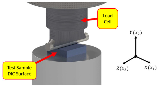
Figure 1.
Indentation test for collecting both full-field digital image correlation (DIC) data and indentation force data. The indenter, test sample, load cell, and base plate are shown.
The results of the design space sampling investigations are presented in Figure 2 and Figure 3. In these figures, red areas indicate a high error, while the blue areas, which correspond to the locations of local minima, represent low error and are of particular interest in this study. After examining these areas of low error in both datasets, it became clear that there exists an identifiable pattern to the local minima rather than being randomly dispersed. Figure 2a displays all the sample points for absolute indentation force error, with the error magnitude for the point represented in color. In Figure 2b, which has the high error points removed, as they are not of interest to the investigation, a strong correlation is evident between the constitutive model parameters and indentation force error. Fitting a flat plane through these filtered data points using linear regression resulted in an score of 0.998, indicating a high degree of fit.
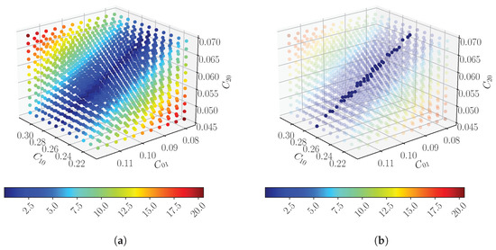
Figure 2.
Absolute indentation force error plots of the sampled design space: (a) showing all the sample points, (b) highlighting the low error region of the design space.
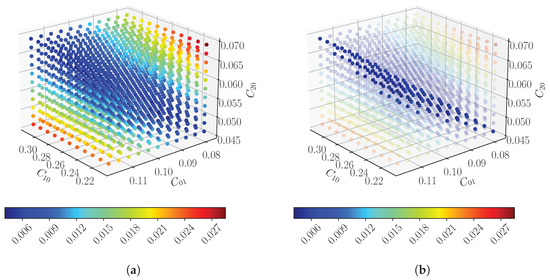
Figure 3.
Displacement field RMSE error plots of the sampled design space: (a) showing all the sample points, (b) highlighting the low error region of the design space.
Similar to the indentation force error results, the results for the displacement field error are depicted in Figure 3a, where blue points indicate the low error region. Figure 3b shows the filtered points for this region, which also reveal a clear correlation between low error and the constitutive model parameters. Fitting a flat plane to perform a regression analysis on these points resulted in an value of 0.941, indicating a high level of fit. Comparing Figure 2b and Figure 3b, it is clear that the two regions have different relationships with the constitutive model parameters. Further investigation revealed that these regions, which are referred to as hyperplanes in [14], rotate around the correct solution. The rotation was found to be dependent on the loading of the sample. Based on these findings, a method was developed to capture this rotation and isolate unique solutions for the Mooney–Rivlin material model. It should be noted that the results of the previous paper [14] were evaluated only on simulated data, and the method’s applicability to physical data remains uncertain, which the research of this paper aims to resolve. Additionally, it was found that the low-error regions were not perfectly flat but had a slight curvature, although assuming them to be flat near the optimal solution did produce low-error results. These factors motivated the research presented in this paper.
The research presented here expands upon previous studies in [14] by exploring a modified version of the previous hyperplane method on data obtained from physical experiments as opposed to simulated experiments. In an effort to account for the curvature of the design space in areas with low error, the method was modified by replacing the intersecting planes with a constrained optimization approach. The objective function of this modification is the prediction error between the displacement field from a finite element model and a measured displacement field using digital image correlation (DIC). The mapping of local minima using planes was transformed into equality constraints. In doing so, the curvature of the low error regions in the design space is considered. The constraints were based on the prediction error of the indentation force. The presented research aims to demonstrate the repeatability of the modified method when applied to physical test data. The results show that a unique solution can still be obtained when assessed on physical test data through a constrained optimization approach. Additionally, the results were found to be highly repeatable, with limited variation in the predicted outcomes across different characterization runs. Twenty different starting points in the design space were evaluated in total.
2. Materials and Methods
The research in this paper builds upon previous work by using a modified version of the hyperplane method described in [14]. In this study, we modified the method for characterizing the Mooney–Rivlin model, but the most significant difference is the use of new test data. The test data came from a physical experiment that includes several aspects not found in a simulated experiment. The aspects are noise and patches of missing displacement data of random regions that result from the DIC system failing to track those specific regions. This is especially true regarding the full-field displacement data captured by a DIC setup.
2.1. Physical Test
The test sample was made of platinum cure Smooth Sil-950 silicone [15]. Prior to testing, it underwent preconditioning which involved applying three full-depth indentations of 20 . This minimized any Mullins effects [16] and ensured that the sample would exhibit its working material behavior rather than its virgin material characteristics.
The test setup is depicted in Figure 4a,b. Figure 4a shows the main components used to collect the indentation force-displacement data. The load cell used for measuring the force had a capacity of 30 and a noise floor of approximately 1 . The measured indentation forces, which characterized the test sample, ranged from at to 1635 at depth. The load cell error of 1 at the indentation depth would be % and was considered negligible for practical purposes.
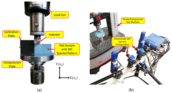
Figure 4.
Indentation test configuration (a) showing the front view highlighting the compression machine key components, (b) showing the DIC configuration.
A calibration plate was used to synchronize the two cameras to the sample location [17] as shown in Figure 4a. Figure 4b depicts the remaining components related to the DIC system. The DIC tracking method used two 5 megapixel cameras placed at a distance of 1 .
After the sample reached the required indentation depth of 20 , 10 stereoscopic images (20 total) were taken at a frequency of 10 Hz. The displacement data were extracted using DaVis 10 [17] software with a step size of 25 and a subset size of 7. Since a stereoscopic DIC method was used, the effect of the cameras not being perpendicular to the test samples’ surface could be ignored [18]. Although the literature states that the effect of the slight camera rotation should be negligible, effort was put into aligning the cameras with the sample.
Once extracted from Davis 10, the DIC coordinate data were processed to ensure the FE model and test data were in the same reference frame. The DIC system requires images of the initial unloaded sample to generate a reference for calculating the displacement field. Rigid body offsets were added to these initial coordinates until the physical test data coordinates matched that of the FE model. Moving the coordinates of the FE model to that of the physical test instead would have the same effect. Rigid body rotations were also implemented for the same purpose, as the Davis 10 software assumes a reference frame, which may be slightly rotated to the desired reference frame.
The measured displacements were averaged across the 10 measurements to minimize the effect of noise. The data were then screened for outliers that resulted from regions of poor correlation by the DIC system. These regions are typically found along the edges of the DIC field, where gradient information is poor and are referred to as edge effects [19]. The edge effects were accounted for by removing all the data points along the perimeter, 1 from the edge, as this was found to be sufficient for the measured dataset. Figure 5 shows all the unfiltered data points from the DIC measurement. This figure highlights three examples of poorly correlated regions with red circles. As expected, these regions are mainly found along the perimeter dataset.
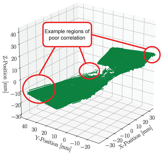
Figure 5.
Unfiltered, full field test data showing each measurement point related to its physical position highlighting regions of poor correlation.
Figure 6 shows the test sample at full indentation depth and the resulting displacement field pattern for each component direction. The test sample had dimensions of 40 × 40 × 120 , and the indenter had a diameter of 25 .
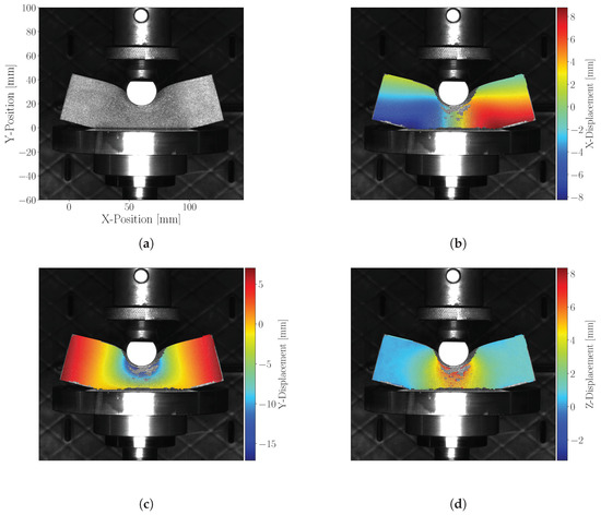
Figure 6.
Raw digital image correlation images showing the component directions: (a) showing the deformed sample, (b) X-displacement component, (c) Y-displacement component, (d) Z-direction component.
The main component of an inverse FE analysis requires an FE model with aspects which are adjusted until the predicted behavior matches the measured behavior with minimal error. The next step is to have physical test data to compare the FE model to.
2.2. Finite Element Model
The FE model must accurately recreate the physical test so that the obtained material parameters accurately reflect the assessed physical material. As seen in Figure 7, the sample geometry has two symmetry planes in conjunction with the cylindrical indenter formed with a geometric surface.
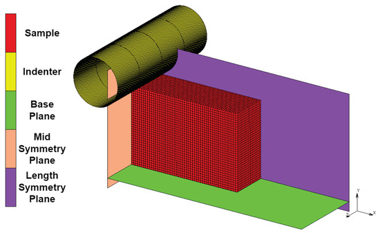
Figure 7.
Finite element model replicating the physical test loading conditions.
2.2.1. Boundary Conditions
To simulate the base plate, which had a touching contact condition applied between it and the test sample nodes, a flat geometric surface was used. This condition allows the nodes to break contact as soon as the reaction force vector is in the opposite direction to the surface while allowing the nodes to move freely along the surface. The indenter was generated from a 25 diameter cylindrical surface with a touching contact condition applied between it and the test sample nodes. The base plate and indenter together restrict any rigid body motion in the Y-direction.
A FE model that uses symmetry was used for this investigation, as it reduces computational costs while obtaining the same level of detail. The FE model uses two symmetry planes, reducing the number of elements in the simulation by a factor of four. The length and mid-symmetry planes indicated in Figure 7 had a touching contact condition applied to them and the sample nodes. However, for symmetry planes in Marc Mentat, nodes on this surface are not allowed to separate, but they can move frictionlessly along the surface [20]. This type of boundary condition can also be created using appropriate displacement constraints. The two symmetry conditions restrict the sample’s rotation in all three directions and restrict motion in the X and Z directions. Therefore, the applied boundary conditions restrict all possible rigid body motions.
2.2.2. Model Friction
In the physical test, artifacts such as friction will be present. To reduce friction as much as possible, all contacting surfaces were given a mirror polish, and silicone grease was applied. The friction coefficient, now significantly reduced, was still unknown. Therefore, a brief study was performed by selecting a range of friction coefficients applied to the FE model’s base plate and indenter, with consideration of the literature-estimated values. This investigation aimed to determine the amount of friction present in the system and the friction coefficient’s effect on the predicted parameters while considering the predicted surface error (objective function) in the inverse FE process. An additional goal of the investigation was to determine if there would be any added benefit to including friction in the FE model. A paper by [21] determined a sliding friction coefficient for a rubber stop on a smooth glass plate coated with silicone oil to between 0.0067 and 0.06. In the FE model of this paper, a Coulomb friction model was chosen. The results of this investigation are shown in Figure 8.
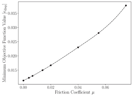
Figure 8.
Friction coefficient effect on objective function .
The results indicate that adding the chosen friction coefficients increased the objective function value. This indicates that the predicted displacement field worsened, implying that these friction coefficients are too large. Further study showed that the positional difference in the design space for friction coefficients less than 0.004 in this test case would result in an absolute mean difference of % in the predicted parameters when compared with the zero friction model estimates. Considering that the friction coefficient in this system, from this study is expected to be close to zero, it was assumed that the additional complexity to the FE model would also have no meaningful difference to the predicted parameters based on the small variation of relatively larger friction coefficients. Therefore, it was decided to exclude friction from the FE model for this investigation.
Evaluating Figure 9, which shows the deformed FE model on the left and the deformed physical sample on the right, we see a close similarity between the two deformations. This similarity confirms that the boundary conditions and contact models accurately simulate the real-life test configuration.
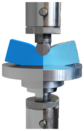
Figure 9.
Finite element model left versus physical sample right at 20 indentation.
2.2.3. Model Mesh
A first-order hexahedral mesh (hex-8) was selected for the FE model due to the simple geometry, as opposed to the second-order tetrahedral elements (tet-10), which had issues with the contact interaction not releasing from the surface.
The choice of hex-8 over tet-10 was also recommended by Hexagon [20], as hex-8 elements are more stable when distorted. Remeshing was not applied in the FE model to allow for node tracking on the surface where the DIC measurements were taken. These surface nodes replicate the full-field dataset that would be obtained through DIC.
Since remeshing was not applied, the element quality and stability were of primary concern. The mesh was exported to MSC Apex, where important mesh characteristics, such as aspect ratio and the Jacobian, were assessed at the full 20 indentation depth. Nearly all elements passed the default assessment criteria, with over % of the mesh having a Jacobian value of 0.9 or higher and % of the meshing having an aspect ratio less than 3.00 at the full indentation depth.
The number of elements used in the mesh was determined through a mesh convergence study, which showed convergence at 19,140 elements.
2.2.4. Indentation Force Extraction
The indentation force could be extracted from either the base plane or the indenter contact body as depicted in Figure 9. The base plane contact body was used in this case. The non-linear solver used in this case was the full Newton–Raphson (Hexagon [20]). This solver updates the system at discrete iterations, resulting in the load-displacement curve having discrete points. A cubic spline fit was used to interpolate between these points so that the indentation force could be requested at any indentation depth.
2.3. Error Functions
With the FE model in place, error functions must be established to compare the physical and predicted material behavior.
2.3.1. Displacement Field Error Function
A weighted root mean square (RMSE) error function was used to compare the measured and predicted displacement fields. The RMSE function produces a single value that represents the overall error for the predicted displacement field. This RMSE function also serves as the objective function for the optimizer in the characterization process.
The displacement field error function calculation consists of three steps. Firstly, an RMSE error score is calculated for each of the three component directions X, Y, and Z (labeled , , and ), represented by , , and , respectively, in Equation (1). The RMSE scores are calculated with Equation (2), where vector contains the measured experiment displacement field, and vector contains the predicted displacement field. In both vectors, i denotes the component direction, and j represents a data point for N total data points:
The next step towards calculating is to sum the vector while dividing each component , , and by the maximum measured displacement in that component direction as shown in Equation (3):
Dividing each RMSE component by the maximum displacement in that direction is performed to mitigate bias introduced in calculating that would otherwise favour larger displacement errors. This is because each component direction will have displacements of varying magnitudes and, correspondingly, RMSE values that differ greatly. The method outlined in Equation (3) proved effective in characterizing complex material models using displacement field data as demonstrated in [22].
The final step towards comparing the measured and predicted displacement fields requires both datasets to be mapped to the same size and order. This requires an interpolation function to map the respective displacements to their corresponding regions between two grid spaces, which are the predicted and measured displacement fields. Each grid space contains XYZ displacements corresponding to their respective XYZ positions. The radial basis function (RBF) was chosen for this task, as it proved to be effective in mapping two grid spaces in [23]. When using the RBF, the positional coordinates for each data point were used, to which the corresponding displacements were mapped. The mapping direction was from the FE model to the DIC displacement field data since the physical test data would have more noise than the dataset from the FE model dataset, which would not be ideal for interpolating. The RBF function was implemented using the Python library SciPy [24].
2.3.2. Indentation Force Error Function
The difference between the measured and predicted indentation force was used to calculate the indentation force error. It is important to note that the two datasets have different resolutions: the FE model generated 18 points between the 0 to 20 indentation, while the measured indentation force curve comprises several thousand points. A cubic spline fit was chosen to calculate the force error at a requested indentation depth. In both the physical and predicted datasets, the cubic splice was fit on indentation depth, with the indentation force being the dependent variable.
The force error function is described by Equation (4). Here, and represent the interpolation functions fitted to the measured (exp) and predicted (sim) indentation force datasets, respectively, and y represents the indentation depth:
2.4. Optimizer and Analysis Details
The final component needed to perform the analysis is an optimizer that will iterate the Mooney–Rivlin coefficients , and to minimize the error between the measured and predicted displacement field subjected to two equality constraints and two inequality constraints. A single variant constrained optimization approach was chosen instead of simultaneously optimizing for both the displacement field and indentation error functions to avoid situations such as Pareto fronts [25].
The chosen optimization algorithm was the modified method of feasible directions (MMFD). The software Design Optimization Tools (DOT) [26] provided the MMFD algorithm. To demonstrate the method’s ability to characterize the Mooney–Rivlin model, an arbitrarily wide range of times the solutions parameter for the and was chosen. However, the parameter range was only since this parameter, which acts as a bulk modulus parameter, significantly impacts the material stiffness for large deformations.
The two equality constraints, represented by Equations (5) and (6), serve to limit the design space to the regions of the hyperplanes discussed in [14] by evaluating the predicted force error at and indentation depths. These equality constraints were implemented in DOT as two equal and opposite inequality constraints with a small tolerance of 1 at both indentation depths:
The two inequality constraints represented by Equations (7) and (8) focus on the material parameters of the Mooney–Rivlin model and ensure that the stability criteria are met [27]:
The goal of this paper is to demonstrate that a unique solution can be determined even with physical test data and that the repeatability of the method used in [14] can be improved with a new formulation. The new approach involves treating the hyperplanes as equality constraints.
To support these focus points, 20 randomly selected starting positions in the design space were generated. The converged optimal results from these 20 starting points can then be investigated to evaluate the robustness of the constrained optimization approach. This will not only indicate if the solutions are unique but also give an indication of repeatability.
The distribution of these starting points and results are shown in Figure 10. The values of these starting points plus additional details are found and summarized in Table A1 of Appendix A.
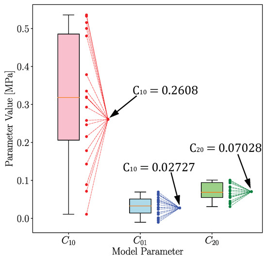
Figure 10.
Optimizer start and end points showing the original distribution with a box and whisker diagram and where the points converged to.
3. Results and Discussion
The start and end positions for each of the 20 optimization runs are illustrated in Figure 10. This figure shows the original distribution of the 20 starting points parameters using box whisker diagrams. The start and end positions for each characterization run of all 20 starting points in the parameter design space are shown in Figure 11. The figure illustrates visually how the points are distributed around the final solution. The numerical values of these points and further details are found in Table A2 of Appendix A.
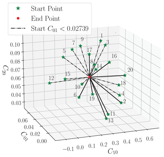
Figure 11.
A 3D plot showing the starting points start (green) and converged end points (red).
The solutions for each optimization run have slight variations in their positions in the design space; the obtained parameters, however, are similar. On average, the parameters differ by 0.08715% for , 0.3159% for , and 0.1614% for . This is a noticeable improvement compared to previous research [14], where the parameters were off by an average of 1.106% for , 1.934% for , and 0.6034% for . On average, there is roughly a 10-fold improvement towards the converged results. The low parameter variation indicates that the problem is well posed and has repeatable results. This variation can be further reduced by applying stricter convergence criteria to the optimizer.
Focusing on the displacement field error, we can see how the optimized model approximates the original displacement field. As seen in Figure 12, the errors in the X and Y direction have similar error levels, while the Z direction shows twice the error. Despite this higher error, the mean error remains at a manageable level of approximately 61 , which is still a good fit considering the large displacements (20 indentation) involved in the physical test. This suggests that the characterized model provides a good approximation of the original displacement field.
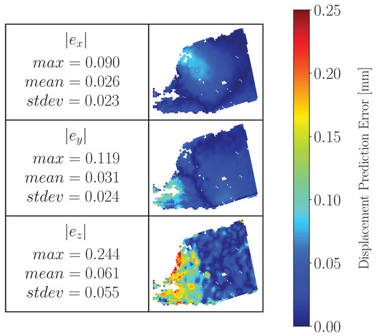
Figure 12.
Displacement field prediction error [mm].
The results of the load-displacement curve comparison between the characterized model and physical test data are shown in Figure 13. The strong positive correlation between the two curves is indicated by a Pearson correlation coefficient of 0.9976 and an RMSE score of from 0 to 20 indentation. However, when measured up until the point of deviation (0 to ), the correlation becomes even stronger with a Pearson coefficient of 0.9997 and a lower RMSE value of . The deviation towards the end of the curves may be due to the reduced-order nature of the Mooney–Rivlin model used in the characterization, and a higher-order version of the model may provide improved results.
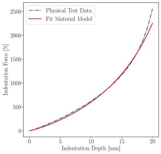
Figure 13.
Force-displacement curve comparing the fitted material model indicated as the average predicted parameters in Table A2 with the experimentally measured force curve.
These results show that the inverse FE characterization of the Mooney–Rivlin model was successful with repeatable and unique results. Regarding the significance of the minor variation in the predicted material behavior, further study would be needed to determine what impact they may have on the overall predicted material behavior and whether the impact is meaningful.
4. Conclusions
In this paper, an inverse finite element analysis was conducted to characterize the Mooney–Rivlin three-parameter model using an indentation loading case. A modification to the hyperplane method established in [14] was applied, which was also able to successfully eliminate the issue of non-unique sub-optimal solutions, a known problem addressed in the literature. The analysis demonstrated through the use of 20 independent starting points that the results were repeatable and unique, even when applied to physical test data. This was confirmed since all starting points converged to the same solution with an average deviation of 0.1882% from the mean predicted set of parameters. This slight variation is not a deficiency in the method but rather a result of the tolerances applied to the optimizer. The slight variation is also a significant improvement on the results of the previous paper, which had an average deviation of 1.934%.
These results highlight how significant the modification to the previous hyperplane method is, which instead treats hyperplanes as equality constraints, which accounted for the continuous curvature of the design space, resulting in reduced variability in the results.
To summarize, the findings of this study demonstrate that a unique solution with repeatable results can be determined using physical experiment data, such as DIC, which are inherently noisy when evaluated with the new method. This provides valuable insight for future researchers facing similar challenges when working with the Mooney–Rivlin three-parameter model, for which the literature may need to provide more information to reduce non-unique solutions. The paper concludes that the present new characterization method significantly contributes to the existing literature by resolving the non-uniqueness problem and providing a method capable of producing highly repeatable results no matter the starting position in the design space.
Author Contributions
Conceptualization, J.D.V.T., M.P.V. and G.V.; Methodology, J.D.V.T.; Software, J.D.V.T.; Formal analysis, J.D.V.T.; Investigation, J.D.V.T.; Resources, M.P.V. and G.V.; Data curation, J.D.V.T.; Writing—original draft, J.D.V.T., M.P.V. and G.V.; Visualization, J.D.V.T.; Supervision, M.P.V. and G.V.; Funding acquisition, M.P.V. and G.V. All authors have read and agreed to the published version of the manuscript.
Funding
This research was funded in part by the National Research Foundation of South Africa (NRF) grant number 129381.
Data Availability Statement
The data presented in this study are available on request from the corresponding author.
Acknowledgments
Computations were performed using the University of Stellenbosch’s HPC1 (Rhasatsha): http://www.sun.ac.za/hpc (accessed on 20 January 2023).
Conflicts of Interest
The authors declare no conflict of interest.
Appendix A
The starting points, as labeled in Section 2.4, are summarized in Table A1 below. The inequality constraints and were omitted, as they do not provide information regarding the results other than whether they meet the stability criteria or not. Variables , and are calculated from Equation (2) and show the RMSE levels for each component direction before they were normalized and added together to form the overall objective function .

Table A1.
All starting points used in the material characterization.
Table A1.
All starting points used in the material characterization.
| Variable | OBJ | ||||||||
|---|---|---|---|---|---|---|---|---|---|
Table A2 contains the same information as Table A1 but for the optimization results. An additional row was added to this table containing each column’s average values.
Table A2.
Converged results of the material characterization.
Table A2.
Converged results of the material characterization.
| Variable | OBJ | ||||||||
|---|---|---|---|---|---|---|---|---|---|
| Average |
References
- Palmieri, G. Mechanical Modeling of Elastomers; LAP LAMBERT Academic Publishing: London, UK, 2010; p. 9. [Google Scholar]
- Kim, N.H. Introduction to Nonlinear Finite Element Analysis; Springer: New York, NY, USA; Heidelberg, Germany; Dordrecht, The Netherlands; London, UK, 2015. [Google Scholar] [CrossRef]
- Bergström, J. Elasticity/Hyperelasticity; William Andrew: San Diego, CA, USA; London, UK; Waltham, MA, USA, 2015; pp. 209–307. [Google Scholar] [CrossRef]
- Ogden, R.; Saccomandi, G.; Sgura, I.; Ogden, R.; Saccomandi, G.; Sgura, I.; Ogden, R.W.; Saccomandi, G.; Sgura, I. Fitting hyperelastic models to experimental data. Open Sci. 2004, 34, 484–502. [Google Scholar] [CrossRef]
- Sasso, M.; Palmieri, G.; Chiappini, G.; Amodio, D. Characterization of hyperelastic rubber-like materials by biaxial and uniaxial stretching tests based on optical methods. Polym. Test. 2008, 27, 995–1004. [Google Scholar] [CrossRef]
- Burman, E.; Hansbo, P.; Larson, M.G. Solving ill-posed control problems by stabilized finite element methods: An alternative to Tikhonov regularization. Inverse Probl. 2018, 34, 035004. [Google Scholar] [CrossRef]
- Nicholson, D.W. On finite element analysis of an inverse problem in elasticity. Inverse Probl. Sci. Eng. 2012, 20, 735–748. [Google Scholar] [CrossRef]
- Suchocki, C.; Jemioło, S. Polyconvex hyperelastic modeling of rubberlike materials. J. Braz. Soc. Mech. Sci. Eng. 2021, 43, 352. [Google Scholar] [CrossRef]
- Seng, J.A.C. Inverse Modelling of Material Parameters for Rubber-like Material: Create a New Methodology of Predicting the Material Parameters Using Indentation Bending Test. Ph.D. Thesis, Liverpool John Moores University, Liverpool, UK, 2015. [Google Scholar]
- Chen, X.; Ogasawara, N.; Zhao, M.; Chiba, N. On the uniqueness of measuring elastoplastic properties from indentation: The indistinguishable mystical materials. J. Mech. Phys. Solids 2007, 55, 1618–1660. [Google Scholar] [CrossRef]
- Alkorta, J.; Martínez-Esnaola, J.; Sevillano, J.G. Absence of one-to-one correspondence between elastoplastic properties and sharp-indentation load–penetration data. J. Mater. Res. 2005, 20, 432–437. [Google Scholar] [CrossRef]
- Turcot, G.; Paquet, D.; Lévesque, M.; Turenne, S. A novel inverse methodology for the extraction of bulk elasto-plastic tensile properties of metals using spherical instrumented indentation. Int. J. Solids Struct. 2022, 236–237, 111317. [Google Scholar] [CrossRef]
- Murdock, K.; Martin, C.; Sun, W. Characterization of mechanical properties of pericardium tissue using planar biaxial tension and flexural deformation. J. Mech. Behav. Biomed. Mater. 2018, 77, 148–156. [Google Scholar] [CrossRef] [PubMed]
- Van Tonder, J.D.; Venter, M.P.; Venter, G. Using Full Field Data to Produce a Single Indentation Test for Fully Characterising the Mooney Rivlin Material Model. MATEC Web Conf. 2021, 347, 00029. [Google Scholar] [CrossRef]
- SMOOTH-ON. Smooth-Sil® Series. 2021. Available online: https://www.amtcomposites.co.za/wp-content/uploads/2021/05/SMOOTH-SIL_SERIES_TB.pdf (accessed on 31 January 2022).
- Yan, L.; Dillard, D.A.; West, R.L.; Lower, L.D.; Gordon, G.V. Mullins effect recovery of a nanoparticle-filled polymer. J. Polym. Sci. Part B Polym. Phys. 2010, 48, 2207–2214. [Google Scholar] [CrossRef]
- LAVISION. Product Manual for StrainMaster DIC StrainMaster. Available online: https://www.lavision.de/en (accessed on 21 June 2023).
- Sutton, M.A.; Yan, J.H.; Tiwari, V.; Schreier, H.W.; Orteu, J.J. The effect of out-of-plane motion on 2D and 3D digital image correlation measurements. Opt. Lasers Eng. 2008, 46, 746–757. [Google Scholar] [CrossRef]
- Cui, F.Y.; Zou, L.J.; Song, B. Edge feature extraction based on digital image processing techniques. In Proceedings of the 2008 IEEE International Conference on Automation and Logistics, Qingdao, China, 1–3 September 2008; pp. 2320–2324. [Google Scholar] [CrossRef]
- Hexagon, M.S. Marc® 2021 Volume A: Theory and User Information Marc Volume A: Theory and User Information. Available online: https://help.hexagonmi.com/bundle/Marc_2021.4-Volume_A_Theory_and_User_Information/resource/Marc_2021.4-Volume_A_Theory_and_User_Information.pdf (accessed on 14 February 2023).
- Rotella, C.; Persson, B.; Scaraggi, M.; Mangiagalli, P. Lubricated sliding friction: Role of interfacial fluid slip and surface roughness. Eur. Phys. J. E 2020, 43, 9. [Google Scholar] [CrossRef] [PubMed]
- Jekel, C.F.; Venter, G.; Venter, M.P. Obtaining a hyperelastic non-linear orthotropic material model via inverse bubble inflation analysis. Struct. Multidiscip. Optim. 2016, 54, 927–935. [Google Scholar] [CrossRef]
- Bresler, F.; Muller, J.; Venter, G. Investigating an Inverse Finite Element Approach for Characterising Soft Materials. R&D J. 2021, 37, 80–88. [Google Scholar] [CrossRef]
- SciPy API—SciPy v1.9.3 Manual. Available online: https://docs.scipy.org/doc/scipy-1.9.3/reference/generated/scipy.interpolate.Rbf.html (accessed on 14 February 2023).
- Myers, R.H.; Montgomery, D.C.; Anderson-Cook, C.M. Response Surface Methodology: Process and Product Optimization Using Designed Experiments, 4th ed.; John Wiley & Sons, Inc.: Hoboken, NJ, USA, 2016; Volume 53. [Google Scholar]
- Design Optimization Tools Users Manual. 2011. Available online: http://www.vrand.com (accessed on 14 February 2023).
- Kumar, N.; Rao, V.V. Hyperelastic Mooney–Rivlin Model: Determination and Physical Interpretation of Material Constants. MIT Int. J. Mech. Eng. 2016, 6, 43–46. [Google Scholar]


Disclaimer/Publisher’s Note: The statements, opinions and data contained in all publications are solely those of the individual author(s) and contributor(s) and not of MDPI and/or the editor(s). MDPI and/or the editor(s) disclaim responsibility for any injury to people or property resulting from any ideas, methods, instructions or products referred to in the content. |
© 2023 by the authors. Licensee MDPI, Basel, Switzerland. This article is an open access article distributed under the terms and conditions of the Creative Commons Attribution (CC BY) license (https://creativecommons.org/licenses/by/4.0/).