Abstract
This article aims to study the effect of the vertical rotation and magnetic field on the dissolution-driven convection in a saturated porous layer with a first-order chemical reaction. The system’s physical parameters depend on the Vadasz number, the Hartmann number, the Taylor number, and the Damkohler number. We analyze them in an in-depth manner. On the other hand, based on an artificial neural network (ANN) technique, the Levenberg–Marquardt backpropagation algorithm is adopted to predict the distribution of the critical Rayleigh number and for the linear stability analysis. The simulated critical Rayleigh numbers obtained by the numerical study and the predicted critical Rayleigh numbers by the ANN are compared and are in good agreement. The system becomes more stable by increasing the Damkohler and Taylor numbers.
1. Introduction
Dissolution-driven convection occurs in the host phase of a partially miscible system when a buoyantly unstable density stratification develops upon dissolution. The onset of convection in a porous layer has received considerable interest in science, engineering, and technology, such as food engineering, oil recovery, chemical reactor design, and plastic processing. Dissolution-driven convection in porous media has received recent interest in the context of the long-term geological storage of carbon dioxide in the underground, natural, brine-filled caverns, often referred to as saline aquifers, in the production of mineral deposits, and a variety of other applications. Following injection into the saline aquifer, dissolution of supercritical carbon dioxide in the host brine causes a local density increase, leading to gravitational instability of the diffusive boundary layer and the formation of convective fingers [1,2,3,4,5,6]. In addition, Benard and chemical instabilities were studied for the dissociation of a horizontal layer of Navier–Stokes fluid due to the Boussinesq approximation. Dissolution-driven convection of a binary fluid in a reactive porous layer was foremost studied [7,8], then secondary instabilities [9], and constant temperatures and chemical equilibrium in binary fluid at the boundary surfaces while the solubility of the dissolved issue relies upon temperature [10,11,12,13,14,15,16,17,18]. The diffusive boundary layer becomes unstable in anisotropic porous media where both the capillary transition zone and dispersion are considered, even if the geochemical reaction is significantly large. While the reaction enhances stability by consuming the solute, porous media anisotropy, hydrodynamic dispersion, and capillary transition zone destabilize the diffusive boundary layer that is unstably formed in a gravitational field [19,20,21]. Stability techniques that look at and broaden the way the solute’s dissolution influences the thermal convection and prolongs this evaluation by the use of an asymptotic energy method, Galerkin and spectral techniques, are expecting the structure of the preliminary bifurcation. Darcy, Darcy Brinkmann, and Darcy Lapwood Brinkmann’s models were used to study porous, anisotropic porous, and sparsely packed porous medium over multiple diffusive convection [22,23,24,25].
Exhausting the magnetic field is an adequate method to regulate a thermally induced flow. The magnetic field will propagate a Lorentz force to permeate the convective flow. The penetration effect depends on the strength of the applied magnetic field and its assimilation into the convective flow direction. The magnetic field is significant for engineering applications such as magnetohydrodynamics, cooling of nuclear reactors, micropump electronic packages, and microelectronic devices. The density can be enhanced or reduced depending on the magnetic field and electrode configuration. The magnetic field effect on formally charged transfer-controlled active dissolution and the Lorentz force reduces the field gradient force, which boosts active dissolution. The convective cavities of various aspect ratios in the magnetohydrodynamics of fluids are broadly studied [26,27,28,29,30,31,32,33,34,35,36,37,38]. Due to the simultaneous action of buoyancy and induced magnetic forces, heat transfer to liquid metals may be significantly affected by the presence of a magnetic field, but very small effects are experienced by other fluids. The Coriolis and centrifugal buoyancy forces arising from rotation have a remarkable influence on the local heat transfer when compared with the nonrotating results. A series of interferograms, stream functions, and isotherm plots demonstrated the strong effect of rotation on the flow field and heat transfer. A correlation of the Nusselt number as a function of Taylor and Rayleigh numbers is presented [15,19,39,40,41,42].
Various machine learning techniques, in particular artificial neural networks (ANN), have been widely used in different research areas for predicting data. Recently, many researchers have used ANN to predict the data and compare them with their results. Neural networks are used to solve different types of large data-related problems and solve the Navier–Stokes equations for turbulence by using the Bayesian cluster. The combination of ANN and gene expression programming compares the local Nusselt number with their numerical results [43,44,45]. The investigation of bifurcating fluid phenomena using a reduced-order modeling setting was aided by artificial neural networks, ANNs, to study the flow and thermal fields of the onset of convection in a rectangular channel. From their results, they found that the ANN can precisely predict the Nusselt number with less computational time and cost compared to the DNS [46,47,48,49,50,51].
The purpose of this article is to explore the magnetic effect, the Coriolis effect, and chemical reaction effects on the onset of convection in a porous medium. To the best of our knowledge, linear stability theory and ANN prediction of threshold Rayleigh number for the onset of magneto-rotating convection in a porous medium with first-order chemical reaction have not been studied so far. The plan for this article is as follows: Section 2 describes the mathematical modeling under consideration, Section 3 presents the ANN methodology, and Section 4 discusses the results. The paper ends with a conclusion in Section 5.
2. Mathematical Modeling
2.1. Basic Equations
Consider an electrically conducting fluid-saturated porous layer of thickness d that is salted from below and confined between two parallel horizontal planes at and . The horizontal coordinate x and vertical coordinate z increase upwards in a Cartesian coordinate with the origin at the bottom of the porous medium. The surfaces are extended infinitely in x and y directions and a constant salinity gradient C is maintained across the porous layer. Let be the constant angular velocity of the layer. To make the Boussinesq approximation valid, the physical properties of the fluid are assumed to be constant, except for density in the buoyancy term. The porous medium is considered homogeneous and isotropic. Based on [15,19,39,40], with the physical configuration recalled in Figure 1, the governing equations are
subject to the following boundary conditions
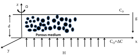
Figure 1.
Physical configuration.
Here, , , K, p, , , g, t, , , and are the acceleration coefficient, dynamic viscosity, permeability, dynamic pressure, reference density, solute expansion coefficient, gravity acceleration, time, porosity, solute diffusion coefficient, and reaction rate of the solute, respectively. The dimensionless quantities are given as follows:
as well as the non-dimensional quantities
where , , , , and are the Rayleigh number, Taylor number, Hartmann number, Damkohler number, and Vadasz number, respectively. The non-dimensional form of the governing Equations (1)–(3) and the corresponding boundary conditions (4) are given by
subject to the boundary conditions
2.2. Basic Flow
The basic stationary flow of Equations (7)–(10) is as follows:
2.3. Linear Stability Analysis
The perturbation of the basic state for the Equations (7)–(10) is
By substituting Equation (13) into Equations (7)–(10), one obtains
subject to the boundary conditions
By taking the third component of the curl of Equation (15) and curl of curl of Equation (15), one obtains
From Equations (16), (18) and (19), we obtain
where
Let us introduce the normal mode by writing that the perturbation is in the form of
where l and m are the wave numbers along x and y directions and is a complex parameter. Substituting Equation (24) into Equation (20), one obtains
where and .
2.4. Stationary Mode
To study the stationary stability, take in the Rayleigh number for the exchange of the stabilities at the onset of stationary convection, say . It is given as
The critical Rayleigh number at the onset of stationary convection is
The above stationary Rayleigh number reduces to with the critical values in the absence of a magnetic field, Coriolis effect, and chemical reaction effect, which agrees with the results of Horton and Rogers [41] and Lapwood [42] for the onset of convection in a porous layer.
2.5. Oscillatory Mode
To study the oscillatory stability, take . The Rayleigh number at the onset of oscillatory convection is
where
3. Artificial Neural Network Modeling
Let us now present some basis for the ANN modeling. An ANN is a computing system based on biological neural networks (which are interconnected) that resemble a brain. In general, ANN can be used to predict data. In this study, we used a network with three layers: input, hidden, and output, as well as other components, such as feed-forward propagation, an optimal number of neurons, and backpropagation (update weights and biases) (see Figure 2 and Figure 3). To train the suggested network, we use the Levenberg–Marquardt backpropagation algorithm, as proposed by Yu and Wilamowski [46]. To prepare the organization, data are first divided into three groups. A total of 650 datasets were utilized to train, test, and validate the ANN model, with 70%, 15%, and 15% of the data being randomly allocated for preparing and assessing. The optimal number of neurons () for the best performing artificial neural network architecture is determined by examining three different statistical values: coefficient of determination (), root mean square error (), and root mean relative error (), which are defined by
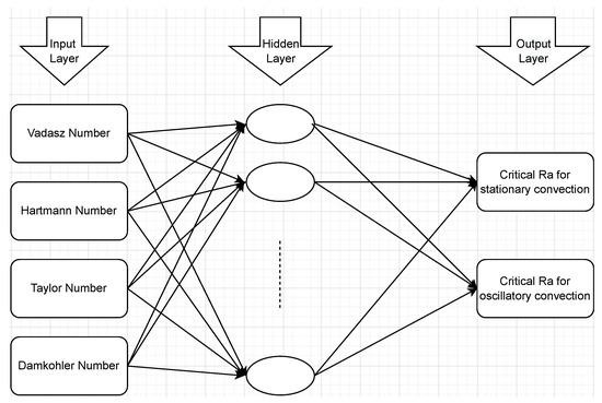
Figure 2.
Schematic representation of a multilayer feed-forward network consisting of two inputs, one hidden layer, and two outputs.
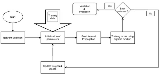
Figure 3.
Flow chart of the artificial neural network.
Here, is the simulated critical Rayleigh number, is the ANN critical Rayleigh number, the index i refers to the i-th experiment, bar denotes average value, and N is data size or number. See Seo et al. [45] for further details on these measures. The regression plots of training, testing, and validation for these three different sets are illustrated in Figure 4. The values of , , and for different values of , , , and are illustrated in Table 1 and Table 2. From these tables, it is clear that the present ANN model can predict the critical for linear stability analysis for different , , , and .
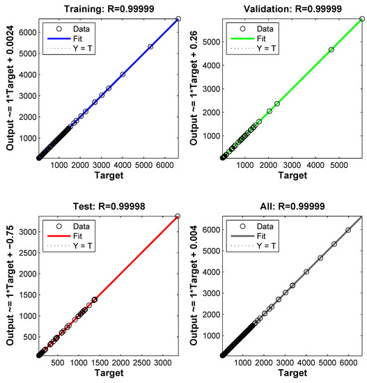
Figure 4.
Regression plots for training, validation, and testing; the targets are simulated data and the outputs are ANN-predicted data.

Table 1.
Calculated stationary values of , , and at various values of , , and .
Table 2.
Calculated oscillatory values of , , and at various values of , , and .
4. Discussion
The numerical results and discussion are presented in this section. In this results part, we evaluated a numerical study of the effect of the magnetic field and rotation on the onset of dissolution-driven convection saturated porous layer with ANN prediction. The critical Rayleigh number at the onset of stationary () and oscillatory () convection is obtained for the prescribed values of the other parameters. The investigations are performed for various values of the Hartmann number, Taylor number, Vadasz number, and Damkohler number. In Figure 5, Figure 6, Figure 7, Figure 8, Figure 9 and Figure 10, solid and dotted lines represent the stationary and oscillatory convection, respectively. The following physically realistic range of these parameters is considered: [37], [22], [40], and [23].
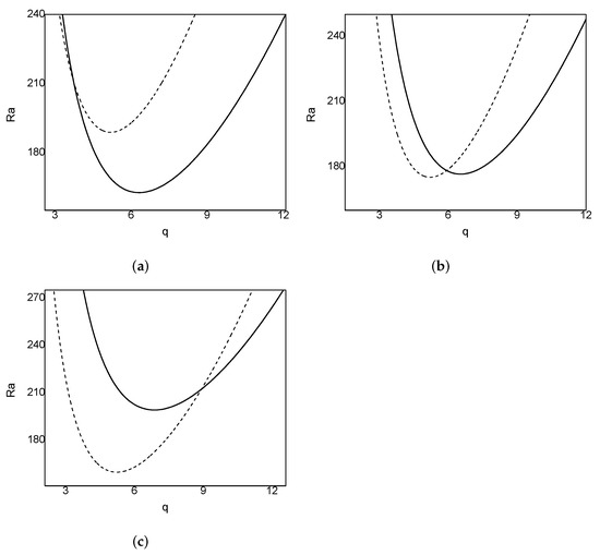
Figure 5.
Neutral curves (solid lines represent the stationary convection and dotted lines represent the oscillatory convection) for , , : (a) , (b) , (c) .
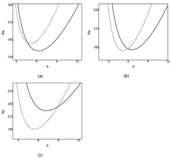
Figure 6.
Neutral curves (solid lines represent the stationary convection and dotted lines represent the oscillatory convection) for , , : (a) , (b) , (c) .
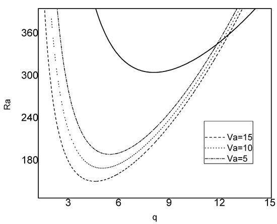
Figure 7.
Neutral curves (solid lines represent the stationary convection and dotted lines represent the oscillatory convection) for , , .
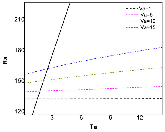
Figure 8.
Plots of the critical as the function of for .
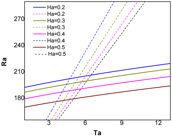
Figure 9.
Plots of critical as the function of for , .
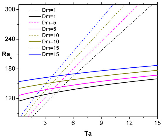
Figure 10.
Plots of critical as the function of for , .
First, we shall discuss the theory of bifurcation points in Figure 5, Figure 6 and Figure 7, the results obtained numerically by linear and weakly nonlinear stability analysis. Takens–Bogdanov and codimension two bifurcation points are identified in these figures. Takens–Bogdanov bifurcation point is the point at which the oscillatory neutral curve intersects the stationary neutral curve and approaches zero as the intersection point is approached. At the Takens–Bogdanov bifurcation point, we have
The codimension two bifurcation point is the intersection between a Hopf and Pitchfork bifurcation with distinct wave numbers. At the codimension two bifurcation point, we have
The effect of the Vadasz number on the neutral curves is presented in Figure 8. We find that the is independent of the Vadasz number , whereas the decreases with a decrease in the value of the Vadasz number . This reports the porosity effects on driven convection in a Newtonian-fluid-saturated porous layer. Furthermore, from this figure, one can notice that for , there exists a threshold such that for , stationary convection sets in, while for , there is a switch from stationary to oscillatory convection. Similar behavior can be observed for the other values of .
Figure 9 illustrates the effect of the magnetic field on the onset of convection. From this figure, one can observe that the Hartmann number has a stabilizing effect on stationary convection. On the contrary, the Hartmann number has a stabilizing effect on oscillatory convection. We find that the minimum value of the stationary Rayleigh number for stationary mode increases with increasing Hartmann number . On the other hand, the minimum value of the oscillatory Rayleigh number decreases with an increase in the value of the Hartmann number . Thus, has a contrasting effect on the stability of the system in the case of stationary and oscillatory modes. From this figure, we notice that for , there exists a threshold such that for , oscillatory convection sets in, while for , there is a switch from oscillatory to stationary convection. Similar behavior can be observed for the other values of .
Similarly, Figure 10 depicts the effect of on the system. From this figure, we see that the effect of increasing is to increase the and , implying that has a stabilizing effect on the onset of dissolution-driven convection in a porous medium. This can be explained as follows. An increase in the value of promotes the dissolution reaction to absorb some of the heat energy, causing the surrounding environment to feel cold. Hence, a larger solute gradient is required for the onset of convection so that the system is stabilized. We find that for fixed values of other physical parameters, there exists a critical Taylor number such that when , convection begins as an oscillatory type, and when , the convection switches to stationary. Further, when , the stationary and oscillatory modes occur simultaneously.
Furthermore, Figure 8, Figure 9 and Figure 10 demonstrate the Coriolis effect on the onset of convection. All of these figures show that the and increase as the Taylor number increases. Hence, the Taylor number has a stabilizing effect on the system. This can be explained as follows: in the fluid, the rotation creates vorticity. As a result, the fluid has a faster velocity in horizontal planes. Hence, the perpendicular velocity of the fluid decreases. Therefore, the convection does not start right away.
The comparison of numerical and predicted ANN data of the critical with different values of , , , and is shown in Figure 11 and Figure 12. From all these figures, it is obvious to see that the trained predictive ANN model holds well with the numerical results.
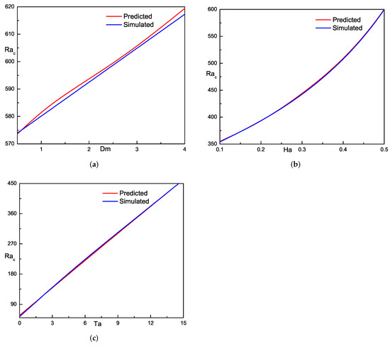
Figure 11.
Comparison of the simulated and ANN-predicted critical Rayleigh number values for (a) , (b) , and (c) .
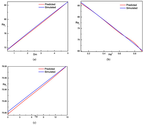
Figure 12.
Comparison of the simulated and ANN-predicted critical Rayleigh number values for (a) , (b) , and (c) .
5. Conclusions
In the present analysis, the onset of dissolution-driven convection in a porous layer with the effect of the magnetic field and rotation is studied. The behavior of various physical parameters is investigated. The results can be summarized as follows: Takens–Bogdanov and codimension two bifurcation points are identified. The Vadasz number does not show any effect on stationary convection, whereas it has a destabilizing effect on oscillatory convection. The Hartmann number has destabilizing and stabilizing effects on stationary and oscillatory convection, respectively. The Damkohler number has a stabilizing effect on the system. Furthermore, an artificial neural network (ANN) is used to model and predict the critical Rayleigh numbers. The simulated and predicted values of the proposed ANN model were found to be highly close, indicating that the expected critical Rayleigh number and the observed critical Rayleigh number are quite similar.
In future work, we plan to study linear instability and nonlinear stability. Another interesting problem is to investigate the stationary or oscillatory convection at the onset of instability using Brinkmann’s law.
Author Contributions
Conceptualization, G.S.K.R. and N.V.K.; methodology, G.S.K.R., N.V.K., R.R., K.K.P. and C.C.; software, G.S.K.R., N.V.K., R.R., K.K.P. and C.C.; validation, G.S.K.R., N.V.K., R.R., K.K.P. and C.C.; formal analysis, G.S.K.R., N.V.K., R.R., K.K.P. and C.C.; investigation, G.S.K.R., N.V.K., R.R., K.K.P. and C.C.; resources, G.S.K.R., N.V.K., R.R., K.K.P. and C.C.; data curation, G.S.K.R., N.V.K., R.R., K.K.P. and C.C.; writing—original draft preparation, G.S.K.R., N.V.K., R.R., K.K.P. and C.C.; writing—review and editing, G.S.K.R., N.V.K., R.R., K.K.P. and C.C.; visualization, G.S.K.R., N.V.K., R.R., K.K.P. and C.C. All authors have read and agreed to the published version of the manuscript.
Funding
This research received no external funding.
Conflicts of Interest
The authors declare no conflict of interest.
References
- Ghoshal, P.; Kim, M.C.; Cardoso, S.S. Reactive–convective dissolution in a porous medium: The storage of carbon dioxide in saline aquifers. Phys. Chem. Chem. Phys. 2017, 19, 644–655. [Google Scholar] [CrossRef] [PubMed]
- Ilya, A.; Ashraf, M.; Ali, A.; Shah, Z.; Kumam, P.; Thounthong, P. Heat source and sink effects on periodic mixed convection flow along the electrically conducting cone inserted in porous medium. PLoS ONE 2021, 16, e0260845. [Google Scholar] [CrossRef] [PubMed]
- Alshehri, A.; Shah, Z. Computational analysis of viscous dissipation and Darcy-Forchheimer porous medium on radioactive hybrid nanofluid. Case Stud. Therm. Eng. 2022, 30, 101728. [Google Scholar] [CrossRef]
- Vo, D.D.; Shah, Z.; Sheikholeslami, M.; Shafee, A.; Nguyen, T.K. Numerical investigation of MHD nanomaterial convective migration and heat transfer within a sinusoidal porous cavity. Phys. Scr. 2019, 94, 115225. [Google Scholar] [CrossRef]
- Jamshed, W.; Şirin, C.; Selimefendigil, F.; Shamshuddin, M.D.; Altowairqi, Y.; Eid, M.R. Thermal Characterization of Coolant Maxwell Type Nanofluid Flowing in Parabolic Trough Solar Collector (PTSC) Used Inside Solar Powered Ship Application. Coatings 2021, 11, 1552. [Google Scholar] [CrossRef]
- Mahabaleshwar, U.S.; Rekha, M.B.; Kumar, P.N.V.; Selimefendigil, F.; Sakanaka, P.H.; Lorenzini, G.; Nayakar, S.N.R. Mass transfer characteristics of MHD casson fluid flow past stretching/shrinking sheet. J. Eng. Thermophys. 2020, 29, 285–302. [Google Scholar] [CrossRef]
- Steinberg, V.; Brand, H. Convective instabilities of binary mixtures with fast chemical reaction in a porous medium. J. Chem. Phys. 1983, 78, 2655–2660. [Google Scholar] [CrossRef]
- Steinberg, V.; Brand, H.R. Amplitude equations for the onset of convection in a reactive mixture in a porous medium. J. Chem. Phys. 1984, 80, 431–435. [Google Scholar] [CrossRef]
- Gatica, J.E.; Viljoen, H.J.; Hlavacek, V. Interaction between chemical reaction and natural convection in porous media. Chem. Eng. Sci. 1989, 44, 1853–1870. [Google Scholar] [CrossRef]
- Pritchard, D.; Richardson, C.N. The effect of temperature-dependent solubility on the onset of thermosolutal convection in a horizontal porous layer. J. Fluid Mech. 2007, 571, 59–95. [Google Scholar] [CrossRef]
- Rees, D.A.S.; Selim, A.; Ennis-King, J. The Instability of Unsteady Boundary Layers in Porous Media; Springer: Berlin/Heidelberg, Germany, 2008. [Google Scholar]
- Slim, A.C.; Ramakrishnan, T. Onset and cessation of time-dependent, dissolution-driven convection in porous media. Phys. Fluids 2010, 22, 124103. [Google Scholar] [CrossRef]
- Bestehorn, M.; Firoozabadi, A. Effect of fluctuations on the onset of density-driven convection in porous media. Phys. Fluids 2012, 24, 114102. [Google Scholar] [CrossRef]
- Kim, M.C.; Choi, C.K. Effect of first-order chemical reaction on gravitational instability in a porous medium. Phys. Rev. E 2014, 90, 053016. [Google Scholar] [CrossRef] [PubMed]
- Hill, A.A.; Morad, M.R. Convective stability of carbon sequestration in anisotropic porous media. Proc. R. Soc. Math. Phys. Eng. Sci. 2014, 470, 20140373. [Google Scholar] [CrossRef]
- Al-Sulaimi, B. The energy stability of Darcy thermosolutal convection with reaction. Int. J. Heat Mass Transf. 2015, 86, 369–376. [Google Scholar] [CrossRef]
- Emami-Meybodi, H. Stability analysis of dissolution-driven convection in porous media. Phys. Fluids 2017, 29, 014102. [Google Scholar] [CrossRef]
- Salibindla, A.K.; Subedi, R.; Shen, V.C.; Masuk, A.U.; Ni, R. Dissolution-driven convection in a heterogeneous porous medium. J. Fluid Mech. 2018, 857, 61–79. [Google Scholar] [CrossRef]
- Gautam, K.; Narayana, P.A.L. On the stability of carbon sequestration in an anisotropic horizontal porous layer with a first-order chemical reaction. Proc. R. Soc. A 2019, 475, 20180365. [Google Scholar] [CrossRef]
- Babu, A.B.; Koteswararao, N.V.; Reddy, G.S. Instability conditions in a porous medium due to horizontal magnetic field. In Numerical Heat Transfer and Fluid Flow; Springer: Singapore, 2019; pp. 621–628. [Google Scholar]
- Babu, A.B.; Rao, N.; Tagare, S.G. Weakly nonlinear thermohaline convection in a sparsely packed porous medium due to horizontal magnetic field. Eur. Phys. J. Plus 2021, 136, 795. [Google Scholar] [CrossRef]
- Babu, A.B.; Anilkumar, D.; Rao, N.V.K. Weakly nonlinear thermohaline rotating convection in a sparsely packed porous medium. Int. J. Heat Mass Transf. 2022, 188, 122602. [Google Scholar] [CrossRef]
- Reddy, G.S.K.; Ragoju, R. Thermal instability of a Maxwell fluid saturated porous layer with chemical reaction. Spec. Top. Rev. Porous Media Int. J. 2022, 13, 33–47. [Google Scholar] [CrossRef]
- Yin, Y.; Qu, Z.; Zhu, C.; Zhang, J. Visualizing gas diffusion behaviors in three-dimensional nanoporous media. Energy Fuels 2021, 35, 2075–2086. [Google Scholar] [CrossRef]
- Yin, Y.; Qu, Z.; Prodanović, M.; Landry, C.J. Identifying the dominant transport mechanism in single nanoscale pores and 3D nanoporous media. Fundam. Res. 2022. [Google Scholar] [CrossRef]
- Utech, H.P.; Flemmings, M.C. Elimination of solute banding in indium antimonide crystals by growth in a magnetic field. J. Appl. Phys. 1966, 37, 2021–2024. [Google Scholar] [CrossRef]
- Vives, C.; Perry, C. Effects of magnetically damped convection during the controlled solidification of metals and alloys. Int. J. Heat Mass Transf. 1987, 30, 479–496. [Google Scholar] [CrossRef]
- Garandet, J.P.; Alboussiere, T.; Moreau, R. Buoyancy driven convection in a rectangular enclosure with a transverse magnetic field. Int. J. Heat Mass Transf. 1992, 35, 741–748. [Google Scholar] [CrossRef]
- Alboussiere, T.; Garandet, J.P. Buoyancy-driven convection with a uniform magnetic field. Part 1. Asymptotic analysis. J. Fluid Mech. 1993, 253, 545–563. [Google Scholar] [CrossRef]
- Rudraiah, N.; Venkatachalappa, M.; Subbaraya, C.K. Combined surface tension and buoyancy-driven convection in a rectangular open cavity in the presence of a magnetic field. Int. J. Non-Linear Mech. 1995, 30, 759–770. [Google Scholar] [CrossRef]
- Davoust, L.; Cowley, M.D.; Moreau, R.; Bolcato, R. Buoyancy-driven convection with a uniform magnetic field. Part 2. Experimental investigation. J. Fluid Mech. 1999, 400, 59–90. [Google Scholar] [CrossRef]
- Priede, J.; Gerbeth, G. Hydrothermal wave instability of thermocapillary-driven convection in a transverse magnetic field. J. Fluid Mech. 2000, 404, 211–250. [Google Scholar] [CrossRef]
- Pirmohammadi, M.; Ghassemi, M.; Sheikhzadeh, G.A. The effect of a magnetic field on buoyancy-driven convection in differentially heated square cavity. In Proceedings of the 2008 14th Symposium on Electromagnetic Launch Technology, Victoria, BC, Canada, 10–13 June 2008; pp. 1–6. [Google Scholar]
- Sankar, M.; Venkatachalappa, M.; Do, Y. Effect of magnetic field on the buoyancy and thermocapillary driven convection of an electrically conducting fluid in an annular enclosure. Int. J. Heat Fluid Flow 2011, 32, 402–412. [Google Scholar] [CrossRef]
- Erglis, K.; Tatulcenkov, A.; Kitenbergs, G.; Petrichenko, O.; Ergin, F.G.; Watz, B.B.; Cbers, A. Magnetic field driven micro-convection in the Hele–Shaw cell. J. Fluid Mech. 2013, 714, 612–633. [Google Scholar] [CrossRef]
- Babu, A.B.; Reddy, G.S.K.; Tagare, S.G. Nonlinear magneto convection due to horizontal magnetic field and vertical axis of rotation due to thermal and compositional buoyancy. Results Phys. 2019, 12, 2078–2090. [Google Scholar] [CrossRef]
- Govender, S.; Vadasz, P. The effect of mechanical and thermal anisotropy on the stability of gravity driven convection in rotating porous media in the presence of thermal non-equilibrium. Transp. Porous Media 2007, 69, 55–66. [Google Scholar] [CrossRef]
- Babu, A.B.; Reddy, G.S.K.; Tagare, S.G. Nonlinear magnetoconvection in a rotating fluid due to thermal and compositional buoyancy with anisotropic diffusivities. Heat Transf. Asian Res. 2020, 49, 335–355. [Google Scholar] [CrossRef]
- Wang, S.; Wenchang, T. The onset of Darcy–Brinkman thermosolutal convection in a horizontal porous media. Phys. Lett. A 2009, 373, 776–780. [Google Scholar] [CrossRef]
- Deepika, N.; Murthy, P.V.S.N.; Narayana, P.A.L. The effect of magnetic field on the stability of double-diffusive convection in a porous layer with horizontal mass throughflow. Transp. Porous Media 2020, 134, 435–452. [Google Scholar] [CrossRef]
- Horton, C.W.; Rogers, F.T. Convection currents in a porous medium. J. Appl. Phys. 1945, 16, 367–370. [Google Scholar] [CrossRef]
- Lapwood, E.R. Convection of a fluid in a porous medium. Math. Proc. Camb. Philos. Soc. 1948, 44, 508–521. [Google Scholar] [CrossRef]
- Dey, P.; Abhijit, S.; Das, A.K. Development of GEP and ANN model to predict the unsteady forced convection over a cylinder. Neural Comput. Appl. 2016, 27, 2537–2549. [Google Scholar] [CrossRef]
- Rana, P.; Gupta, V.; Kumar, L. LTNE magneto-thermal stability analysis on rough surfaces utilizing hybrid nanoparticles and heat source with artificial neural network prediction. Appl. Nanosci. 2021. [Google Scholar] [CrossRef]
- Seo, Y.M.; Pandey, S.; Lee, H.U.; Choi, C.; Park, Y.G.; Ha, M.Y. Prediction of heat transfer distribution induced by the variation in vertical location of circular cylinder on Rayleigh-Bénard convection using artificial neural network. Int. J. Mech. Sci. 2021, 209, 106701. [Google Scholar] [CrossRef]
- Yu, H.; Wilamowski, B.M. Levenberg–Marquardt training. In Intelligent Systems; CRC Press: Boca Raton, FL, USA, 2018; Chapter 12; pp. 1–16. [Google Scholar]
- Seo, Y.M.; Luo, K.; Ha, M.Y.; Park, Y.G. Direct numerical simulation and artificial neural network modeling of heat transfer characteristics on natural convection with a sinusoidal cylinder in a long rectangular enclosure. Int. J. Heat Mass Transf. 2020, 152, 119564. [Google Scholar] [CrossRef]
- Khosravi, R.; Rabiei, S.; Bahiraei, M.; Teymourtash, A.R. Predicting entropy generation of a hybrid nanofluid containing graphene–platinum nanoparticles through a microchannel liquid block using neural networks. Int. Commun. Heat Mass Transf. 2019, 109, 104351. [Google Scholar] [CrossRef]
- Amani, M.; Amani, P.; Bahiraei, M.; Wongwises, S. Prediction of hydrothermal behavior of a non-Newtonian nanofluid in a square channel by modeling of thermophysical properties using neural network. J. Therm. Anal. Calorim. 2019, 135, 901–910. [Google Scholar] [CrossRef]
- Bahiraei, M.; Heshmatian, S.; Keshavarzi, M. Multi-criterion optimization of thermohydraulic performance of a mini pin fin heat sink operated with ecofriendly graphene nanoplatelets nanofluid considering geometrical characteristics. J. Mol. Liq. 2019, 276, 653–666. [Google Scholar] [CrossRef]
- Bahiraei, M.; Mazaheri, N.; Hosseini, S. Neural network modeling of thermo-hydraulic attributes and entropy generation of an ecofriendly nanofluid flow inside tubes equipped with novel rotary coaxial double-twisted tape. Powder Technol. 2020, 369, 162–175. [Google Scholar] [CrossRef]


Publisher’s Note: MDPI stays neutral with regard to jurisdictional claims in published maps and institutional affiliations. |
© 2022 by the authors. Licensee MDPI, Basel, Switzerland. This article is an open access article distributed under the terms and conditions of the Creative Commons Attribution (CC BY) license (https://creativecommons.org/licenses/by/4.0/).