Abstract
Multi-objective evolutionary algorithms (MOEAs) have been successfully applied for the numerical treatment of multi-objective optimization problems (MOP) during the last three decades. One important task within MOEAs is the archiving (or selection) of the computed candidate solutions, since one can expect that an MOP has infinitely many solutions. We present and analyze in this work ArchiveUpdateHD, which is a bounded archiver that aims for Hausdorff approximations of the Pareto front. We show that the sequence of archives generated by ArchiveUpdateHD yields under certain (mild) assumptions with a probability of one after finitely many steps a -approximation of the Pareto front, where the value is computed by the archiver within the run of the algorithm without any prior knowledge of the Pareto front. The knowledge of this value is of great importance for the decision maker, since it is a measure for the “completeness” of the Pareto front approximation. Numerical results on several well-known academic test problems as well as the usage of ArchiveUpdateHD as an external archiver within three state-of-the-art MOEAs indicate the benefit of the novel strategy.
1. Introduction
This work is dedicated to the 60th birthday of Professor Kalyanmoy Deb, a pioneer and highly impactful and influential proponent of Evolutionary Multi-Objective Optimization (EMO) for the last three decades. In particular, the seminal work Combining Convergence and Diversity in Evolutionary Multiobjective Optimization by Marco Laummans, Lothar Thiele, Kalyanmoy Deb, and Eckart Zitzler [1] has been a motivation of the second author to consider the challenging and fruitful field of archiving in EMO.
Multi-objective optimization problems (MOPs), i.e., problems where several conflicting objectives have to be optimized concurrently, naturally arise in many real-world applications (e.g., [2,3,4,5,6,7,8]). While one can expect one optimal solution if “only” one objective is being considered, the solution set of an MOP (the so-called Pareto set, respectively, its image, the Pareto front) typically forms at least locally a manifold of a certain dimension [9]. One important task in multi-objective optimization (MOO) is hence to identify a “suitable” finite size approximation of these solution sets. Multi-objective evolutionary algorithms (MOEAs) represent an important class of algorithms for the numerical treatment of such problems. MOEAs have caught the interest of researchers and practitioners due to their global nature and robustness and since they require only minimal assumptions on the model (e.g., [2,10]). The process to elect a subset of the candidate solutions generated by the MOEA is called selection or archiving. Existing archiving/selection strategies can be roughly divided into two classes (see subsequent section for more details): (i) mechanisms that maintain sets those cardinalities are equal or do not exceed a certain pre-defined cardinality—which we will call bounded archivers in the following—and (ii) archivers that are based on the concept of -dominance. Such archivers generate sequences of archives with monotonic behavior, i.e., no deterioration of cyclic behavior can be observed during the run of an algorithm. Furthermore, for , these archives yield certain limit approximation qualities that can be adjusted a priori, mainly by choosing the values of which comes rather naturally at least if the MOP arises from a real-world application. On the other hand, the magnitudes of the final archives are entirely determined by and some other design parameters, which are set a priori and are supposed to remain fixed during the computation, and the size of the Pareto front, which is a priori of course unknown. It has turned out that most EMO researchers prefer to have a fixed number of elements in the archives, e.g., for the sake of a better comparison to other methods but also to avoid the necessity of storing an unexpected large amount of candidate solutions. The latter problem is apparently by construction not given by bounded archives. For most strategies from class (i), however, no theoretical analyses such as convergence properties are known. For many distance-based methods, it is further known that cyclic behavior and deterioration can occur during the run of the algorithm. It is hence fair to say that these methods do not tap the full potential, since any MOEA using such a strategy will not converge regardless of the regions they explore during the run of the algorithm. An exception is the bounded archive proposed in [11], which yields under certain (mild) assumptions and with the probability of one -Pareto set in the limit, where is the smallest possible value with respect to to the bound of the archives.
In this paper, we propose a bounded archiver that is based on distance, dominance and -dominance that offers quasi-monotonic behavior and yields approximation qualities in the limit. More precisely, ArchiveUpdateHD aims for Hausdorff approximations of the Pareto front (i.e., evenly spread solutions along the Pareto front). Under certain (mild) assumptions on the generation process, it will be shown that the Hausdorff distances of the images of the archives and the Pareto front are bounded by a value , which is computed by the archiver during the run of the algorithm. Numerical experiments show that this value indeed represents a good approximation of the actual Hausdorff distance (while a better strategy is proposed for bi-objective problems). During the run of the algorithm, two design parameters are adjusted adaptively during the run of the algorithm (one being the value of for the -dominance). Since these values will become stationary during the search process, one can expect monotonic behavior from a certain stage of the search process. The knowledge of the Hausdorff distance of and is important information for the decision maker (DM), since it represents the maximal error in the approximation. If not needed (i.e., depending on the chosen initial design parameters), the magnitudes of the archivers will not reach the pre-defined size N. Else, the value computed by the archiver is an important piece of information, since it tells the DM if the approximation is “complete enough” or not. In the latter case, the computation may have to be repeated using an increased value of N. A preliminary version of this work can be found in [12], which is restricted to bi-objective problems and contains fewer empirical results.
The rest of this document is structured as follows: Section 2 briefly summarizes the background that is required for the understanding of the sequel and presents the related work. In Section 3, the new archiver ArchiveUpdateHD is discussed and analyzed, first for bi-objective problems and after that for the general number of objectives. In Section 4, some numerical results and comparisons are presented and discussed. Finally, in Section 5, conclusions are drawn, and possible paths for future research are mentioned.
2. Background and Related Work
Here, we consider continuous multi-objective optimization problems (MOPs) that can be expressed as follows:
The map F is defined by the individual objective functions , i.e.,
where each , , is assumed to be continuous. We stress, however, that the archiver presented below can also be applied to discrete problems. Q is the domain or feasible set of the problem, which is typically expressed by equality and inequality constraints. We assume Q to be compact (i.e., closed and bounded). If objectives are considered, the problem is also termed a bi-objective problem (BOP).
In order to define optimality in multi-objective opimization, the concept of dominance can be used: for two vectors we say that x is less than y () if , , analogously for the relation . We say that is dominated by () with respect to (MOP) if and , else we say that y is non-dominated by x. Finally, is called Pareto optimal or simply optimal with respect to (MOP) if there exists no that dominates x. The Pareto set is the set of all optimal solutions with respect to (MOP), and its image is called the Pareto front. One can expect that both the Pareto set and Pareto front are from at least locally objects of dimension , where k is the number of objectives considered in the MOP [9].
For the convergence analysis, we will consider a very general class of algorithms, called Generic Stochastic Search Algorithm (GSSA), first considered by Laumanns et al. [1]. An algorithm of this class consists of a process to generate new candiate solutions together with an update strategy. Algorithm 1 shows the pseudocode of GSSA.
| Algorithm 1 Generic Stochastic Search Algorithm |
| 1: drawn at random |
| 2: |
| 3: fordo |
| 4: |
| 5: |
| 6:end for |
In the following, we define the Hausdorff distance and the averaged Hausdorff distance , which we will use to assess the approximation qualities of the obtained Pareto front approximations (toward the actual Pareto fronts).
Definition 1.
Let and . The semi-distance and the Hausdorff distance are defined as follows:
- (a)
- (b)
- (c)
Definition 2
([13]). Let be finite sets. The value
where
and , is called the averaged Hausdorff distance between A and B.
We further define some objects that specify certain approximation qualities of Pareto front approximations. All of these objects are based on the concept of -dominance, which we will define first.
Definition 3
(-dominance). Let and . x is said to ϵ-dominate y (in short: ) with respect to (MOP) if
Definition 4
(-(approximate) Pareto front, [1]). Let and .
Definition 5
(-tight -(approximate) Pareto front, [14]). Let and .
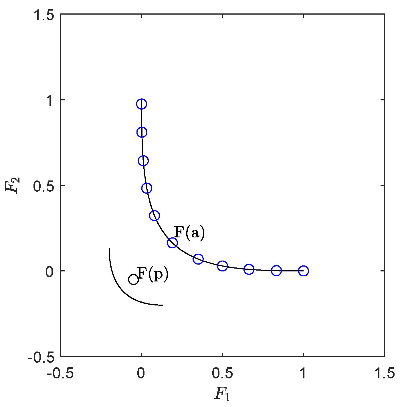
The archiver we propose in this work, ArchiveUpdateHD, aims for -tight -Pareto fronts for particular values of and . The sole usage of -dominance for the Pareto front approximations may lead to gaps in particular when parts of the front are flat. The -tight -(approximate) Pareto fronts also take into account the distance of the Pareto front toward the candidate set, leading to better approximations in the Hausdorff sense (see Figure 1).
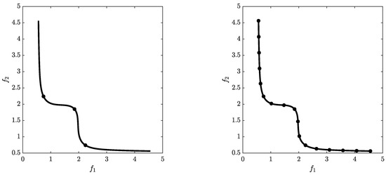
Figure 1.
Gaps in the approximation can occur when -dominance is used exclusively in the selection/archiving of the candidate solutions (left). -tight -(approximate) Pareto fronts also consider the distance of the Pareto front toward the archive (right).
Since one can expect infinitely many solutions for a continuous MOP, it is inevitable in (continuous) evolutionary multi-objective optimization (EMO) that not all promising solutions can be kept during the run of an algorithm. Instead, one has to elect a subset of candiate solutions in each iteration so that this sequence eventually leads to a “suitable” representation of the Pareto set/front of the given problem. This process is typically called “selection” within MOEAs and “archiving” if an external set of candidate solutions (archive) is maintained during the run of a MOEA (though of course both terms can be used interchangeably).
Three main classes of MOEAs exist: (a) dominance-based [15,16,17,18], (b) decomposition-based [19,20,21,22,23,24,25], and (c) indicator-based [26,27,28,29,30] algorithms. The selection strategies for MOEAs of class (b) or (c) are rather straightforward: the selection in a decomposition-based MOEA is done implicitly by the chosen scalarizing functions, and the selection in an indicator-based MOEA is typically handled via considering the indicator contributions. These two approaches come on the one hand with a monotonic behavior of the sequence of approximations (i.e., no deterioration can occur). On the other hand, these selection strategies do not guarantee convergence toward the best approximation (e.g., [29,31]). The selection of the first dominance-based MOEAs is based on non-dominated sorting in combination with niching techniques (e.g., [32,33,34]). Due to missing elite preservation, none of these methods converge in the mathematical sense. Later MOEAs such as SPEA [35], PAES [18], SPEA-II [16], and NSGA-II [15] include such elite preservation leading to much better overall performance. However, also for these algorithms, no convergence properties (again, in the mathematical sense) are known. Rudolph [36,37,38,39] and Hanne [40,41,42,43] have studied convergence properties of MOEA frameworks. These studies are mainly concerned with the convergence of individuals of the populations toward the Pareto set/front, while the magnitudes and the distributions of the resulting populations are not considered.
Archiving strategies with bounded archive size based on adaptive grid selection have been considered in [44,45,46]. Bounded archivers in particular for hypervolume approximations have been proposed in [47,48]. Both archivers yield monotonic behavior in the approximation qualities of the obtained sequence of archives.
Laumanns et al. considered the class of algorithms GSSA as described above [1,49] which allows to focus on the archiver under certain (mild) assumptions on the generator. In both studies, archivers were considered, aiming for several approximations of the Pareto front, where finitely many iterations were considered. Later, further archivers have been proposed based on -dominance using the framework of GSSA to perform convergence analysis [14,50,51,52,53,54].
In [11], Laumanns and Zenklusen propose two bounded archivers that use adaptive schemes to obtain approximations of the Pareto front. Another adaptive archiving strategy is proposed in [55] that utilizes a particular discretization of the objective space of the given problem. A strategy that is based on the convex hull of individual minima in order to increase diversity of the solutions is proposed in [56].
Recently, the use of external archives has become more popular [57,58,59,60,61,62] in particular for the treatment of real-world applications where function evaluations are expensive, and where it is hence advisable to maintain all promising candidate solutions. Consequently, most of these archivers are unbounded [63,64,65,66,67]. For the treatment of in particular MOPs with many objectives—also called many objective problems—MOEAs have been proposed that utilize two archives, one aiming for convergence and one aiming for diversity [68,69].
3. ArchiveUpdateHD
We will in this section propose and discuss the novel archiver ArchiveUpdateHD. Since the considerations of the distances as well as the Hausdorff approximations can be done more accurately for —where we can assume the Pareto front to locally form a curve, and hence, the elements of the approximations can be arranged via a sorting in objective space—we first address the bi-objective case and will afterwards consider the archiver for problems with .
3.1. The Bi-Objective Case
The pseudocode of ArchiveUpdateHD for bi-objective problems is shown in Algorithm 2. This archiver aims for approximations of the Pareto front of a given BOP in the Hausdorff sense (i.e., for solutions that are evenly spread along the Pareto front). The archiver is based (i) on the distances among the candidate solutions (lines 18–36 of Algorithm 2), (ii) “classical” dominance or elite preservation (lines 5 and 9) as well as (iii) the concept of -dominance (line 5). The archiver can roughly be divided into two parts: an acceptance strategy to decide if an incoming candidate solution p should be considered (line 5), and a pruning technique (mainly lines 18–36, but also lines 11–14) which is applied if the size of the archive has exceeded a predefined budget N of archive entries.
In the following, we will describe ArchiveUpdateHD as in Algorithm 2 in more detail. This algorithm contains several elements that have to be incorporated in order to guarantee convergence. After the convergence analysis (Theorem 1), we will discuss more practical realizations of the algorithm.
In line 5, it is decided if a candidate solution p should be (at least temporarily) added to the existing archive A. This is the case if (a) none of the entries -dominates p ( being a safety factor needed to guarantee convergence, see below for practical realizations), or if (b) none of the entries dominates p and for none of the entries the distance is less or equal than . Throughout this work, denotes the Euclidean norm. We stress that this acceptance strategy is identical to the one of the archiver ArchiveUpdateTight2 [14], which we will need for the upcoming convergence analysis.
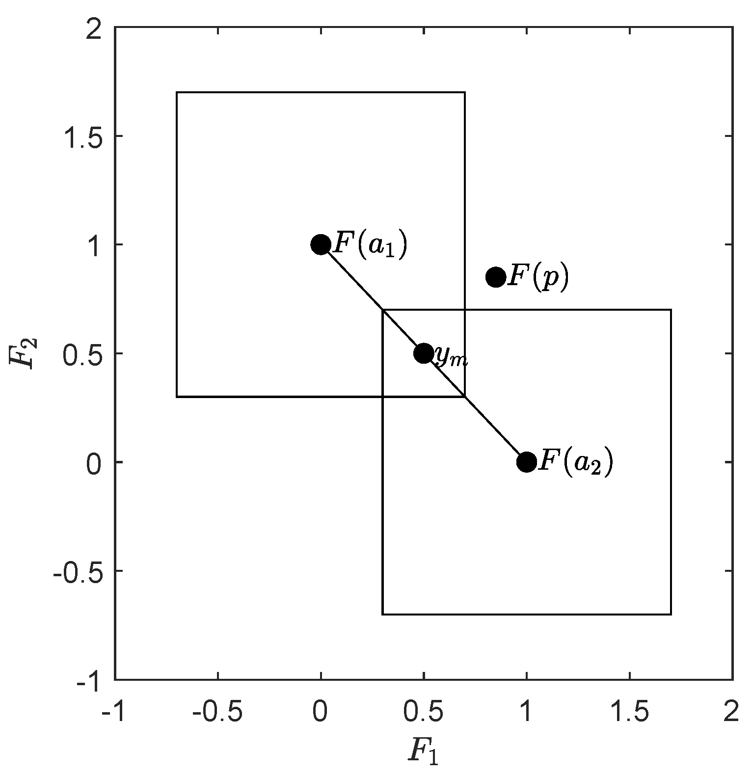
If the candidate solution p is accepted, it will be added to A. Next, all other entries dominated by p will be discarded (lines 8–10). Hence, all archives generated by ArchiveUpdateHD only contain mutually non-dominated elements (elite preservation). If the distance is larger than for any of these dominated archive entries a, a “reset” is executed for and : is set to (where another safety factor). Next, and are updated using this new minimal value. The idea behind this reset is as follows: if and the distance of and is larger than , then p and a could be located in different connected components of the set of (local) solutions of the bi-objective problem. Since the values both of and are determined by the length of the (known) Pareto front, their values have to be set back, since a “jump” to a new connected component may lead to a new length. See Figure 2 for a hypothetical scenario. The value of has to be (slightly) increased in each reset in order to avoid the possible of a cyclic behavior in the sequence of archives (which, in fact, has not been observed in our computations).

Figure 2.
A hypothetical scenario that can happen for multi-modal problems: first, a front that is only locally optimal is detected by the search process and approximated by the archiver. If later, a candidate p is computed such that lies on a “better” front, the current values of and may not be adequate any more to suitably approximate this front.
If exceeds the predefined magnitude N, it is decided in lines 18–36 which of the elements of A has to be discarded (pruning). For objectives, we can order all the entries of the archives (e.g., as done here: in ascending order wrt objective ). Then, the vector of distances can be simply computed via:
For an index m chosen from , either or is then removed from A, which is done in lines 23–33. The aim of ArchiveUpdateHD is to maintain good approximations of the end points of the Pareto front. Accordingly, , respectively, , are always discarded instead of and , respectively (lines 23–26). The rationale behind the selection in lines 28–33 is to keep the archive of size N with the most evenly distributed elements.
| Algorithm 2 ArchiveUpdateHD |
| Require: Problem (MOP), where , P: current population, : current archive, : current value of , : minimal value of , , : safety factors, N: upper bound for archive size |
| Ensure: updated archive A, updated values for , , and |
| 1: |
| 2: |
| 3: |
| 4: for all do |
| 5: if then |
| 6: |
| 7: end if |
| 8: for all do |
| 9: if then |
| 10: |
| 11: if then ▹ reset and |
| 12: |
| 13: |
| 14: |
| 15: end if |
| 16: end if |
| 17: end for |
| 18: if then ▹ apply pruning |
| 19: |
| 20: |
| 21: sort A (e.g., according to ) |
| 22: compute as in (8) |
| 23: choose |
| 24: if then |
| 25: ▹ remove 2nd entry |
| 26: else if then |
| 27: ▹ remove 2nd but last entry |
| 28: else |
| 29: |
| 30: |
| 31: if then |
| 32: |
| 33: else |
| 34: |
| 35: end if |
| 36: end if |
| 37: end if |
| 38:end for |
| 39:return |
In the following, we investigate the limit behavior of ArchiveUpdateHD.
Theorem 1.
Let (MOP) be given and be compact, and let there be no weak Pareto points in . Furthermore, let F be continuous and injective, and
Then, an application of Algorithm 1, where ArchiveUpdateHD (Algorithm 2) is used to update the archive, leads to a sequence of archives , where the following holds:
- (a)
- There exists a and such that
- (b)
- There exists with probability one a such that is a -tight ϵ-approximate Pareto front with respect to (MOP) for all , where .
- (c)
- (d)
- There exists a such that
Proof.
We first show that during the run of the algorithm, only finitely many changes of the value of (and hence also of ) can occur. Since F is continuous and the domain is compact, also the image is compact, and hence, in particular bounded. ArchiveUpdateHD changes the value of in two cases: if (i) a reset of and is executed (line 12) or if (ii) the pruning technique is applied (line 19). In case of (i), the value of is increased by a constant factor . The value of after the i-th reset is hence equal to or larger than , where denotes the value of at the start of the algorithm. A reset is applied if the distance of the image of the candidate solution p to the image of an archive element a is larger than the current value of (line 11). Since is bounded, only a finite number of such resets can be applied during the run of the algorithm.
Case (ii) happens if the magnitude of the current archive is . New candidate solutions p are added to the archive in lines 5 and 6 and lines 9 and 10. Lines 9 and 10 describe a dominance replacement which does not increase the magnitude of the archive. Hence, such replacements do not lead to an application of the pruning. A candidate p can be further added to the current archive A if one of the following statements is true (line 5):
Since is bounded, there exists for every a (large enough) so that , where . Similarly, if is large enough. Since in each pruning step, the value of is increased by the factor of and since only finitely many resets are executed, also only finitely many prunings can be applied during the run of the algorithm.
Note that ArchiveUpdateHD differs from ArchiveUpdateTight2 in two parts: the reset strategy (lines 11–15) and the pruning technique (lines 18–37), and that both these parts come with a change of the values of and . In other words, ArchiveUpdateHD is identical to ArchiveUpdateTight2 as long as no change in and occurs. For this case, we can hence apply the theoretical results on ArchiveUpdateTight2 for ArchiveUpdateHD. Now, consider a fixed value of (and hence also ). During the run, it can either be the case that (i) all magnitudes of are less than or equal to N (i.e., no pruning is applied), or that (ii) this magnitude is at one point, leading to an application of the pruning technique. In case (i), we can use Theorem 7.4 of [54] on ArchiveUpdateTight2: there exists with probability of one a such that the sets form a -tight -approximate Pareto front for all . Note that once forms such an object, no more resets can occur: assume there exists a candidate solution p that dominates an element , and where . The latter means that
which in turn means that a does not -approximate p, which is a contradiction to the assumption on . In case of (ii), the value of is simply not large enough for the N-element archive to form a -tight - approximate Pareto front. Again, by Theorem 7.4 of [54], there exists in this case with a probability of one a finite iteration number where the magnitude will exceed N. As discussed above, the pruning can only be applied finitely many times during the run of the algorithm. Hence, the value of will, with a probability of one, stay fixed from one iteration onwards, which proves part (a).
Parts (b) and (c) follow from Theorem 7.4 of [54] and part (a), and finally, part (d) follows from parts (b) and (c) and the definition of the Hausdorff distance. □
Remark 1.
- (a)
- Equation (9) is an assumption that has to be made on the generation process. It means that every neighborhood of every feasible point will be “visited” with probability one by after finitely many steps. For MOEAs, this, e.g., ensured if Polynomial Mutation [70,71] is used or another mutation operator for which the support of the probability density functions equal to Q (at least for box-constrained problems). We hence think that this assumption is rather mild.
- (b)
- The complexity of the consideration of one candidate solution p is , which is determined by the sorting of the current archive A in line 20.
- (c)
- and are safety factors needed to guarantee the convergence properties. In our computations, however, we have not observed any impact of these values if both are chosen near to one. We hence suggest to use (i.e., practically not to use these safety factors).
- (d)
- The above consideration is done for , i.e., using the same value for all entries of ϵ. If the values for the objectives along the Pareto front differ significantly, one can of course instead use using different values . In that case, the following modifications have to be done: (i) the last condition in line 5 has to be replaced byFurthermore, (ii) the condition for the reset in line 11 has to be replaced by
- (e)
- The value of Δ computed throughout the algorithm yields an approximation quality of the archivers in the Hausdorff sense. The theoretical upper bound of the final value is twice the value of the actual Hausdorff approximation as the following discussion shows (refer to Figure 3): assume we are given a linear front with slope , and we are given a budget of elements (the discussion is analog for general N). The ideal archive as computed by ArchiveUpdateHD is in this case , where the ’s are the end points of the Pareto set. Assume we have and ; then, the Hausdorff distance of the Pareto front and A is determined by the point . Given this archive, for any value and assuming that is large enough, there exists a candidate p such that p is not dominated by or and that , . Hence, p will be added to the archiver—and later on discarded (lines 23–26). The latter leads to an increase of Δ.
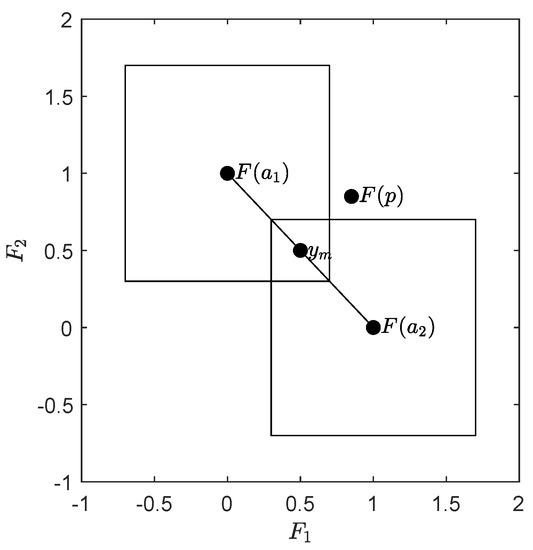 Figure 3. Linear Pareto front with slope . If for , the archive is given by such that and are the end points of the Pareto front, then the Hausdorff distance of A and the Pareto front is given by , where is the arithmetic mean of and . For , there may exist candidate solutions p that will be considered by the archive (line 5 of Algorithm 1) but discarded in the same step (lines 23 to 26 of Algorithm 1), leading to an increase of .On the one hand, one suggesting strategy would be to take as a Hausdorff approximation of the Pareto front in particular, since most Pareto fronts have at least one element where the slope of the tangent space is . On the other hand, the use of ϵ-dominance prevents that the images , , are perfectly evenly distributed along the Pareto front so that is not that accurate for some problems. In fact, this factor of two can only be observed for linear fronts, while already yields a good approximation in general (see, e.g., the subsequent results for MOPs with more than two objectives). However, we have observed that the following estimation gives even better approximations of the Hausdorff distances: given , which is sorted (e.g., according to objective ), the current Hausdorff approximation h is computed as follows:Note that the distance is set to 0 if the distance between two neighboring candidate solutions is larger or equal to , which has been done to take into account approximations of Pareto fronts that fall into several connected components.
 - (f)
- Several norms are used within the algorithm. While one is—except in line 11, see the above proof—in principle free for the choice of the norms, we suggest taking the infinity norm in line 5 in order to reduce the issue mentioned in the previous part, and the 2 norm in lines 28 and 29 in order to obtain a (slighly) better distribution of the entries along the Pareto front.
Algorithm 3 shows the modifications of ArchiveUpdateHD discussed above, which have been used for the calculations presented in this work. Hereby, denotes the vector of minimal elements for each entry .
Remark 2.
For the performance assessment of MOEAs, it is typically advisable to take instead of the Hausdorff distance the averaged Hausdorff distance . The main reason for this is that MOEAs may compute a few outliers in particular if the MOP contains weakly dominated solutions that are not optimal (also called dominance resistance solutions [72]). On the other hand, we stress that , opposed to , is not a metric in the mathematical sense, since the triangle inequality does not hold. We refer, e.g., to [13,38,73,74] for more discussion on this matter.
In the following, we discuss one possibility to obtain an approximation of the value of from a given archive A. To this end, we first investigate the value of if the elements of A are perfectly located around a linear connected Pareto front (if N is large enough, we can expect that this approximation works fine for any connected Pareto front). That is, all values are optimal. Furthermore, if A is sorted, ) and are the end points of the Pareto front, and the distance of two consecutive elements and is given by (leading to ). Since all the values are optimal, the value is hence given by the value of , which can be computed as follows:
Hereby, we have used the formulation of for continuous Pareto fronts as discussed in [73]. It remains to compute h. Since the assumption that all the images of the values are evenly spread is ideal, we cannot simply take for an arbitrarily index . Instead, it makes sense to use the average of these distances:
where is as in (12) and m denotes the number of elements of that are not equal to zero. This leads to the approximation of the averaged Hausdorff distance of the Pareto front by a given archive A:
In order to obtain a first impression on the effect of the archiver, we apply it to several test problems. More precisely, we use ArchiveUpdateHD together with the generator, which is simply choosing candidate solutions uniformly at random from the domain of the problem. As test problems, we use CONV (convex front), DENT ([75], convex-concave front), RUD1 and RUD2 (disconnected fronts), LINEAR (linear front) and RUD3 (convex front). The first five test problems are uni-modal, while RUD3 has next to the Pareto front eight local fronts. RUD3 is taken from [76], and RUD1 and RUD2 are straightforward modifications of RUD3 to obtain the given Pareto front shapes.
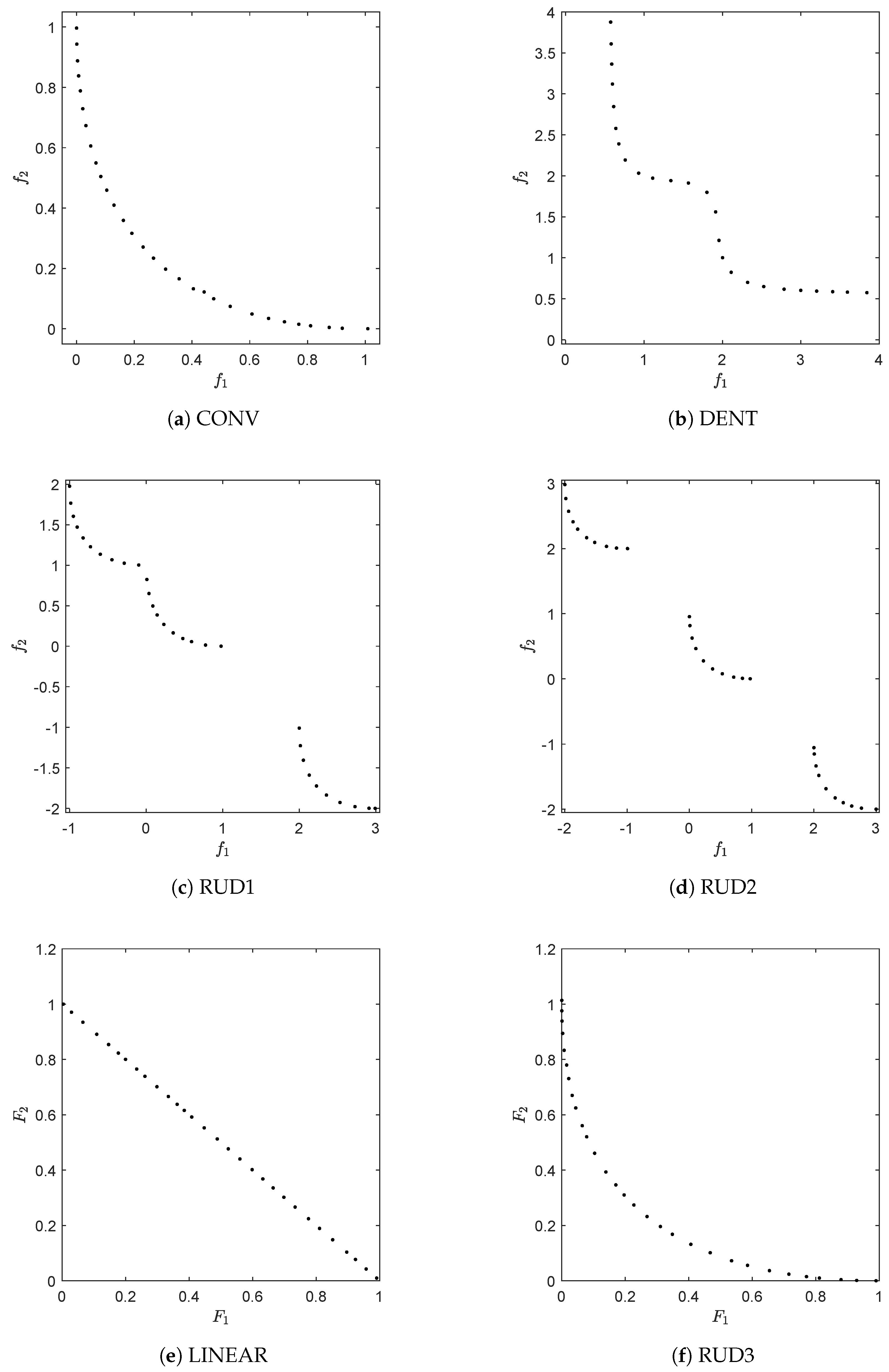
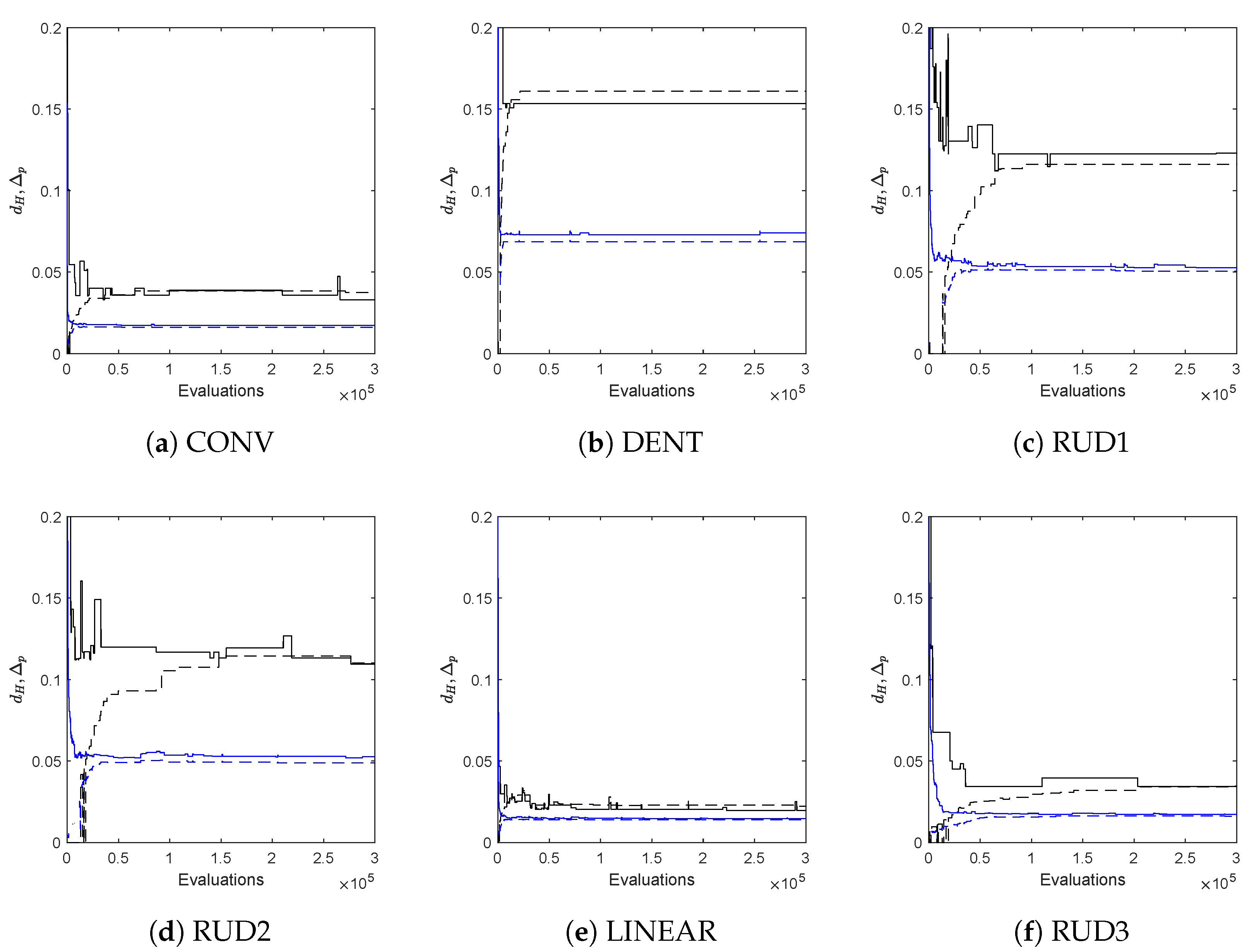
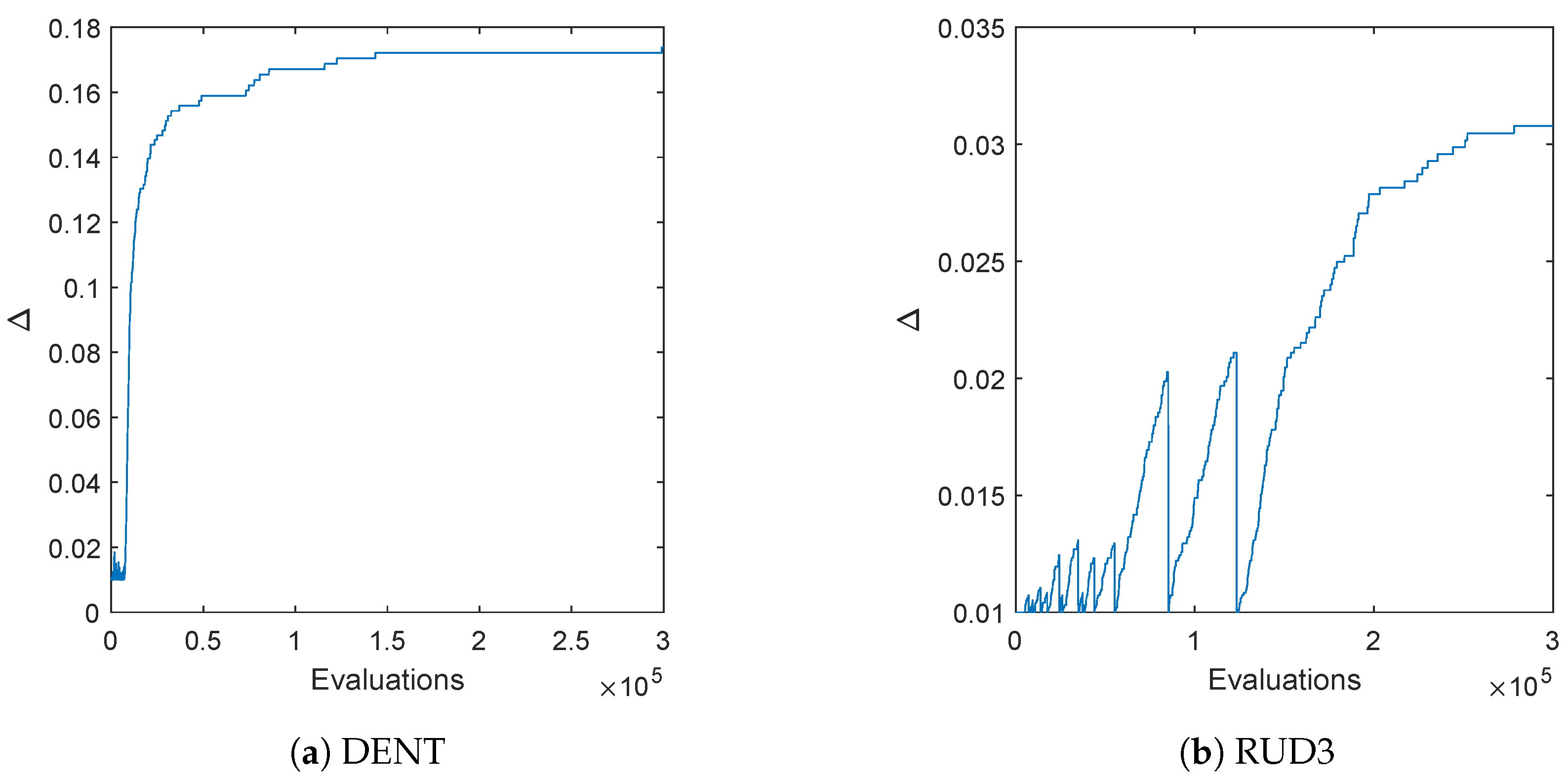
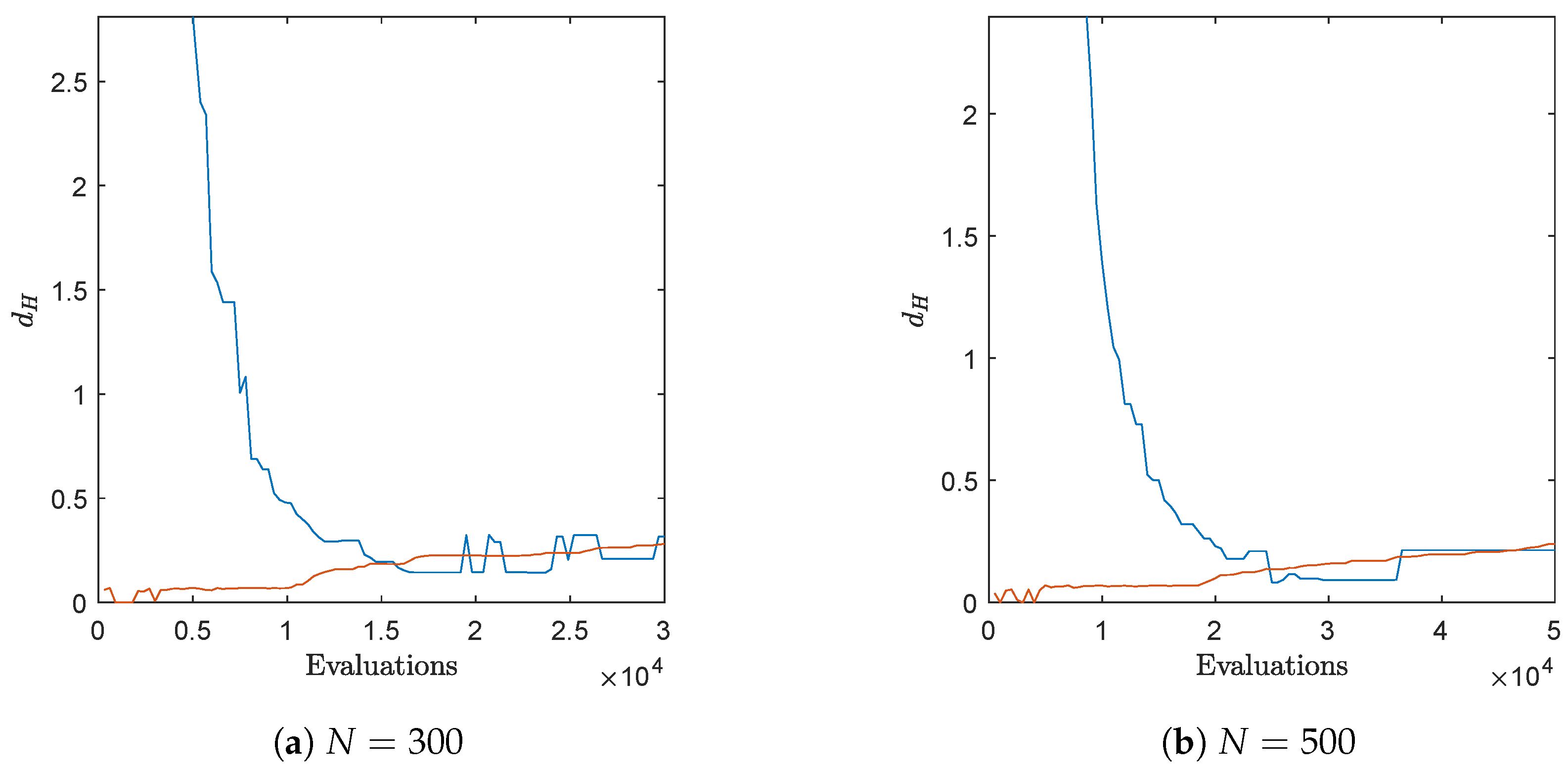
Figure 4 shows the final approximations of the fronts using for the archive size and initial values of small enough so that this threshold is reached for all problems. As it can be seen, in all cases, evenly distributed solutions along the Pareto fronts have been obtained. Figure 5 shows the actual Hausdorff and averaged Hausdorff values of the computed archives in each step for one run of the algorithm ( and , i.e., has been used for the averaged Hausdorff distance), together with their approximations h and . For all problems, the archiver is capable of quickly determining a good approximation of both and during the run of the algorithm. Table A1 and Table A2 show the approximation qualities averaged over 30 independent runs, which support the observations from Figure 5. Figure 6 shows the evolution of the value of during one run of the algorithm for DENT and RUD3. For the uni-modal problem DENT, the value of is essentially increasing monotonically (i.e., not counting the first few iteration steps), while for the multi-modal problem RUD3, more than 10 restarts occur. Nevertheless, in both cases, a final value is reached, which is in accord with Theorem 1.
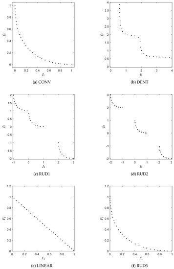
Figure 4.
Numerical results of ArchiveUpdateHD on six BOPs with different shapes of the Pareto fronts. For the sake of clarity, we omitted the fronts that already become apparent by the approximations.
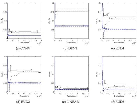
Figure 5.
Hausdorff and averaged Hausdorff approximations ( and , respectively) obtained by ArchiveUpdateHD for one single run for six bi-objective problems (see Figure 4) together with their approximations h and . is plotted black solid, h is black dashed, is blue solid, and is blue dashed.
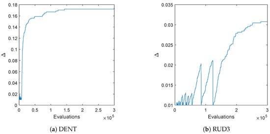
Figure 6.
Evolution of the value of for one run of the algorithm on DENT and RUD3.
Figure A1 shows the box collections
of the final archives and the final value for the test problems, where denotes the -ball around x using the maximum norm. The figure indicates that the Hausdorff distance of and the respective Pareto fronts is indeed less or equal to for all problems.
| Algorithm 3: |
| Require: Problem (MOP), where , P: current population, : current archive, : current values of , N: upper bound for archive size |
| Ensure: updated archive A, updated values for , Hausdorff approximation h |
| 1: |
| 2: |
| 3: |
| 4: for alldo |
| 5: if then |
| 6: |
| 7: end if |
| 8: for all do |
| 9: if then |
| 10: |
| 11: if then ▹ reset and |
| 12: |
| 13: |
| 14: end if |
| 15: end if |
| 16: end for |
| 17: if then ▹ apply pruning |
| 18: |
| 19: |
| 20: sort A (e.g., according to ) |
| 21: compute as in (8) |
| 22: choose |
| 23: if then |
| 24: ▹ remove 2nd entry |
| 25: else if then |
| 26: ▹ remove 2nd but last entry |
| 27: else |
| 28: |
| 29: |
| 30: if then |
| 31: |
| 32: else |
| 33: |
| 34: end if |
| 35: end if |
| 36: end if |
| 37: end for |
| 38: sort A (e.g., according to ) ▹ compute Hausdorff approximation |
| 39: compute , as in (12) |
| 40: |
| 41: return |
3.2. The General Case
Next, we consider the archiver for MOPs with more than two objectives. Algorithm 4 shows the pseudocode of ArchiveUpdateHD for such problems. The archiver is essentially identical to the one for BOPs; however, it comes with two modificatons, since one cannot expect the Pareto front to form a one-dimensional object any more and another one prevents too many unnecessary resets during the run of the algorithm.
- The distances cannot be be sorted any more as in (8). Instead, one has to consider the distancesfor a given archive A. Furthermore, more sophisticated considerations of the distances as, e.g., in lines 27 and 28 of Algorithm 3 cannot be considered any more. Instead, we have chosen to first computeand then to remove from the archiver, where l is chosen randomly from . Similar as for the bi-objective case, an exception can of course be made for the best found solutions for each objective value.
- The approximation of the Hausdorff distance cannot be done as in (12) any more. Instead, we choose the value of as an approximation for , which is motivated by Theorem 1.
- The reset is completed if there exists an entry a of the current archive A and a candidate solution p that dominates a andThat is, the improvement is larger than for all objectives. It has been observed that if one only asks for an improvement in one objective (as done for the bi-objective case), too many resets are performed in particular for MOPs that contain a “flat” region of the Pareto front.
Note that none of these changes affects the statements made in Theorem 1. Hence, the statements of Theorem 1 also hold if Algorithm 4 is used for MOPs with objectives. We stress that this algorithm can of course also be used for the treatment of BOPs; however, in that case, Algorithm 3 seems to be better suited, since both distance considerations and Hausdorff approximation are more sophisticated.
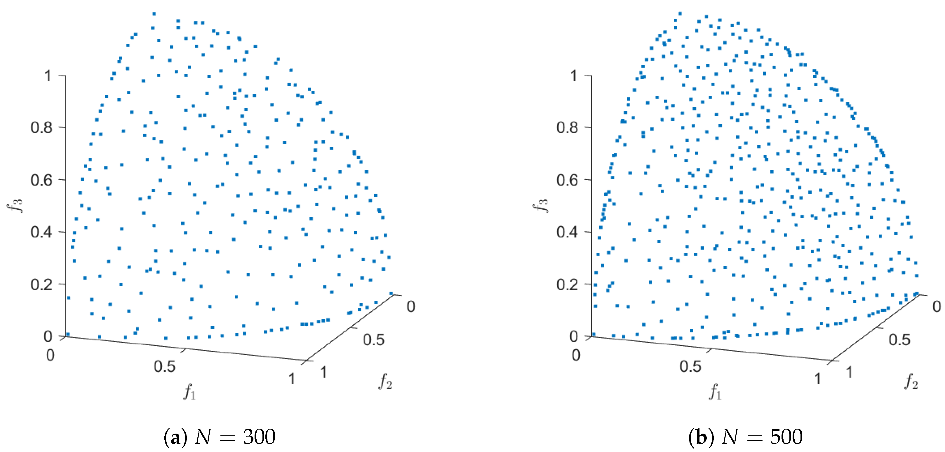
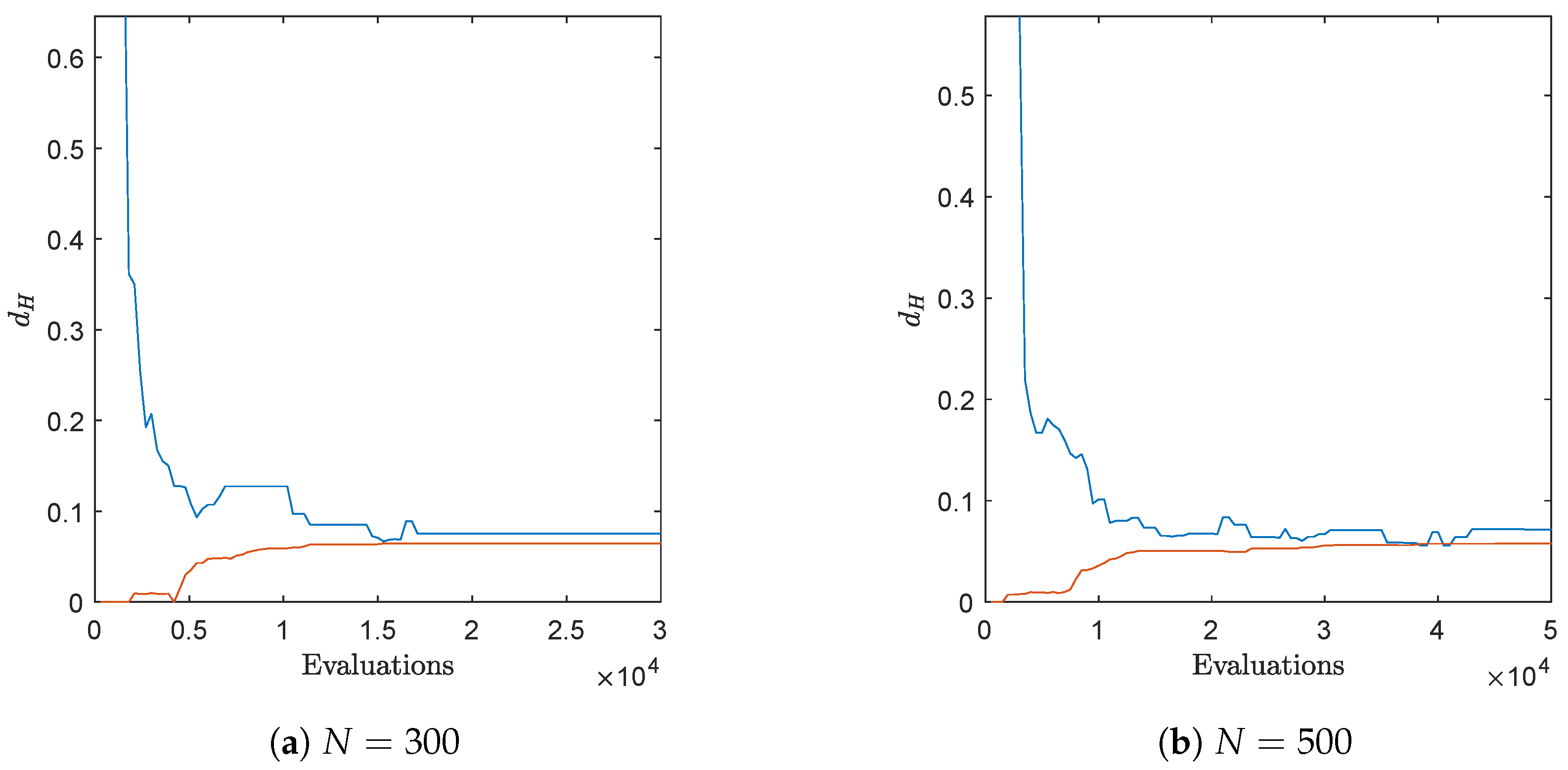
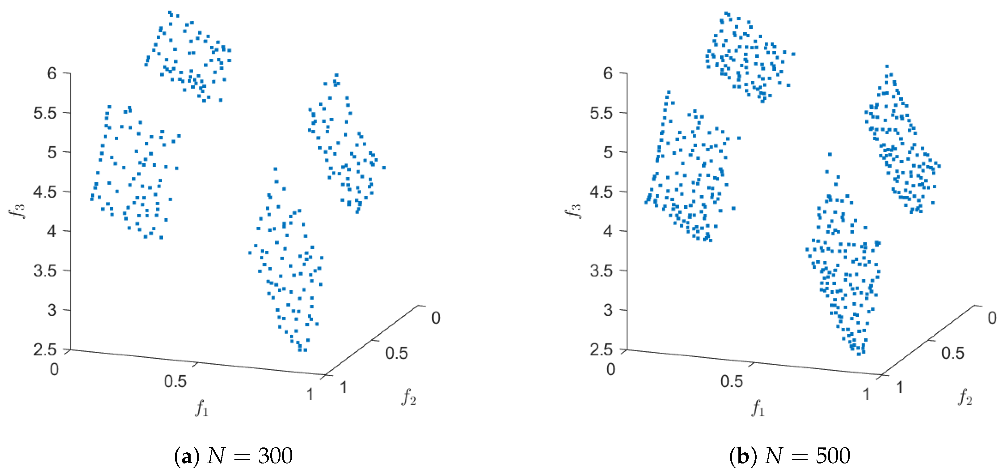
Figure 7 shows an application of Algorithm 4 on the test function DTLZ2 with three objectives (concave and connected Pareto front) for and . The evolution of the approximated value of the Hausdorff distance together with the real value can be found in Figure 8. Hereby, we have used ArchiveUpdateHD as the external archiver of NSGA-II. The same result could have been obtained using randomly chosen test points within the domain Q, however, for a much higher amount of test points. Figure 9 and Figure 10 show the respective results for DTLZ7, whose Pareto front is disconnected and convex-concave. In all cases, the archiver is capable of finding evenly spread solutions along the Pareto front, and the value of is already after some iterations quite close to the actual Hausdorff distance. In order to suitably handle weakly optimal solutions, we have used the approach we describe in the following remark.
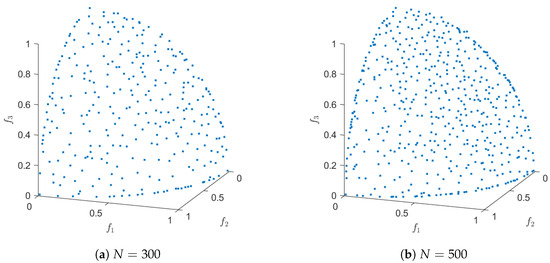
Figure 7.
Results of ArchiveUpdateHD on DTLZ2 for different values of N.
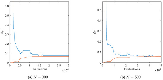
Figure 8.
Real (blue) and approximated (red) Hausdorff distances during the run of one algorithm for DTLZ2.
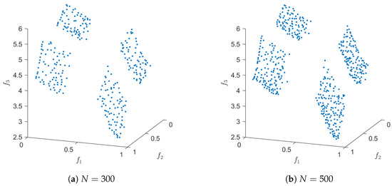
Figure 9.
Results of ArchiveUpdateHD on DTLZ7 for different values of N.
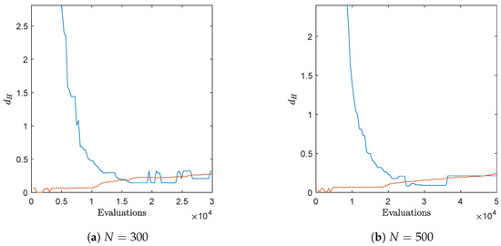
Figure 10.
Real (blue) and approximated (red) Hausdorff distances during the run of one algorithm for DTLZ7.
Remark 3.
It is known that distance-based archiving/selection for MOPs that contains weakly optimal solutions that are not optimal (dominance-resistant solutions) may lead to unsatisfactory results, since candidates may be included in the archive that are far away from the Pareto front. In [77], it has been suggested to consider the modified objectives
where is “small”, instead of the orginal objectives , . We have adopted this approach for the treatment of the ZDT and DTLZ functions in this work, using .
| Algorithm 4 |
| Require: Problem (MOP), P: current population, : current archive, : current value of , N: upper bound for archive size |
| Ensure: updated archive A, updated value of |
| 1: |
| 2: |
| 3: |
| 4: for all do |
| 5: if then |
| 6: |
| 7: end if |
| 8: for all do |
| 9: if then |
| 10: |
| 11: if , then ▹ reset and |
| 12: |
| 13: |
| 14: end if |
| 15: end if |
| 16: end for |
| 17: if then ▹ apply pruning |
| 18: |
| 19: |
| 20: compute as in (17) |
| 21: choose |
| 22: choose l randomly from |
| 23: |
| 24: end if |
| 25: end for |
| 26: return |
Remark 4.
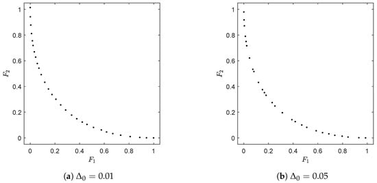
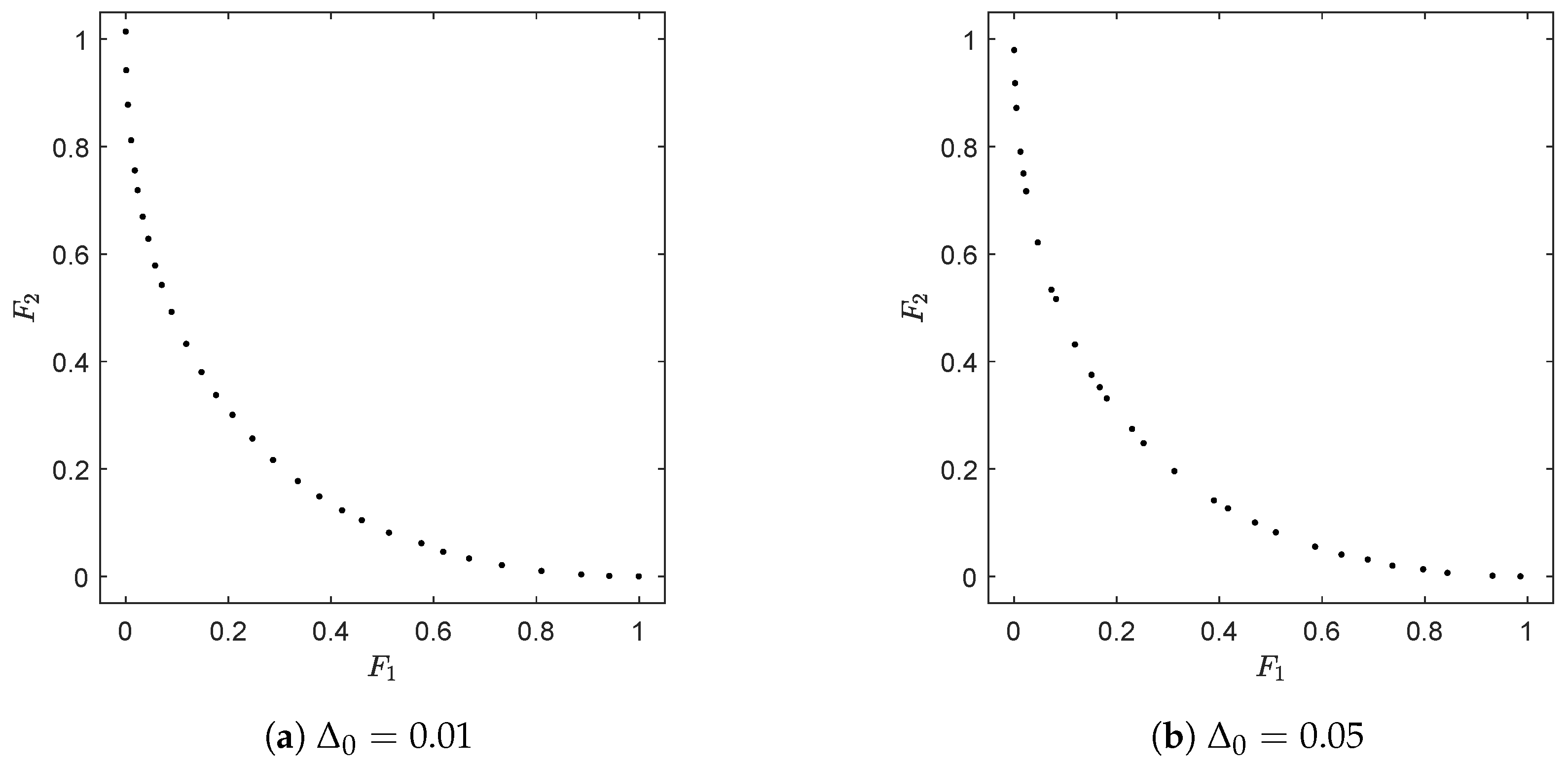
We finally stress that the archiver A only reaches the magnitude N if Δ (and hence ϵ) is chosen “small enough”, which does not represent a drawback in our opinion. In real-world applications, the values of Δ have a physical meaning. As a hypothetical example, consider that one objective in the design of the car is its maximal speed (e.g., ), and the decision maker considers two cars to have different maximal speeds if differs by at least 10 km/h. In this case is a suitable choice for ArchiveUpdateHD. Hence, depending on these values and the size of the Pareto front, it may happen that less than N elements are needed to suitably represent the solution set. In turn, if is (significantly) larger than the target values, this gives a hint to the decision maker that N has to be increased and that the computation has to be repeated in order to obtain a “complete” approximation. Figure 11 shows two results of ArchiveUpdateHD on CONV for two different starting values of Δ.

Figure 11.
Results of ArchiveUpdateHD on CONV for two different initial values of using . For , the final archive contains 30 elements, while there are only 28 elements for . The solutions on the left are more evenly spread along the Pareto front due to distance considerations in the pruning technique. For the solution on the right, no pruning technique has been applied during the run of the algorithm.
4. Numerical Results
In this section, we show some more numerical results to further demonstrate the advantage of the proposed archiver. As base MOEAs, we have chosen to take the state-of-the-art algorithms NSGA-II (dominance based), MOEA/D (decomposition based), and SMS-EMOEA (indicator based). We have used the implementations of the algorithms as well as the reference fronts provided by PlatEMO [78]. For sake of a fair comparison, we will in the following equip these MOEAs with ArchiveUpdateHD as an external archiver, where the upper bound N is chosen equal to the population sizes. For each run of an algorithm, we have fed the archiver with exactly the same candidate solution as for the respective base MOEA.
Motivated by Theorem 1 and by the discussion made in Remark 2, we will primarily use () for the performance assessment of the MOEA results. However, we will also use the Hpyervolume indicator [79], leading to some surprising results.
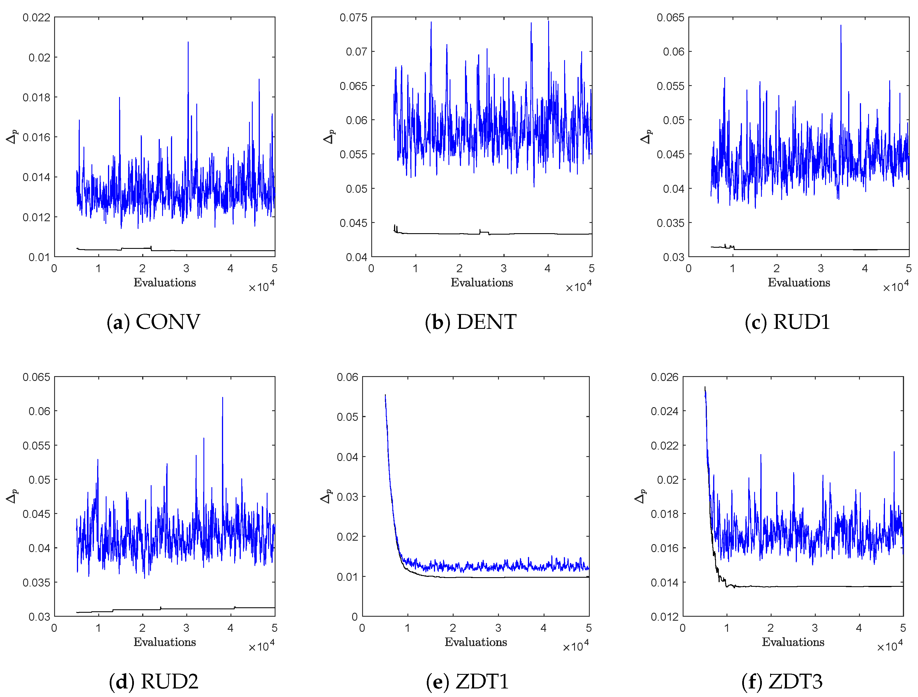
We first make a comparison with NSGA-II to investigate possible cyclic behavior during the run of an algorithm. It is known that distance-based selection/archiving strategies may lead to such cyclic behavior, which means that from a certain stage of the search, no more improvements can be expected (and in particular no convergence). The selection strategy of NSGA-II is mainly distance based (since from a certain point on, all individuals of the population are mutually non-dominated). For this, we have set both population size and N to 50 and have run NSGA-II for 1000 generations, using and for SBX, and and for polynomial mutation. For ArchiveUpdateHD, we have chosen the first small enough so that archive size was reached for all problems. In Figure 12, typical evolutions of the values of the approximation qualities are shown over time for six selected BOPs (similar plots are obtained for all problems considered in this study). Hereby, “NSGA-II” stands for the population of the MOEA, and “NSGA-II-A” stands for the respective archive that was fed with the same candidate solutions as NSGA-II. While NSGA-II reveals clear cyclic behavior in all cases, this is not the case for NSGA-II-A. The latter is due to the acceptance strategy of ArchiveUpdateHD that is based on -dominance. As discussed above, the value of (and hence also of ) will become large enough during the run of the algorithm so that only dominance replacements will occur, which, however, cannot lead to cyclic behavior.

Figure 12.
Approximation qualities of the Pareto fronts (measured by ) during one run of the algorithm for NSGA-II (blue) and the archives NSGA-II-A (black) for six selected BOPs.
Apart from the “quasi-monotonic” behavior, one can also observe that the values of NSGA-II-A are for all test problems significantly lower than the ones of NSGA-II.
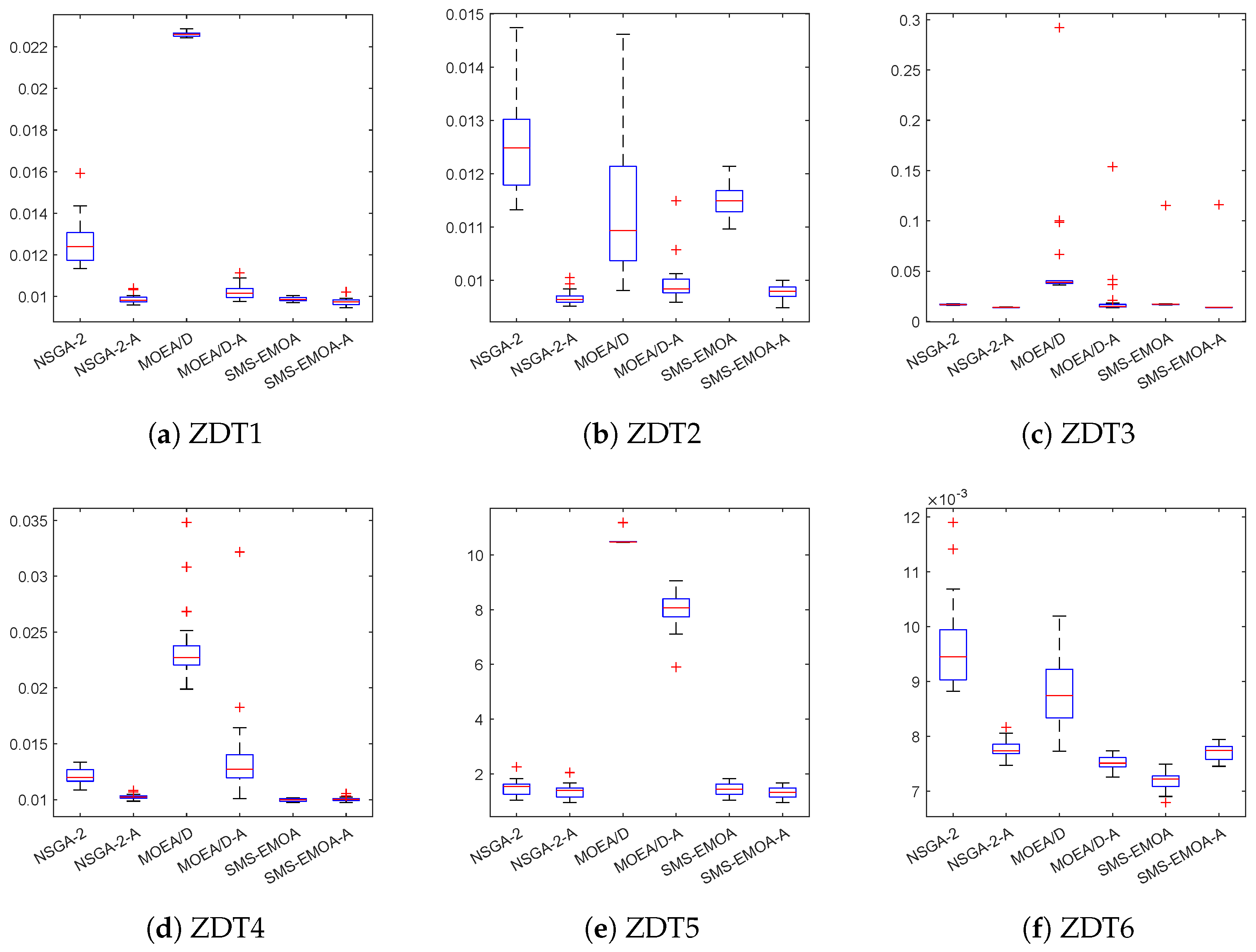
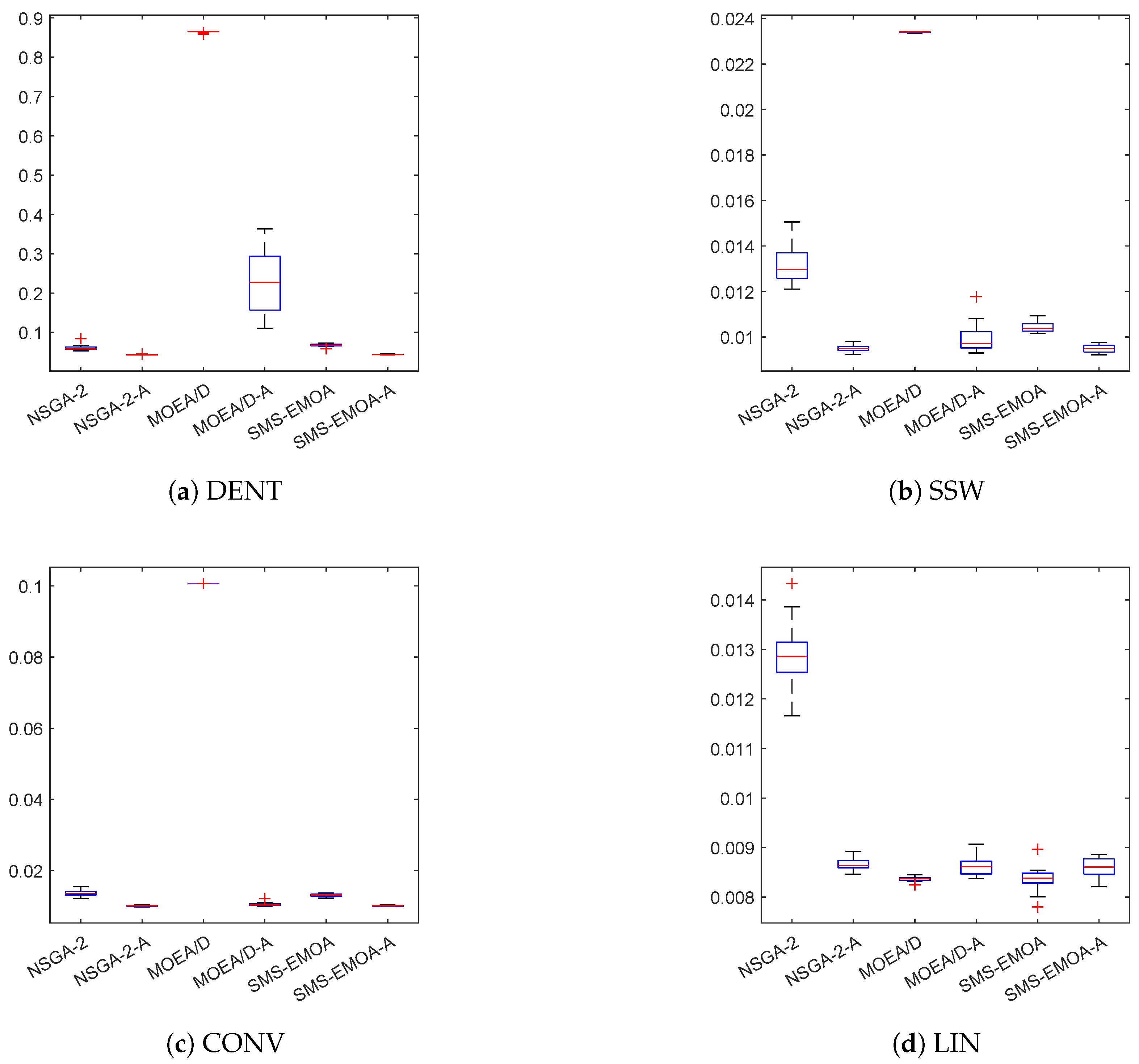
Next, we investigate the performance of ArchiveUpdateHD as an external archive for the three MOEAs using an extended set of test functions. We first consider bi-objective problems. For this, we have chosen the ZDT problems [80], where we have used the modified objectives as expressed in (19) using to handle weak Pareto optimal solutions that are not optimal. Next to these six test problems, we have taken another four BOPs, which were selected due to the shapes of their fronts: LIN ([81], linear front), CONV (convex front), as well as DENT and SSW [82], which have both convex–concave Pareto fronts. The boxplots of the results are shown in Figure 13 and Figure 14, based on 30 independent runs, for each using 1000 generations and a population size of 50. The Wilcoxon rank-sum is shown in Table 1. In the following, we will compare the results of the base algorithms against the respective solutions that use ArchiveUpdateHD.
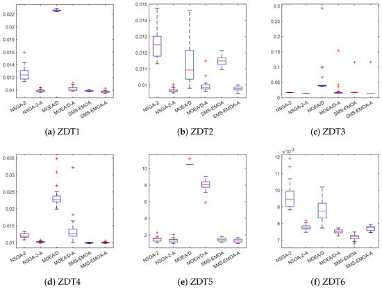
Figure 13.
Boxplots for the obtained results for the ZDT test functions.
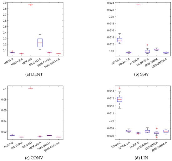
Figure 14.
Boxplots for the obtained results for DENT, SSW, CONV and LIN.

Table 1.
Comparison (wins/ties/losses) of the results of the base MOEAs against their archive equipped variants on the bi-objective test problems. The Wilcoxon rank-sum test has been used for statistical significance, where p-value .
The performance of the external archives is better in 10 out of 10 cases for NSGA-II, in 9 out of 10 cases for MOEA/D, and in 8 out of 10 cases for SMS-EMOA. ArchiveUpdateHD loses against the MOEA/D and SMS-EMOA on test problem LIN, which has a linear and thus most possible regular Pareto front. Both MOEA/D and SMS-EMOA are able to compute perfect solutions for this problem. Such perfect approximations cannot be expected from ArchiveUpdateHD due to its acceptance strategy. While this strategy is responsible for suppressing any cyclic behavior, it also prevents that all the solutions even of the limit archive are perfectly evenly spread along the Pareto front. For more complex Pareto fronts, the situation, however, changes. Figure A2 and Figure A3 show the average results obtained by the different methods on problems DENT and ZDT, respectively. For DENT, the use of ArchiveUpdateHD leads in all three cases to significantly better Pareto front approximations. This is similar to ZDT3, while the improvements are less, since all three base MOEAs can already detect very good approximations.
In a next step, we investigate the effect of ArchiveUpdateHD on several test problems with objectives. For this, we have chosen the seven DLTZ test problems, the test functions IDTLZ1 and ITDLZ2 [21] with “inverted” fronts, and MaF1 to 5 [83]. Table 2 shows the Wilcoxon rank-sum for these 14 test problems using the indicators , HV, as well as the classical Hausdorff distance . Figure A4 shows the boxplots for all algorithms and test problems for , Figure A5 and Figure A6 show the results of the algorithms on IDTLZ1 and MaF2, respectively, and Figure A7 shows the selected behaviors of the Hausdorff approximations. For the latter, we have taken the median runs with respect to . As it can be seen from Table 2, the use of ArchiveUpdateHD as the external archiver is highly beneficial in almost all cases. More precisely, starting with , NSGA-II-A is better than NSGA-II in 12 out of 14 cases, and it only becomes (slightly) beaten on DTLZ5 and 6, which is likely owed to the degeneration the Pareto fronts of these two test problems (which has to be investigated in more detail in the future). MOEAD-A is superior to MOEAD in 10 out of 14 cases with one tie (DTLZ4) and 3 losses (DLTZ1-3), which is due to the regular structure of these Pareto fronts where MOEA/D can hardly be beaten. Finally, SMS-EMOA-A yields better results in all of the 14 cases. The situation is quite similar when considering the other two performance indicators. While this was expected for , the results are surprising for HV: note that SMS-EMOA-A also outperforms SMS-EMOA on all of the 14 test functions when considering the hypervolume indicator.

Table 2.
Comparison (wins (1) / ties (0) / losses (−1)) of the results of the base MOEAs against their archive equipped variants on the 14 three-objective test problems. The Wilcoxon rank-sum test has been used for statistical significance, where p-value .
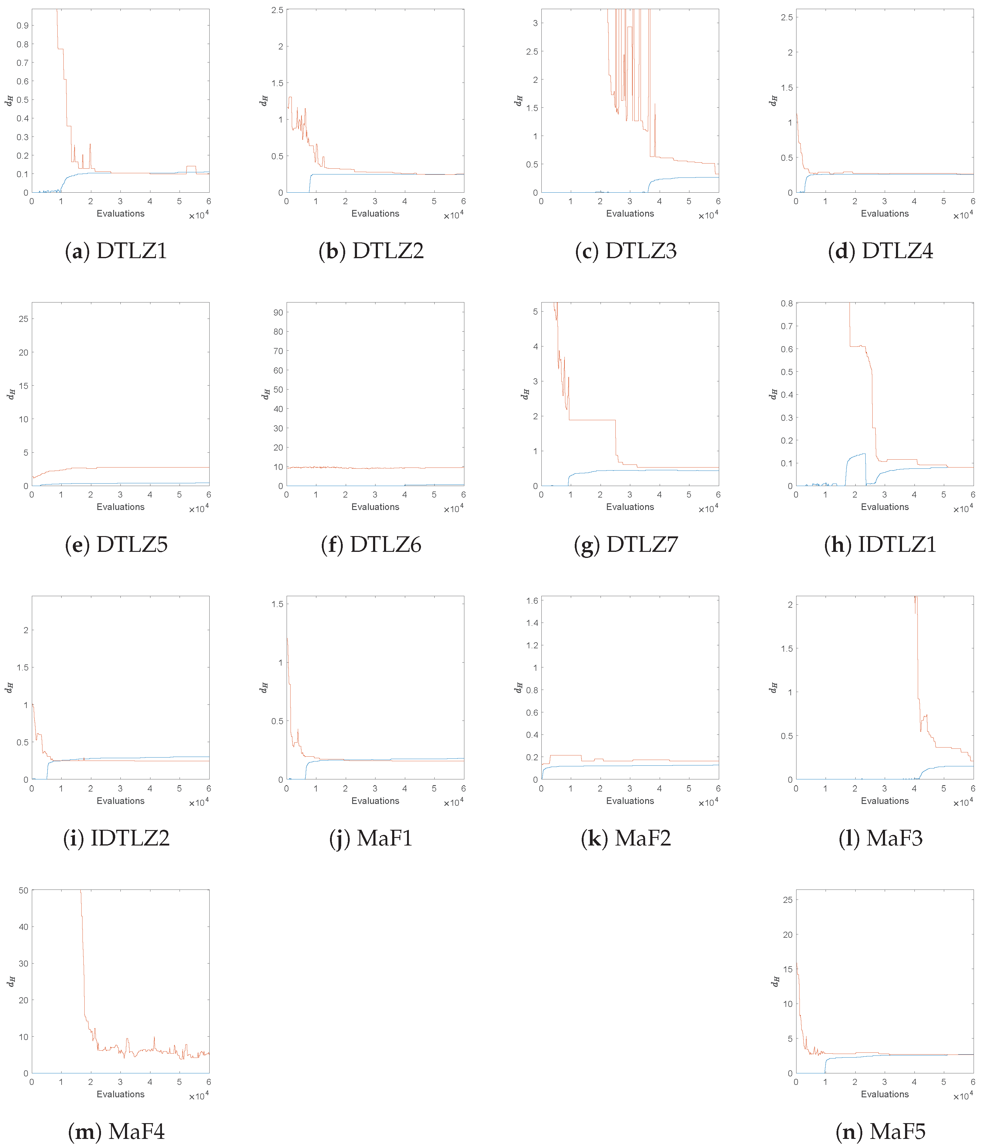
Finally, Figure A8 and Figure A9 show evolutions of the obtained Hausdorff distances of NSGA-II-A for the same test problems but now using and objectives. The results already give evidence that the values of obtained by ArchiveUpdateHD yield satisfying approximations of the actual values of also for problems with more objectives. The only exceptions are DTLZ5 and DTLZ6 (both for four and five objectives) as well as MaF4 for . By Theorem 1, we know that the runs of the algorithms have simply not been long enough, while it is in turn unclear how long these runs should have been. While these results are satisfying, more investigation has to be done in particular for the treatment of many objective problems, which we leave for future study.
5. Conclusions and Future Work
In this paper, we have presented and analyzed the archiving strategy ArchiveUpdateHD for use within set-based stochastic search algorithms such as multi-objective evolutionary algorithms (MOEAs) for the treatment of multi-objective optimization problems (MOPs). ArchiveUpdateHD is a bounded archiver that is based on distance dominance, -dominance and the distances among the candidate solutions and that aims for evenly spread solutions along the Pareto front of a given MOP. We have shown that the images of the sequence of archives generated by this archiver form under certain (mild) conditions of the process to generate candidate solutions with a probability of one of a -approximation of the Pareto front in the Hausdorff sense, and all entries of converge to Pareto optimal solutions with a probability of one and for . Furthermore, the value is computed by ArchiveUpdateHD during the run of the algorithm (without any prior knowledge of the Pareto front). Since this value represents the maximal error in the representation, it is of important value for the decision maker (DM). In particular, if the magnitude of the archives reaches the pre-defined value N, the value of gives a feedback if the approximation is “complete enough” or not. Empirical studies on several benchmark test problems have shown the benefit of the novel strategy, among others, that the obtained value gives a good approximation of the actual Hausdorff approximation. For bi-objective problems, we have presented an alternative way to compute this value, which can even be considered to be tight from the practical point of view. Finally, we have used ArchiveUpdateHD as the external archiver for three state-of-the-art MOEAs (NSGA-II, MOEA/D, and SMS-EMOA), indicating that it is capable of significantly improving the overall performance of these algorithms.
One important next step which we will leave for future work is to use the mechanisms behind ArchiveUpdateHD as the selection strategy within an MOEA. If an external archiver is used, two archives (instead of only one) have to be maintained, leading to an additional overhead, which could be avoided. It is hence intended to utilize ArchiveUpdateHD to design a new class of MOEAs that aims for (averaged) Hausdorff approximations of the Pareto fronts (as, e.g., done in [84,85,86]).
Author Contributions
C.I.H.C. and O.S. have contributed equally to this work. All authors have read and agreed to the published version of the manuscript.
Funding
This research received no external funding.
Data Availability Statement
The codes will be made publicly available after acceptance.
Conflicts of Interest
The authors declare no conflict of interest.
Appendix A

Table A1.
Hausdorff distances and approximations h computed by ArchiveUpdateHD for the six bi-objective problems.
Table A1.
Hausdorff distances and approximations h computed by ArchiveUpdateHD for the six bi-objective problems.
| Problem | Mean | std | Mean h | std h |
|---|---|---|---|---|
| CONV | 0.0345 | 0.0014861 | 0.036105 | 0.0016771 |
| DENT | 0.15428 | 0.012059 | 0.15872 | 0.0091187 |
| RUD1 | 0.11337 | 0.0075653 | 0.10027 | 0.024311 |
| RUD2 | 0.11295 | 0.0083812 | 0.085445 | 0.038149 |
| LINEAR | 0.02094 | 0.0019671 | 0.01977 | 0.0068899 |
| RUD3 | 0.035354 | 0.0023404 | 0.025694 | 0.011484 |

Table A2.
Averaged Hausdorff distances and approximations computed by ArchiveUpdateHD for the six bi-objective problems.
Table A2.
Averaged Hausdorff distances and approximations computed by ArchiveUpdateHD for the six bi-objective problems.
| Problem | Mean | std | Mean | std |
|---|---|---|---|---|
| CONV | 0.016626 | 0.00021014 | 0.01602 | 4.9072 |
| DENT | 0.070802 | 0.00075385 | 0.069309 | 0.00036096 |
| RUD1 | 0.052171 | 0.00072633 | 0.050631 | 0.0022879 |
| RUD2 | 0.050967 | 0.00068389 | 0.049108 | 0.00034928 |
| LINEAR | 0.014494 | 0.00033184 | 0.013892 | 0.00018454 |
| RUD2 | 0.016653 | 0.00028272 | 0.01595 | 0.00034355 |
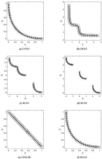
Figure A1.
The box coverings for the final archives incidate that the Hausdorff distance between and the Pareto fronts is less than the final value computed by ArchiveUpdateHD for all test problems.
Figure A1.
The box coverings for the final archives incidate that the Hausdorff distance between and the Pareto fronts is less than the final value computed by ArchiveUpdateHD for all test problems.
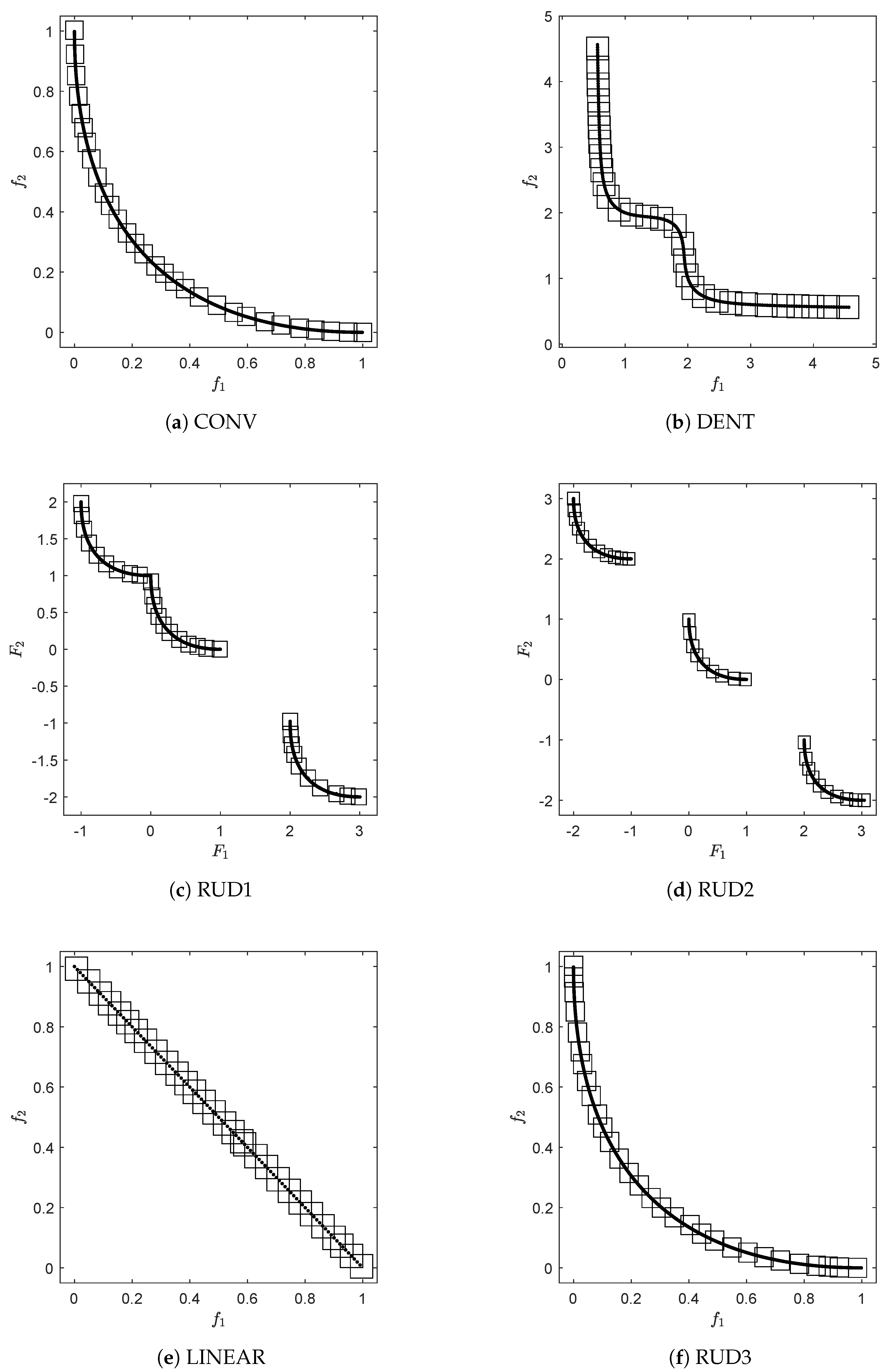
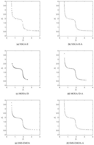
Figure A2.
Numerical results of the different algorithms and archiving/selection strategies on DENT.
Figure A2.
Numerical results of the different algorithms and archiving/selection strategies on DENT.


Figure A3.
Numerical results of the different algorithms and archiving/selection strategies on ZDT3.
Figure A3.
Numerical results of the different algorithms and archiving/selection strategies on ZDT3.
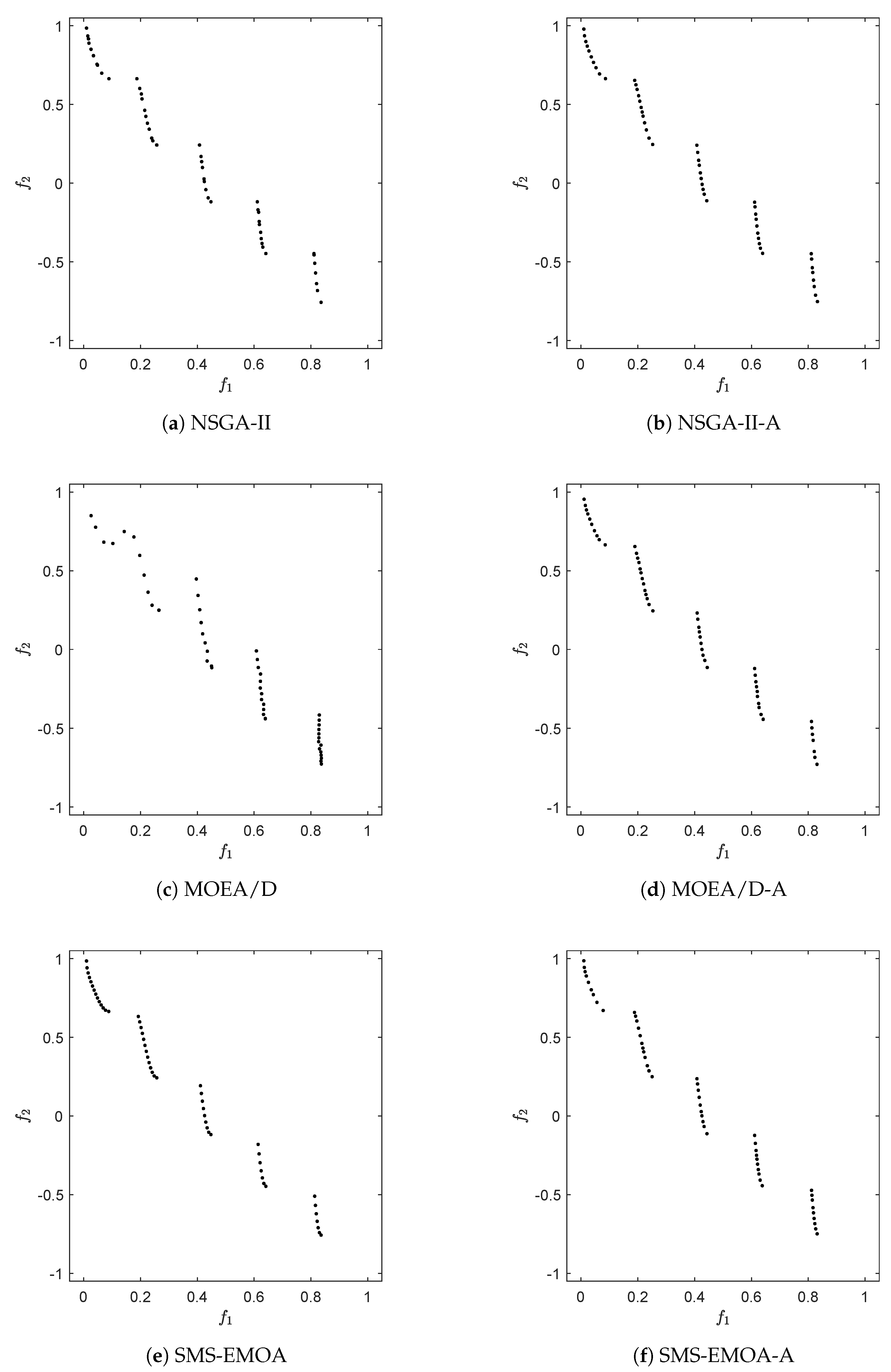
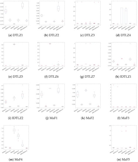
Figure A4.
Boxplots for the considered three-objective test functions.
Figure A4.
Boxplots for the considered three-objective test functions.
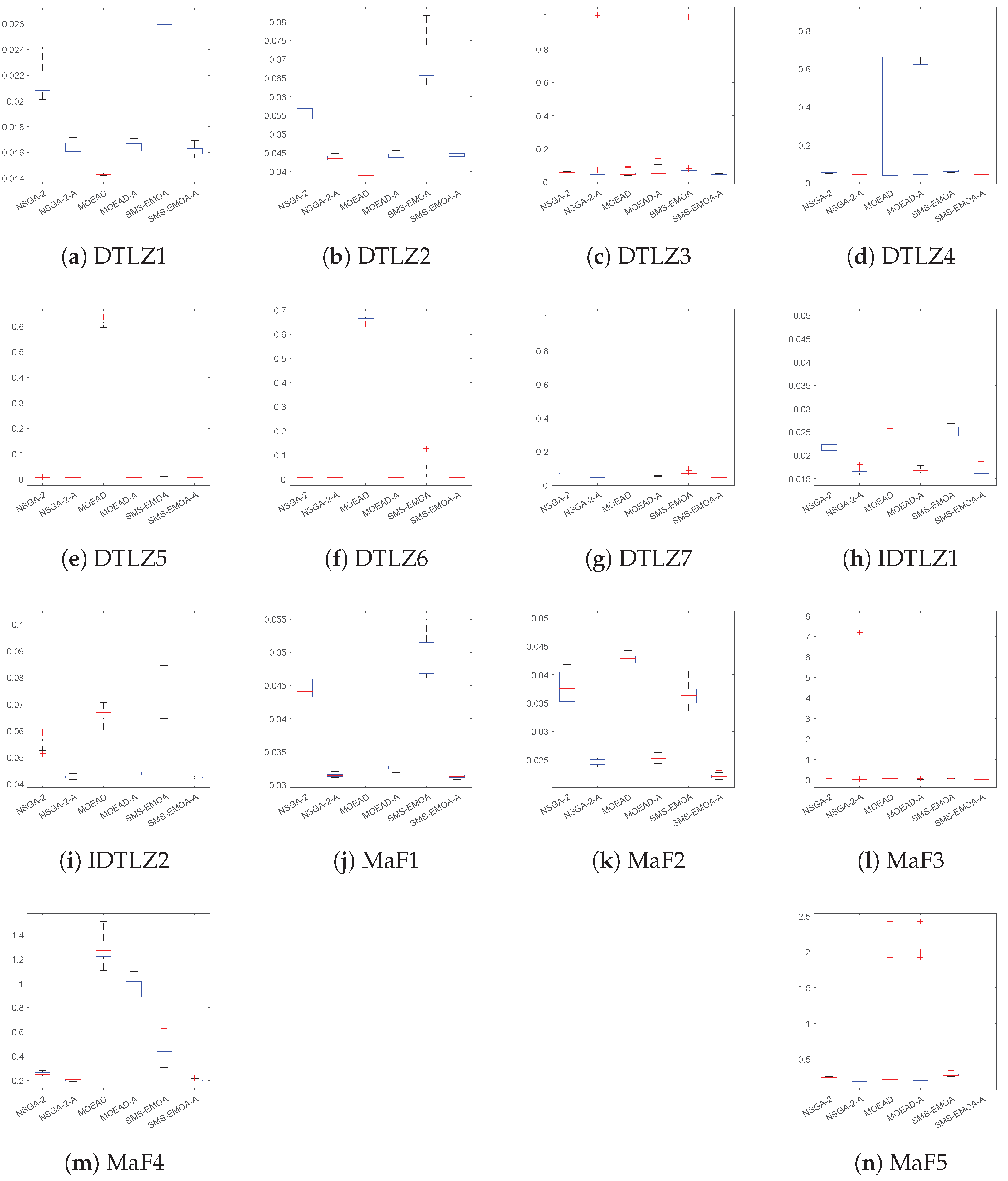
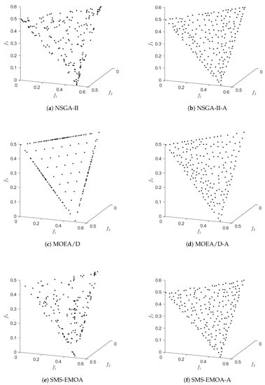
Figure A5.
Numerical results of the different algorithms and archiving/selection strategies on IDTLZ1 for .
Figure A5.
Numerical results of the different algorithms and archiving/selection strategies on IDTLZ1 for .

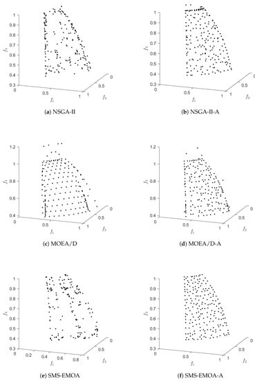
Figure A6.
Numerical results of the different algorithms and archiving/selection strategies on MaF2 for .
Figure A6.
Numerical results of the different algorithms and archiving/selection strategies on MaF2 for .
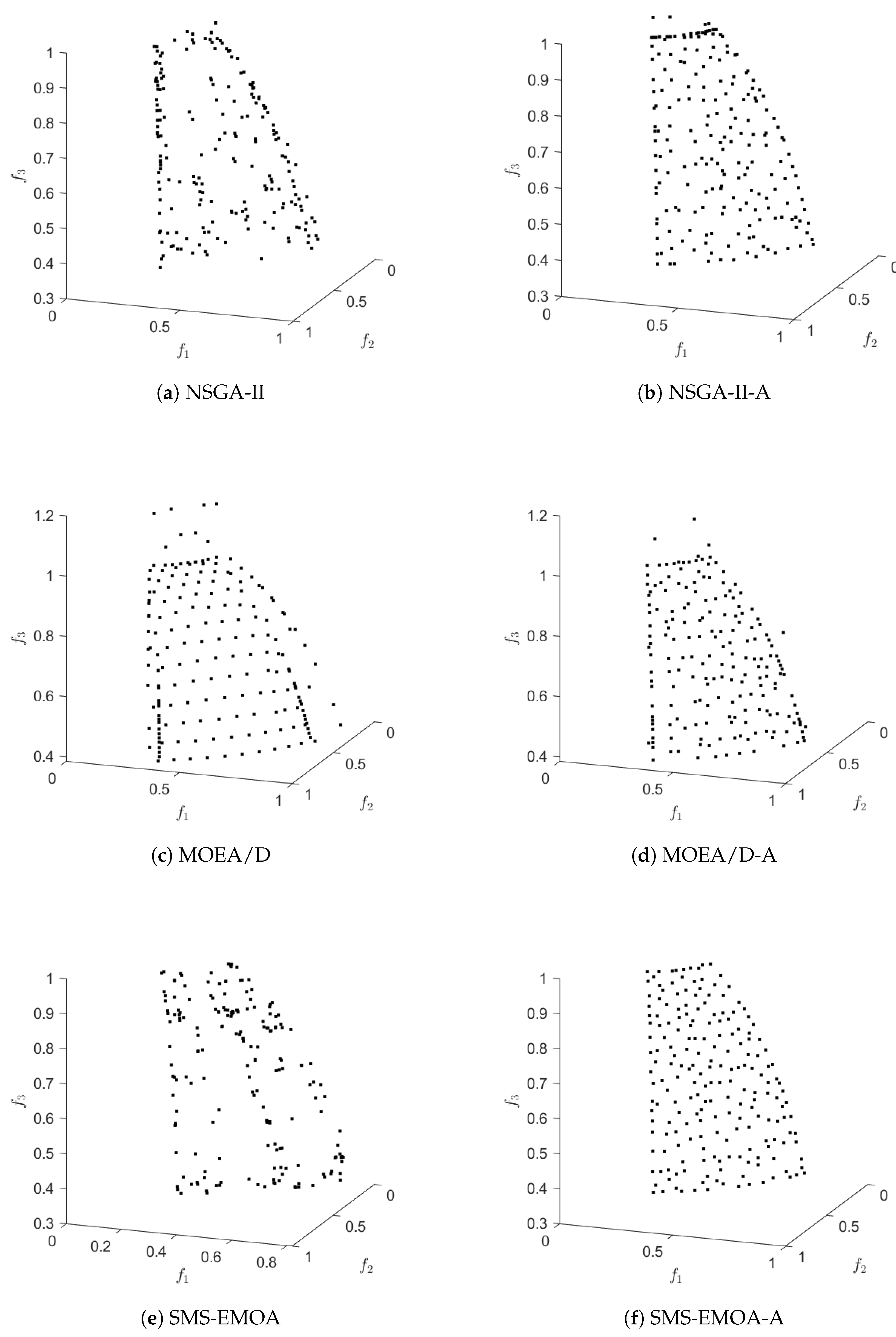
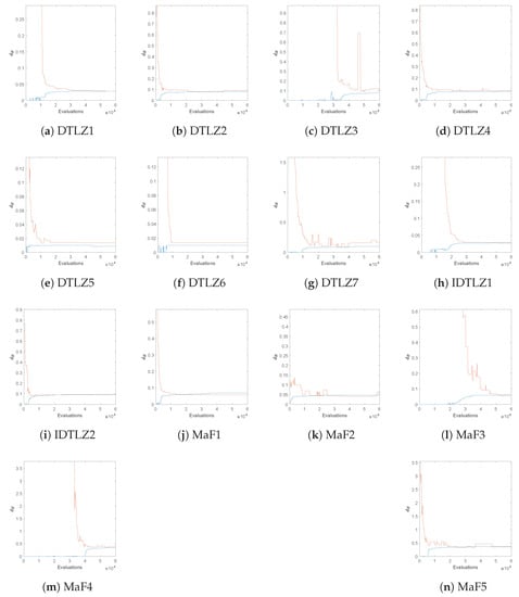
Figure A7.
Evolution of the Hausdorff distances of NSGA-II-A and the computed approximations for several test functions, using objectives.
Figure A7.
Evolution of the Hausdorff distances of NSGA-II-A and the computed approximations for several test functions, using objectives.
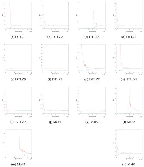
Figure A8.
Evolution of the Hausdorff distances of NSGA-II-A and the computed approximations for several test functions, using objectives.
Figure A8.
Evolution of the Hausdorff distances of NSGA-II-A and the computed approximations for several test functions, using objectives.
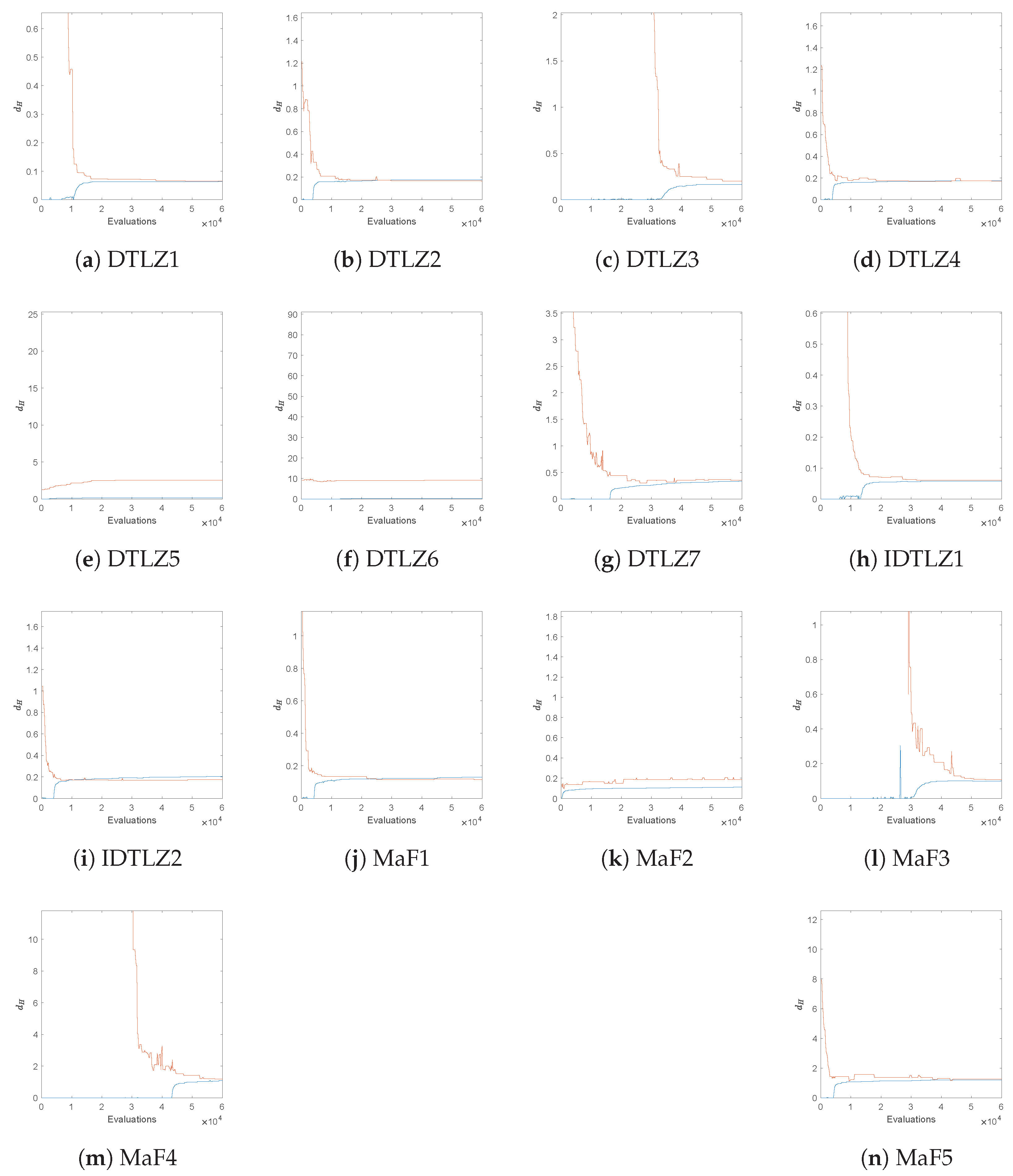
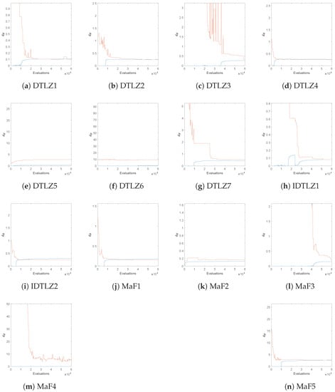
Figure A9.
Evolution of the Hausdorff distances of NSGA-II-A and the computed approximations for several test functions, using objectives.
Figure A9.
Evolution of the Hausdorff distances of NSGA-II-A and the computed approximations for several test functions, using objectives.
References
- Laumanns, M.; Thiele, L.; Deb, K.; Zitzler, E. Combining convergence and diversity in evolutionary multiobjective optimization. Evol. Comput. 2002, 10, 263–282. [Google Scholar] [CrossRef] [PubMed]
- Deb, K. Multi-Objective Optimization Using Evolutionary Algorithms; John Wiley & Sons: Chichester, UK, 2001; ISBN 0-471-87339-X. [Google Scholar]
- Stewart, T.; Bandte, O.; Braun, H.; Chakraborti, N.; Ehrgott, M.; Göbelt, M.; Jin, Y.; Nakayama, H. Real-World Applications of Multiobjective Optimization. In Proceedings of the Multiobjective Optimization; Lecture Notes in Computer Science; Slowinski, R., Ed.; Springer: Berlin/Heidelberg, Germany, 2008; Volume 5252, pp. 285–327. [Google Scholar]
- Sun, J.Q.; Xiong, F.R.; Schütze, O.; Hernández, C. Cell Mapping Methods—Algorithmic Approaches and Applications; Springer: Berlin/Heidelberg, Germany, 2019. [Google Scholar]
- Aguilera-Rueda, V.J.; Cruz-Ramírez, N.; Mezura-Montes, E. Data-Driven Bayesian Network Learning: A Bi-Objective Approach to Address the Bias-Variance Decomposition. Math. Comput. Appl. 2020, 25, 37. [Google Scholar] [CrossRef]
- Estrada-Padilla, A.; Lopez-Garcia, D.; Gómez-Santillán, C.; Fraire-Huacuja, H.J.; Cruz-Reyes, L.; Rangel-Valdez, N.; Morales-Rodríguez, M.L. Modeling and Optimizing the Multi-Objective Portfolio Optimization Problem with Trapezoidal Fuzzy Parameters. Math. Comput. Appl. 2021, 26, 36. [Google Scholar] [CrossRef]
- Frausto-Solis, J.; Hernández-Ramírez, L.; Castilla-Valdez, G.; González-Barbosa, J.J.; Sánchez-Hernández, J.P. Chaotic Multi-Objective Simulated Annealing and Threshold Accepting for Job Shop Scheduling Problem. Math. Comput. Appl. 2021, 26, 8. [Google Scholar] [CrossRef]
- Castellanos-Alvarez, A.; Cruz-Reyes, L.; Fernandez, E.; Rangel-Valdez, N.; Gómez-Santillán, C.; Fraire, H.; Brambila-Hernández, J.A. A Method for Integration of Preferences to a Multi-Objective Evolutionary Algorithm Using Ordinal Multi-Criteria Classification. Math. Comput. Appl. 2021, 26, 27. [Google Scholar] [CrossRef]
- Hillermeier, C. Nonlinear Multiobjective Optimization: A Generalized Homotopy Approach; Springer Science & Business Media: Berlin/Heidelberg, Germany, 2001; Volume 135. [Google Scholar]
- Coello Coello, C.A.; Lamont, G.B.; Van Veldhuizen, D.A. Evolutionary Algorithms for Solving Multi-Objective Problems, 2nd ed.; Springer: New York, NY, USA, 2007. [Google Scholar]
- Laumanns, M.; Zenklusen, R. Stochastic convergence of random search methods to fixed size Pareto front approximations. Eur. J. Oper. Res. 2011, 213, 414–421. [Google Scholar] [CrossRef]
- Hernández, C.; Schütze, O. A Bounded Archive Based for Bi-objective Problems based on Distance and epsilon-dominance to avoid Cyclic Behavior. In Proceedings of the Genetic and Evolutionary Computation Conference (GECCO-2022), Boston, MA, USA, 9–13 July 2022. [Google Scholar]
- Schütze, O.; Esquivel, X.; Lara, A.; Coello, C.A.C. Using the averaged Hausdorff distance as a performance measure in evolutionary multi-objective optimization. IEEE Trans. Evol. Comput. 2012, 16, 504–522. [Google Scholar] [CrossRef]
- Schütze, O.; Laumanns, M.; Tantar, E.; Coello, C.A.C.; Talbi, E.G. Computing gap free Pareto front approximations with stochastic search algorithms. Evol. Comput. 2010, 18, 65–96. [Google Scholar] [CrossRef]
- Deb, K.; Pratap, A.; Agarwal, S.; Meyarivan, T. A fast and elitist multiobjective genetic algorithm: NSGA-II. Evol. Comput. IEEE Trans. 2002, 6, 182–197. [Google Scholar] [CrossRef] [Green Version]
- Zitzler, E.; Laumanns, M.; Thiele, L. SPEA2: Improving the Strength Pareto Evolutionary Algorithm for Multiobjective Optimization. In Proceedings of the Evolutionary Methods for Design, Optimisation and Control with Application to Industrial Problems (EUROGEN 2001), Athens, Greece, 19–21 September 2001; Giannakoglou, K., Tsahalis, D., Périaux, J., Papailiou, K., Fogarty, T., Eds.; International Center for Numerical Methods in Engineering (CIMNE): Barcelona, Spain, 2002; pp. 95–100. [Google Scholar]
- Fonseca, C.M.; Fleming, P.J. An overview of evolutionary algorithms in multiobjective optimization. Evol. Comput. 1995, 3, 1–16. [Google Scholar] [CrossRef]
- Knowles, J.D.; Corne, D.W. Approximating the nondominated front using the Pareto Archived Evolution Strategy. Evol. Comput. 2000, 8, 149–172. [Google Scholar] [CrossRef] [PubMed]
- Zhang, Q.; Li, H. MOEA/D: A Multi-objective Evolutionary Algorithm Based on Decomposition. IEEE Trans. Evol. Comput. 2007, 11, 712–731. [Google Scholar] [CrossRef]
- Deb, K.; Jain, H. An evolutionary many-objective optimization algorithm using reference-point-based nondominated sorting approach, part I: Solving problems with box constraints. Trans. Evol. Comput. 2014, 18, 577–601. [Google Scholar] [CrossRef]
- Jain, H.; Deb, K. An Evolutionary Many-Objective Optimization Algorithm Using Reference-Point Based Nondominated Sorting Approach, Part II: Handling Constraints and Extending to an Adaptive Approach. IEEE Trans. Evol. Comput. 2014, 18, 602–622. [Google Scholar] [CrossRef]
- Martínez, S.Z.; Coello, C.A.C. A multi-objective particle swarm optimizer based on decomposition. In Proceedings of the Genetic and Evolutionary Computation Conference (GECCO-2011), Dublin, Ireland, 12–16 July 2011; pp. 69–76. [Google Scholar]
- Zuiani, F.; Vasile, M. Multi Agent Collaborative Search based on Tchebycheff decomposition. Comput. Optim. Appl. 2013, 56, 189–208. [Google Scholar] [CrossRef] [Green Version]
- Moubayed, N.A.; Petrovski, A.; McCall, J. (DMOPSO)-M-2: MOPSO Based on Decomposition and Dominance with Archiving Using Crowding Distance in Objective and Solution Spaces. Evol. Comput. 2014, 22, 47–77. [Google Scholar] [CrossRef] [PubMed] [Green Version]
- Zapotecas-Martínez, S.; López-Jaimes, A.; García-Nájera, A. Libea: A Lebesgue indicator-based evolutionary algorithm for multi-objective optimization. Swarm Evol. Comput. 2019, 44, 404–419. [Google Scholar] [CrossRef]
- Beume, N.; Naujoks, B.; Emmerich, M. SMS-EMOA: Multiobjective selection based on dominated hypervolume. Eur. J. Oper. Res. 2007, 181, 1653–1669. [Google Scholar] [CrossRef]
- Zitzler, E.; Thiele, L.; Bader, J. SPAM: Set Preference Algorithm for multiobjective optimization. In Proceedings of the Parallel Problem Solving From Nature PPSN X, Dortmund, Germany, 13–17 September 2008; pp. 847–858. [Google Scholar]
- Wagner, T.; Trautmann, H. Integration of Preferences in Hypervolume-based multiobjective evolutionary algorithms by means of desirability functions. IEEE Trans. Evol. Comput. 2010, 14, 688–701. [Google Scholar] [CrossRef]
- Schütze, O.; Domínguez-Medina, C.; Cruz-Cortés, N.; de la Fraga, L.G.; Sun, J.Q.; Toscano, G.; Landa, R. A scalar optimization approach for averaged Hausdorff approximations of the Pareto front. Eng. Optim. 2016, 48, 1593–1617. [Google Scholar] [CrossRef]
- Sosa-Hernández, V.A.; Schütze, O.; Wang, H.; Deutz, A.; Emmerich, M. The Set-Based Hypervolume Newton Method for Bi-Objective Optimization. IEEE Trans. Cybern. 2020, 50, 2186–2196. [Google Scholar] [CrossRef] [PubMed]
- Bringmann, K.; Friedrich, T. Convergence of Hypervolume-Based Archiving Algorithms. IEEE Trans. Evol. Comput. 2014, 18, 643–657. [Google Scholar] [CrossRef]
- Fonseca, C.M.; Fleming, P.J. Genetic algorithms for multiobjective optimization: Formulation, discussion, and generalization. In Proceedings of the 5th International Conference on Genetic Algorithms, Urbana-Champaign, IL, USA, 17–21 June 1993; pp. 416–423. [Google Scholar]
- Srinivas, N.; Deb, K. Multiobjective optimization using nondominated sorting in genetic algorithms. Evol. Comput. 1994, 2, 221–248. [Google Scholar] [CrossRef]
- Horn, J.; Nafpliotis, N.; Goldberg, D.E. A niched Pareto genetic algorithm for multiobjective optimization. In Proceedings of the First IEEE Conference on Evolutionary Computation, IEEE World Congress on Computational Computation, Orlando, FL, USA, 27–29 June 1994; IEEE Press: Piscataway, NJ, USA, 1994; pp. 82–87. [Google Scholar]
- Zitzler, E.; Thiele, L. Multiobjective evolutionary algorithms: A comparative case study and the strength Pareto approach. IEEE Trans. Evol. Comput. 1999, 3, 257–271. [Google Scholar] [CrossRef] [Green Version]
- Rudolph, G. Finite Markov Chain results in evolutionary computation: A Tour d’Horizon. Fundam. Inform. 1998, 35, 67–89. [Google Scholar] [CrossRef]
- Rudolph, G. On a multi-objective evolutionary algorithm and its convergence to the Pareto set. In Proceedings of the IEEE International Conference on Evolutionary Computation (ICEC 1998), Anchorage, AK, USA, 4–9 May 1998; IEEE Press: Piscataway, NJ, USA, 1998; pp. 511–516. [Google Scholar]
- Rudolph, G.; Agapie, A. Convergence Properties of Some Multi-Objective Evolutionary Algorithms. In Proceedings of the 2000 IEEE Congress on, Evolutionary Computation (CEC), La Jolla, CA, USA, 16–19 July 2000; IEEE Press: Piscataway, NJ, USA, 2000. [Google Scholar]
- Rudolph, G. Evolutionary Search under Partially Ordered Fitness Sets. In Proceedings of the International NAISO Congress on Information Science Innovations (ISI 2001), Dubai, United Arab Emirates, 17–21 March 2001; ICSC Academic Press: Sliedrecht, The Netherlands, 2001; pp. 818–822. [Google Scholar]
- Hanne, T. On the convergence of multiobjective evolutionary algorithms. Eur. J. Oper. Res. 1999, 117, 553–564. [Google Scholar] [CrossRef]
- Hanne, T. Global multiobjective optimization with evolutionary algorithms: Selection mechanisms and mutation control. In Proceedings of the Evolutionary Multi-Criterion Optimization, First International Conference, EMO 2001, Zurich, Switzerland, 7–9 March 2001; Springer: Berlin/Heidelberg, Germany, 2001; pp. 197–212. [Google Scholar]
- Hanne, T. A multiobjective evolutionary algorithm for approximating the efficient set. Eur. J. Oper. Res. 2007, 176, 1723–1734. [Google Scholar] [CrossRef]
- Hanne, T. A Primal-Dual Multiobjective Evolutionary Algorithm for Approximating the Efficient Set. In Proceedings of the 2007 IEEE Congress on Evolutionary Computation (CEC), Singapore, 25–28 September 2007; IEEE Press: Piscataway, NJ, USA, 2007; pp. 3127–3134. [Google Scholar]
- Knowles, J.D.; Corne, D.W. Properties of an adaptive archiving algorithm for storing nondominated vectors. IEEE Trans. Evol. Comput. 2003, 7, 100–116. [Google Scholar] [CrossRef]
- Corne, D.W.; Knowles, J.D. Some multiobjective optimizers are better than others. In Proceedings of the IEEE Congress on Evolutionary Computation, Canberra, Australia, 8–12 December 2003; IEEE Press: Piscataway, NJ, USA, 2003; pp. 2506–2512. [Google Scholar]
- Knowles, J.D.; Corne, D.W. Bounded Pareto archiving: Theory and practice. In Proceedings of the Metaheuristics for Multiobjective Optimisation; Springer: Berlin/Heidelberg, Germany, 2004; pp. 39–64. [Google Scholar]
- Knowles, J.D.; Corne, D.W.; Fleischer, M. Bounded archiving using the Lebesgue measure. In Proceedings of the IEEE Congress on Evolutionary Computation, Canberra, Australia, 8–12 December 2003; IEEE Press: Piscataway, NJ, USA, 2003; pp. 2490–2497. [Google Scholar]
- López-Ibáñez, M.; Knowles, J.D.; Laumanns, M. On Sequential Online Archiving of Objective Vectors. In Proceedings of the Evolutionary Multi-Criterion Optimization (EMO 2011), Ouro Preto, Brazil, 5–8 April 2011; Springer: Berlin/Heidelberg, Germany, 2011; pp. 46–60. [Google Scholar]
- Laumanns, M.; Zitzler, E.; Thiele, L. On the effects of archiving, elitism, and density based selection in evolutionary multi-objective optimization. In Proceedings of the International Conference on Evolutionary Multi-Criterion Optimization, Zurich, Switzerland, 7–9 March 2001; Springer: Berlin/Heidelberg, Germany, 2001; pp. 181–196. [Google Scholar]
- Schütze, O.; Laumanns, M.; Coello, C.A.C.; Dellnitz, M.; Talbi, E.G. Convergence of Stochastic Search Algorithms to Finite Size Pareto Set Approximations. J. Glob. Optim. 2008, 41, 559–577. [Google Scholar] [CrossRef] [Green Version]
- Schütze, O.; Lara, A.; Coello, C.A.C.; Vasile, M. On the Detection of Nearly Optimal Solutions in the Context of Single-Objective Space Mission Design Problems. J. Aerosp. Eng. 2011, 225, 1229–1242. [Google Scholar] [CrossRef] [Green Version]
- Schütze, O.; Vasile, M.; Coello, C.A.C. Computing the Set of Epsilon-Efficient Solutions in Multiobjective Space Mission Design. J. Aerosp. Comput. Inf. Commun. 2011, 8, 53–70. [Google Scholar] [CrossRef] [Green Version]
- Schütze, O.; Hernandez, C.; Talbi, E.G.; Sun, J.Q.; Naranjani, Y.; Xiong, F.R. Archivers for the Representation of the Set of Approximate Solutions for MOPs. J. Heuristics 2019, 5, 71–105. [Google Scholar] [CrossRef]
- Schütze, O.; Hernández, C. Archiving Strategies for Evolutionary Multi-Objective Optimization Algorithms; Springer: Berlin/Heidelberg, Germany, 2021. [Google Scholar]
- Luong, H.N.; Bosman, P.A.N. Elitist Archiving for Multi-Objective Evolutionary Algorithms: To Adapt or Not to Adapt. In Proceedings of the Parallel Problem Solving from Nature—PPSN XII; Springer: Berlin/Heidelberg, Germany, 2012; pp. 72–81. [Google Scholar]
- Zapotecas Martínez, S.; Coello Coello, C.A. An archiving strategy based on the Convex Hull of Individual Minima for MOEAs. In Proceedings of the 2010 IEEE Congress on Evolutionary Computation (CEC), Barcelona, Spain, 18–23 July 2010; IEEE Press: Piscataway, NJ, USA, 2010; pp. 1–8. [Google Scholar]
- Cai, X.; Li, Y.; Fan, Z.; Zhang, Q. An External Archive Guided Multiobjective Evolutionary Algorithm Based on Decomposition. IEEE Trans. Evol. Comput. 2015, 19, 508–523. [Google Scholar]
- Wang, F.; Zhang, H.; Li, Y.; Zhao, Y.; Rao, Q. External archive matching strategy for MOEA/D. Soft Comput. 2018, 22, 7833–7846. [Google Scholar] [CrossRef]
- Tanabe, R.; Ishibuchi, H. An analysis of control parameters of MOEA/D under two different optimization scenarios. Appl. Soft Comput. 2018, 70, 22–40. [Google Scholar] [CrossRef]
- Bezerra, L.C.T.; López-Ibáñez, M.; Stützle, T. Archiver effects on the performance of state-of-the-art multi- and many-objective evolutionary algorithms. In Proceedings of the Genetic and Evolutionary Computation Conference (GECCO ’19), Prague, Czech Republic, 13–17 July 2019; pp. 620–628. [Google Scholar]
- Hernández, C.I.; Schütze, O.; Sun, J.Q.; Ober-Blöbaum, S. Non-Epsilon Dominated Evolutionary Algorithm for the Set of Approximate Solutions. Math. Comput. Appl. 2020, 25, 3. [Google Scholar] [CrossRef] [Green Version]
- Patil, M.B. Improved performance in multi-objective optimization using external archive. Sādhanā 2020, 45, 1–10. [Google Scholar] [CrossRef]
- Brockhoff, D.; Tran, T.D.; Hansen, N. Benchmarking numerical multiobjective optimizers revisited. In Proceedings of the 2015 Annual Conference on Genetic and Evolutionary Computation, Madrid, Spain, 11–15 July 2015; pp. 639–646. [Google Scholar]
- Wang, R.; Zhou, Z.; Ishibuchi, H.; Liao, T.; Zhang, T. Localized weighted sum method for many-objective optimization. IEEE Trans. Evol. Comput. 2016, 22, 3–18. [Google Scholar] [CrossRef]
- Pang, L.M.; Ishibuchi, H.; Shang, K. Algorithm Configurations of MOEA/D with an Unbounded External Archive. arXiv 2020, arXiv:2007.13352. [Google Scholar]
- Ishibuchi, H.; Pang, L.M.; Shang, K. Solution Subset Selection for Final Decision Making in Evolutionary Multi-Objective Optimization. arXiv 2020, arXiv:2006.08156. [Google Scholar]
- Ishibuchi, H.; Pang, L.M.; Shang, K. A New Framework of Evolutionary Multi-Objective Algorithms with an Unbounded External Archive. In ECAI 2020; IOS Press: Amsterdam, The Netherlands, 2020; pp. 283–290. [Google Scholar]
- Praditwong, K.; Yao, X. A New Multi-objective Evolutionary Optimisation Algorithm: The Two-Archive Algorithm. In Proceedings of the Computational Intelligence and Security, Harbin, China, 15–19 December 2007; Wang, Y., Cheung, Y.M., Liu, H., Eds.; Springer: Berlin/Heidelberg, Germany, 2007; pp. 95–104. [Google Scholar]
- Wang, H.; Jiao, L.; Yao, X. Two_Arch2: An Improved Two-Archive Algorithm for Many-Objective Optimization. IEEE Trans. Evol. Comput. 2015, 19, 524–541. [Google Scholar] [CrossRef]
- Deb, K.; Agrawal, S. A niched-penalty approach for constraint handling in genetic algorithms. In Proceedings of the International Conference on Artificial Neural Networks and Genetic Algorithms (ICANNGA-99), Portoroz, Slovenia, 6–9 April 1999; Springer: Berlin/Heidelberg, Germany, 1999; pp. 235–243. [Google Scholar]
- Deb, K.; Deb, D. Analysing mutation schemes for real-parameter genetic algorithms. Int. J. Artif. Intell. Soft Comput. 2014, 4, 1–28. [Google Scholar] [CrossRef]
- Ikeda, K.; Kita, H.; Kobayashi, S. Failure of Pareto-based MOEAs: Does non-dominated really mean near to optimal? In Proceedings of the 2001 IEEE Congress on Evolutionary Computation (CEC), Seoul, Korea, 27–30 May 2001; pp. 957–962. [Google Scholar]
- Bogoya, J.M.; Vargas, A.; Cuate, O.; Schütze, O. A (p,q)-Averaged Hausdorff Distance for Arbitrary Measurable Sets. Math. Comput. Appl. 2018, 23, 51. [Google Scholar] [CrossRef] [Green Version]
- Vargas, A.; Bogoya, J. A Generalization of the Averaged Hausdorff Distance. Computación y Sistemas 2018, 22, 331–345. [Google Scholar] [CrossRef]
- Witting, K. Numerical Algorithms for the Treatment of Parametric Multiobjective Optimization Problems and Applications. Ph.D. Thesis, Deptartment of Mathematics, University of Paderborn, Paderborn, Germany, 2012. [Google Scholar]
- Rudolph, G.; Naujoks, B.; Preuss, M. Capabilities of EMOA to Detect and Preserve Equivalent Pareto Subsets. In Proceedings of the Evolutionary Multi-Criterion Optimization: 4th International Conference, EMO 2007, Matsushima, Japan, 5–8 March 2007; Obayashi, S., Deb, K., Poloni, C., Hiroyasu, T., Murata, T., Eds.; Springer: Berlin/Heidelberg, Germany, 2007; pp. 36–50. [Google Scholar]
- Ishibuchi, H.; Matsumoto, T.; Masuyama, N.; Nojima, Y. Effects of dominance resistant solutions on the performance of evolutionary multi-objective and many-objective algorithms. In Proceedings of the Genetic and Evolutionary Computation Conference (GECCO ’20), Cancún, Mexico, 8–12 July 2020; Coello, C.A.C., Ed.; ACM: New York, NY, USA, 2020; pp. 507–515. [Google Scholar] [CrossRef]
- Tian, Y.; Cheng, R.; Zhang, X.; Jin, Y. PlatEMO: A MATLAB Platform for Evolutionary Multi-Objective Optimization. IEEE Comput. Intell. Mag. 2017, 3, 73–87. [Google Scholar] [CrossRef] [Green Version]
- Zitzler, E.; Thiele, L. Multiobjective optimization using evolutionary algorithms—A comparative case study. In Proceedings of the Parallel Problem Solving from Nature—PPSN V; Eiben, A.E., Bäck, T., Schoenauer, M., Schwefel, H.P., Eds.; Springer: Berlin/Heidelberg, Germany, 1998; pp. 292–301. [Google Scholar]
- Zitzler, E.; Deb, K.; Thiele, L. Comparison of multiobjective evolutionary algorithms: Empirical results. Evol. Comput. 2000, 8, 173–195. [Google Scholar] [CrossRef] [Green Version]
- Emmerich, M.; Deutz, A. Test problems based on Lamé superspheres. In Proceedings of the Evolutionary Multi-Criterion Optimization: 4th International Conference, EMO 2007, Matsushima, Japan, 5–8 March 2007; Obayashi, S., Deb, K., Poloni, C., Hiroyasu, T., Murata, T., Eds.; Springer: Berlin/Heidelberg, Germany, 2007; pp. 922–936. [Google Scholar]
- Schaeffler, S.; Schultz, R.; Weinzierl, K. Stochastic Method for the Solution of Unconstrained Vector Optimization Problems. J. Optim. Theory Appl. 2002, 114, 209–222. [Google Scholar] [CrossRef]
- Cheng, M.; Tian, Y.; Zhang, X.; Yang, S.; Jin, Y.; Yao, X. A benchmark test suite for evolutionary many-objective optimization. Complex Intell. Syst. 2017, 3, 67–81. [Google Scholar] [CrossRef]
- Rudolph, G.; Trautmann, H.; Sengupta, S.; Schütze, O. Evenly Spaced Pareto Front Approximations for Tricriteria Problems Based on Triangulation. In Proceedings of the Evolutionary Muti-Criterion Optimization Conference (EMO 2013), Sheffield, UK, 19–22 March 2013; pp. 443–458. [Google Scholar]
- Rudolph, G.; Grimme, C.; Schütze, O.; Trautmann, H. An Aspiration Set EMOA based on Averaged Hausdorff Distances. In Proceedings of the Learning and Intelligent Optimization Conference (LION 2014), Gainesville, FL, USA, 16–21 February 2014; pp. 153–156. [Google Scholar]
- Rudolph, G.; Schütze, O.; Grimme, C.; Domínguez-Medina, C.; Trautmann, H. Optimal averaged Hausdorff archives for bi-objective problems: Theoretical and numerical results. Comput. Optim. Appl. 2016, 64, 589–618. [Google Scholar] [CrossRef]
Publisher’s Note: MDPI stays neutral with regard to jurisdictional claims in published maps and institutional affiliations. |
© 2022 by the authors. Licensee MDPI, Basel, Switzerland. This article is an open access article distributed under the terms and conditions of the Creative Commons Attribution (CC BY) license (https://creativecommons.org/licenses/by/4.0/).


