Analysis and Detection of Erosion in Wind Turbine Blades

Abstract

This paper studies erosion at the tip of wind turbine blades by considering aerodynamic analysis, modal analysis and predictive machine learning modeling. Erosion can be caused by several factors and can affect different parts of the blade, reducing its dynamic performance and useful life. The ability to detect and quantify erosion on a blade is an important predictive maintenance task for wind turbines that can have broad repercussions in terms of avoiding serious damage, improving power efficiency and reducing downtimes. This study considers both sides of the leading edge of the blade (top and bottom), evaluating the mechanical imbalance caused by the material loss that induces variations of the power coefficient resulting in a loss in efficiency. The QBlade software is used in our analysis and load calculations are preformed by using blade element momentum theory. Numerical results show the performance of a blade based on the relationship between mechanical damage and aerodynamic behavior, which are then validated on a physical model. Moreover, two machine learning (ML) problems are posed to automatically detect the location of erosion (top of the edge, bottom or both) and to determine erosion levels (from 8% to 18%) present in the blade. The first problem is solved using classification models, while the second is solved using ML regression, achieving accurate results. ML pipelines are automatically designed by using an AutoML system with little human intervention, achieving highly accurate results. This work makes several contributions by developing ML models to both detect the presence and location of erosion on a blade, estimating its level and applying AutoML for the first time in this domain.

1. Introduction

Wind energy offers an important supply of electricity without pollution problems presented by conventional forms of energy. There is a global interest for the development and use of alternative energy sources, including geothermal, photovoltaic, hydroelectric, tidal wave, biomass and others [1]. Unlike other technologies, wind farms have a very low impact on their environment, which has resulted in increased use worldwide, with some countries obtaining as much as 20 percent of their energy from the wind [2].

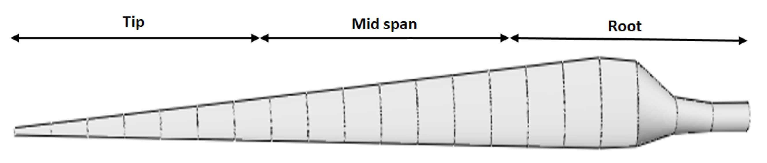
Wind turbines can be categorized, for example, based on their rotation axis, which can be vertical or horizontal [3]. Horizontal axis turbines are the most common and can be classified according to the rotation of the rotor with respect to the tower. These machines are composed of a foundation, a tower, a rotor, nacelle with power train and the blades. The blades are one of the most important components, if not the most, since they are in charge of collecting the energy from the wind, converting the linear movement of the wind into a rotary movement of the rotor. This energy is transmitted to the hub, from the hub it proceeds to a mechanical transmission system and from there it proceeds to the generator that transforms it into electrical energy.

Blades can suffer different types of failures due to a variety of phenomena [4], such as the following: bending, twisting, cracks and erosion. Detecting these types of faults, particularly at early stages, is important for avoiding catastrophic failures, reducing down times and taking corrective actions in a timely manner [5]. In particular, automatically detecting erosion at the leading edge of the blade tip presents a challenge because it is not trivial to properly measure erosion without direct access to the blade [4]. Typically, fault detection in wind turbine blades has been carried out by visual means (https://energy.sandia.gov/programs/renewable-energy/wind-power/, accessed on 29 December 2021), but it is also possible to use different sensor schemes implemented via a SCADA system [5,6]. Afterward, these data can be analyzed by computational models, such as those derived by means of machine learning (ML), which have been found to be of great utility in the detection of damages in a variety of complex scenarios [7,8,9]. One approach of note, for example, is the use of sound to detect such damage [10]. Moreover, to implement ML methods, sufficient data are required to model blades with and without erosion; however, extracting these data from the field or in controlled scenarios can be a complex task to perform [11]; thus, one possible alternative is to exploit simulation software such as QBlade [12].

The goal of this work is two fold. First, it presents a detailed analysis of the effects that erosion has on wind turbine blades, considering modal and numerical analysis, with respect to the physical stress caused by erosion on the blades and the power-generating capacity of a wind turbine. Second, this work presents a methodology to construct ML models that can detect the presence and location of erosion in a blade and measure the amount of erosion as well. The paper makes two important contributions. First, we show for the first time that AutoML can be successfully applied in this problem domain, which has not been considered before for this problem. Second, we show that it is possible to detect the presence of erosion on the blade, determine its location and predict the amount of damage caused by erosion.

The remainder of this paper is organized as follows. Section 2 presents wind turbine blades and the aerodynamic, modal and numerical analysis of the blades studied in this work. Section 3 deals with the detection of erosion with ML methods, including an overview of related works and our experimental approach and results. Finally, conclusions and future work are presented in Section 4.

2. Wind Turbine Blades

During regular operation of a wind turbine blade, air mixed with sand and water droplets will cause severe erosion, which can produce a loss of fatigue resistance of the blade’s surface and cause heavy damage to the blade material, resulting in a loss in electrical potential [13]. Before analyzing the effect of erosion on a wind turbine blade, we first consider the aerodynamic and structural response of the blade caused by erosion.

2.1. Aerodynamic Analysis

Generally, a wind turbine blade is divided in three sections: tip, mid span and root (see Figure 1). These sections are exposed to potential structural damage during normal operation, such as cracks, wrinkles, delamination, debonding and erosion. In particular, this paper is focused on the erosion problem around to the leading edge of the blades. This section presents an analysis of erosion on the blades, identifying the negative effects that erosion has on the power-generating capacity based on power coefficient $C_p$ as well as the power generated by the wind turbine $P_G$.

In order to analyze erosion in a wind turbine blade it is necessary to identify the development of several dynamic parameters, such as the drag coefficient $C_D$, lift coefficient $C_L$ and frequency ${\omega }_n$. For aerodynamic analysis, this study uses the Theory of Momentum (TM), Blade Element Momentum (BEM), Geometry of Blade (GB) and the evaluation of the performance of the wind rotor, considering a case study of a 1 Kw Wind Turbine Generator (WTG). In order to obtain a design as close to the optimum as possible, several aerodynamic surfaces were evaluated to identify suitable conditions of aerodynamic lift based on the pressure gradient of aerodynamics airfoils. The design parameters of the blade and the technical specification of the WTG are provided in

Table 1. Design parameters of the 1 Kw WTG.

Parameter	Value	Variables	Units
Rated power	1000	$P_{\mathrm{nom}}$	W
Number of blades	3	B	[-]
Rated speed	8	$u_{\mathrm{nom}}$	m/s
Speed of rotation	295.63	$\mathsf{\Omega }$	rpm
Gearbox efficiency	0.95	${\eta }_{\mathrm{gearbox}}$	[-]
Generator efficiency	0.95	${\eta }_{\mathrm{gen}}$	[-]
Wind density	1.185	$\rho$	kg/m3
Dynamic Viscosity	1.78 × 10${}^{-5}$	$\mu$	Pa × s

.

For this design, we consider a power coefficient $C_p=0.40$ based on the Betz limit [14], which allows calculating the length (theoretical) of the blade, which results in $R=1.628$[m], and the relationship between the speed and the blade tip in nominal conditions resulting in a value of ${\lambda }_{\mathrm{nom}}\approx 8$. In order to obtain the Reynolds number of the blade, we separate the blade into three sections. We consider an average airfoil in every section of the blade, resulting in the following Reynolds’ numbers. For the root section, the average chord was 0.14 m and Reynolds was 147,000; the average chord of the body is 0.10 m and Reynolds was 198,000, while the average chord of the tip is 0.023 m and Reynolds was 78,000. Finally, BEM parameters used to simulate the blade design were obtained using the method of the Viterna extrapolation [15], which include the following: aspect ratio of 10, lift coefficient adjustment of 0.7 and the number of elements is seven.

Subsequently, from the previous parameters, it is necessary to evaluate several aerodynamics airfoils from databases such as NACA, NREL and WORTMANN. In this work, we evaluated 49 airfoils using the open source QBlade software with the goal of selecting the best and most stable design. The chosen airfoils were FX 63-137 and E216 based on their lift $C_L$ and drag $C_D$ coefficients, both of which influence power coefficient $C_p$ of the turbine.

The designed blade, considering the position of the selected airfoils, chords, spin and Reynolds numbers calculated using QBlade, is show in Figure 2a. The evaluation of aerodynamic performance of the blade using QBlade was carried out using the following parameters: 1 kW of power, an input speed of 3 m/s, cutting speed of 15 m/s, rotor speed of 296 rpm and a density of 1.185 kg/m³. In particular, the work considers the wind conditions of La Ventosa, Oaxaca, Mexico in the Isthmus of Tehuantepec for the simulations, because this geographical zone is located between the Pacific Ocean and the Gulf of Mexico, which is a perfect location for a wind farm [16]. The wind farms are placed near the Pacific Ocean, within a range of 20 and 60 km. In this zone, wind conditions are considered as good (class 4) and excellent (class 7). With a wind speed of 8 m/s, the power generated was 1.38 kW, and the power coefficient was $C_p=0.4197$ with a simulation of 1.4 s.

2.2. Modal Analysis

Structural analysis characterizes the behavior of the blade in the presence of erosion. In particular, this section presents vibration analysis using simulated erosion in the leading edge of the blade tip to compare a clean model with an eroded blade. The material, or mass, loss is expected to cause a variation in the vibration response of the blade, which directly affects the wind rotor and other subsystems of the turbine, such as the gearbox, main shaft and the generator due to the coupling between them. Furthermore, structural analysis is carried out to analyze the response frequency of the blade through modal analysis using a finite element software. This is performed by considering both a clean blade and an eroded version. For structural analysis, the mechanical and physical proprieties of the blade materials are described in

Table 2. (a) Wind turbine blade design. (b) Blades properties.

(a)
Position	Airfoil	Chord
0	Circular Airfoil	0.07
0.077	Circular Airfoil	0.07
0.077	Circular Airfoil	0.07
0.228	E216	0.14
0.46	E216	0.12
0.693	E216	0.11
0.926	E216	0.1
1.158	FX 63-137	0.08
1.391	FX 63-137	0.06
1.6323	FX 63-137	0.023
(b)
Property	Value	Units
Density	2000	(Kg/m3)
Orthotropic elasticity
Young’s Module in x	50,000	MPa
Young’s Module in y	8000	MPa
Young’s Module in z	8000	MPa
Poisson’s ratio $xy$	0.3	-
Poisson’s ratio $yz$	0.4	-
Poisson’s ratio $xz$	0.3	-
Stiffness module $xy$	5000	MPa
Stiffness module $yz$	3846.2	MPa
Stiffness module $xz$	5000	MPa

b. Furthermore, dynamic analysis is also necessary in order to obtain natural frequencies and modal shapes of the blade, which was carried out using the following mesh parameters: quadratic order element, uniform size function, medium center of relevance, fast transition, low smoothness, 732 elements and 1768 nodes.

Simulated erosion was carried out with QBlade considering the tip of the blade, which should effect drag and lift coefficients, as well as the power coefficient and the electric power generated by the turbine. Erosion analysis consist of modifying the geometry of the blade to represent damage on the surface of the tip. The damage due to erosion reduces the original mass of the blade, which is represented in terms of a percentage in profile reduction, as shown in Figure 2b. For this analysis, three different depths of erosion were considered for the bottom edge of the profile, denoted as percentages by $B{I}_1=10\%$, $B{I}_2=18\%$ and $B{I}_3=25\%$. In each case, these percentages represents a reduction in profile coordinates relative to the clean blade. This is shown in Figure 2c, where the black line represents the clean profile, and the blue line represents the eroded profile for the $B{I}_1$ case.

Modal analysis is performed to evaluate the effects of different levels of erosion on the mechanical structure of the blade through their frequency response. The complete results are summarized in

Table 3. Comparative analysis of modal frequencies of the eroded and the clean blades.

Mode	${\mathit{B}\mathit{I}}_1$	${\mathit{B}\mathit{I}}_2$	${\mathit{B}\mathit{I}}_3$	Clean
	(Hz)
1	3.8954	3.2521	3.9509	3.9887
2	15.631	12.874	14.903	14.317
3	23.60	22.268	23.411	22.469
4	42.867	35.699	38.514	38.207

, where four modal frequencies are evaluated for each case of erosion depth compared with the numerical response of the clean blade.

2.3. Numerical Analysis

The drag and lift coefficients, respectively, $C_D$ and $C_L$, are compared for the three levels of erosion and the clean blade in Figure 3a. The change in the original design of the blade causes a variation in the power coefficient $C_P$ and the electric power generated $P_G$.

In order to complete analysis, the lift coefficient $C_L$ is compared with respect to the leading edge of the blade, which is denoted by $\alpha$ using QBlade, as shown in Figure 3b. Parameter $\alpha$ represents the angle of inclination of the blade with respect to the direction of the wind force. This angle can change in a range between −20 to 20 degrees. In this study, the simulation tests were carried out considering $\alpha$ with values of 10 and 20 degrees. For the three erosion cases considered here, $B{I}_1$, $B{I}_2$ and $B{I}_3$, $\alpha$ = 10 degrees. Figure 3b shows the behavior of $C_L$ relative to our three erosion levels. The percentage of erosion on the leading edge of the blade impacts its aerodynamic response, particularly the lift and drag coefficients ($C_L$) and ($C_D$). Figure 3a,b show both coefficients reducing their performance when erosion is increased, this considering a particular angle of attack of 10 degrees. The power coefficient ($C_p$) of the wind rotor is affected by the presence of erosion as well, minimizing the electricity production potential ($P_G$), shown in Figure 3c,d.

Table 4. Comparison of the leading edge in three different erosion’s depth for the drag coefficient $C_d$ and the lift coefficient $C_l$. Last two columns show the percentage difference relative to the clean blade ($C_d$(%) and $C_l$(%)).

Blade	$\mathit{\alpha }$	${\mathit{C}}_{\mathit{d}}$	${\mathit{C}}_{\mathit{l}}$	${\mathit{C}}_{\mathit{d}}$(%)	${\mathit{C}}_{\mathit{l}}$(%)
Clean	10	$0.036$	$1.66$	-	-
$B{I}_1$	10	$0.036$	$1.64$	$0\%$	$1.3\%$
$B{I}_2$	10	$0.03$	$1.46$	$16.7\%$	$13\%$
$B{I}_3$	10	$0.028$	$1.44$	$22.3\%$	$14\%$

presents comparative results of the drag coefficient $C_d$ and the lift coefficient $C_l$ for the three levels of erosion, with respect to the clean blade. Both coefficients are reduced when the depth of the damage is increased on the surface of the blade, affecting aerodynamic performance.

Finally, the behavior of the power coefficient $C_P$ considering $B{I}_1$ is shown in Figure 3c, where the blue line represents the clean blade and the red line represents the eroded blade. It is possible to observe the variation of $C_P$, which decreases to $C_P=0.39$, while $C_P=0.41$ for the clean blade. The power output generated $P_G$ is also affected by erosion, which decreases to around $P_G=1.30$ kW with respect to $P_G=1.36$ kW for the clean blade, as shown in Figure 3d.

2.4. Experimental Modal Analysis

In order to validate our simulated model of erosion, the following tests were carried out using a physical model. The blade was manufactured with a mixture of fiberglass, catalyst and resin. To cause the different levels of erosion on the leading edge of the blade, a Dremel tool was used, which uses a disc to gently sand and abrade the area of interest. Finally, to measure the percentage of erosion, a Vernier was used, measuring depth and thickness at the worn area. The experimental test of the blade was carried out in the Laboratory of Vibration of the Department of Mechatronics Division in the CINVESTAV–IPN. To evaluate the levels of erosion discussed in the numerical results, it was necessary the use an electromagnetic shaker model ET-139 (manufactured by Labworks©) to excite the blade, which is mounted over a mechanical rail supported by a mechanism of ball bearing that allows limited horizontal displacement. The electromagnetic shaker is controlled via a linear power amplifier (manufactured by Labworks©) model PA-138. The response in terms of acceleration and force applied by the electromagnetic shaker to the blade is monitored by using an impedance head placed at the stinger of the shaker connected via a cable to the data acquisition system (manufactured by Klister LabAmp©). The frequency response of the system is fed back using accelerometers model 8640A (manufactured by Klister©) mounted at the tip section of the blade. The data acquisition system is connected via USB to an external graphical interface implemented in MATLAB/Simulink© for the analysis of experimental data captured with a Sensoray© card. A comparative study of the experimental and Finite Element Method (FEM) response (simulation) of a wind turbine blade of 1 Kw of electrical power of the first three vibration modes is summarized

Table 5. Modal analysis of the simulated (FEM) and physical (experimental) blade under different erosion conditions; values given in Hz.

Mode	FEM	Experimental
Level of Erosion $B{I}_1$
1	3.89	3.45
2	15.6	14.6
3	23.6	29.3
Level of Erosion $B{I}_2$
1	3.25	3.5
2	12.8	14.9
3	22.2	29.2
Level of Erosion $B{I}_3$
1	3.95	3.49
2	14.9	14.8
3	23.4	29.0

. Results indicate that our simulated model behaves consistently with the real-world tests. The variations in the frequency response of the blade is due to the loss of material on the leading edge of the tip section, which can compromise the stability and balance of the wind rotor.

3. Erosion Detection with Machine Learning

This section deals with the automatic detection of erosion in wind turbine blades. The goal is to detect where erosion has occurred using a classification model, considering the three different cases of where erosion can appear on the blade tip: on the bottom edge, the top edge or both. Moreover, we predict, using regression models, the amount of erosion on the blade. Both tasks are posed as supervised learning problems and solved using ML algorithms by performing feature extraction on the power and vibration response of the blade through QBlade simulation. However, before presenting our proposal, we briefly survey related works in this domain.

3.1. Related Work

Several works have applied ML towards the detection of different types of problems in wind turbines. For instance, static and dynamic regression models have previously been used to detect failures in wind turbines based on vibration analysis [5]. Another example is [17], which presents an approach to predict when preventive maintenance should be performed, focusing on the remaining useful life of a wind turbine before a failure occurs and diagnosing the type of failure. The proposal involves low implementation costs because it is based solely on information collected from the very common SCADA system. A recent example also includes forecasting of wind speed assessment using satellite data and ML [18], specifically a neural network.

In [11], the authors classify the occurrence of different types of failures in blades, using a piezoelectric accelerometer to measure the vibration of the blade. That work considered five types of damage to the top of the leading edge of the blades, namely bending, cracks, looseness, pitch, twist and erosion. To classify the signals time-domain, feature extraction is performed on the vibration signals, focusing on different types of summary statistics. In a more recent study by the same authors [19], they also use vibration signals, histogram features and ML to monitor the condition of wind turbine blades, in this case using lazy classifiers.

ML has also been applied to maintenance management of blades in [20]. The work is based on the detection of delamination, a common structural problem that can generate large costs. Continuous monitoring of turbines is the focus of [21], using real data from a SCADA system to predict damage to the structure and blades of wind turbines. The authors present two models for this: the first is the use of multilayer neural network, and the second is adaptive networks with a fuzzy inference system. The proposal is to monitor the power curve signal, achieving good precision. Sound analysis, a unique approach, has also been used for fault detection, extracting descriptive feature of acoustic waves and detecting damage using common ML methods [10]. A related work can be found in [22], where ML is used to estimate turbine energy yield losses due to erosion on the leading edge of the blade.

In general, few works deal specifically with erosion, and those that do not focus on a detailed analysis of this type of failure.

3.2. Data Set

The dataset was generated with QBlade and the procedure outlined in Section 2.2. A total of 100 blades were simulated for each type of erosion of the blade tip (bottom edge, top edge or both), producing a dataset with 300 samples, similar to [11]. This work assumes that all blades used in a real-world setting will have a certain amount of erosion in at least one of the edges of the tip. Therefore, we do not consider the case in which the blade is completely clean. It must be stated that, while we are relying on simulated data, it has been shown that simulated results of wind turbine blade performance are reliable predictors of on site behavior [22,23].

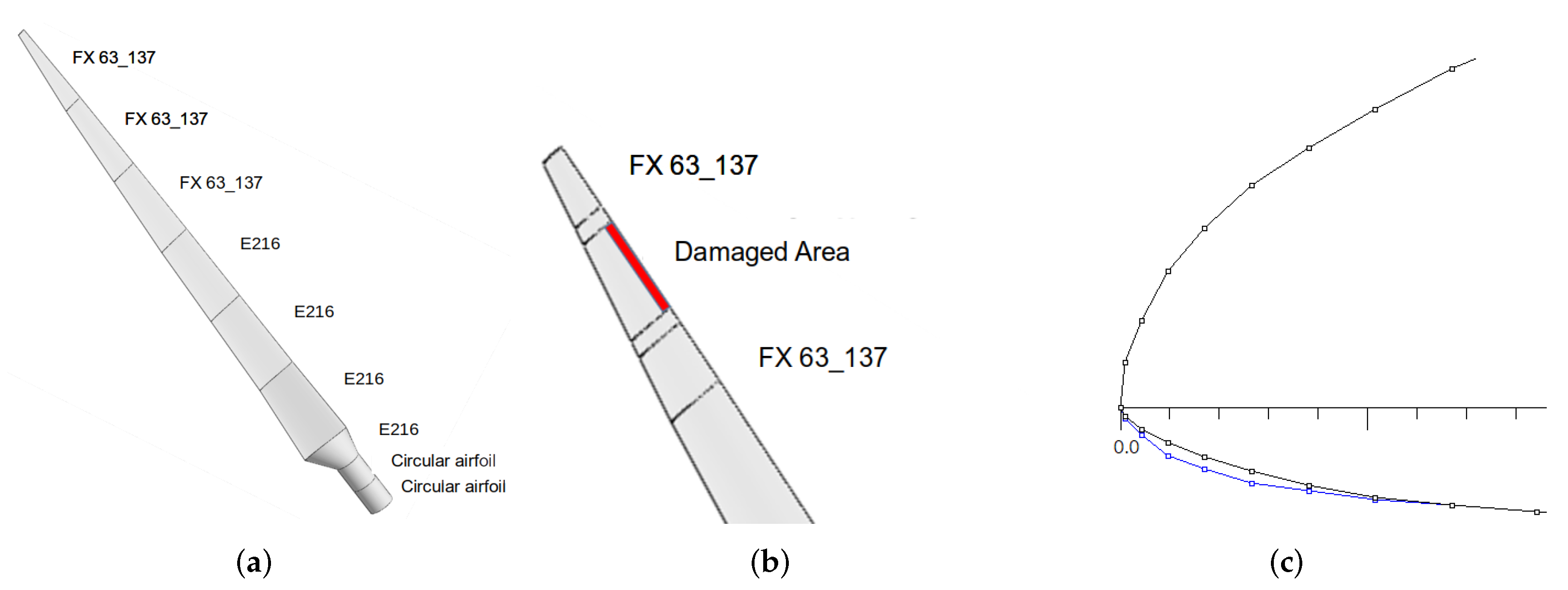
In order to simulate an eroded blade, each of the contour points of the blade profile was perturbed, adding displacements within the range of 8% to 18%. The same seven contour points on the tip of the blade were modified to model different levels of erosion. Half of the samples were generated using uniform grid sampling, while the other half of samples were generated with random values within the specified range. For example, for the lower edge cases, 8% of erosion was removed from the Y-axis coordinate value; subsequently, the percentage of erosion increased by 0.2% up to 18% to generate 50 samples. For the remaining 50 samples, the amount of erosion was determined randomly by using a uniform distribution $U[8,18]$. Random samples were used to simulate a rugged surface on the blade, which can be caused by random events such as contact with insects or large sand particles. Our approach is justified since roughness on a blade is often simulated with a random surface [24,25].

Each blade was simulated with QBlade using the settings in Section 2.1. The acceleration response at the blade tip was obtained, using the QFEM tool for structural design and modal analysis of each blade. The NREL FAST tool [26] was used to carry out analysis of the dynamic response of wind turbines. The vibration of the acceleration signal at the tip of the blade is selected as output. The simulation parameters are as follows: time step of 0.1, 3 blades, a rotor speed of 296 rpm and air density of 1.225 k/m${}^3$. The wind fields are specified in

Table 6. Wind field and wind simulation parameters.

Windfield Parameter	Value
Time (s)	60
Timesteps	100
Point per direction	20
Simulation Parameter	Value
Rotor Radius (m)	30
Hub Height (m)	60
Mean Wind Speed (m/s)	13
Measurement Height (m)	10
Turbulence Intesity (%)	10
Roughness Length (m)	1.00 × ${10}^{-2}$

by mostly using the same simulation values used to determine power output. The difference is simulation time and air density.

3.3. Feature Extraction

After obtaining the samples of both power and acceleration for the different blades, we proceeded to perform feature extraction. For this work, feature detection was carried out in the time domain given the success of such measures in similar work [11] and in the analysis of other complex signals [27,28].

Let $\xi \left(t\right)\in {\mathbb{R}}^T$ denote the vector containing a time series from a single signal, and T denotes the number of samples in $\xi$. A feature of $\xi \left(t\right)$ is denoted by x, while the matrix $\mathbf{X}=[{\mathbf{x}}_1,\dots ,{\mathbf{x}}_F]$ contains all features from all samples, ${\mathbf{x}}_i$ is the vector of a single feature, and F is the total number of features extracted.

The feature extracted from the signals include six statistical descriptors, namely mean, median, maximum, minimum, sum, standard deviation, variance and kurtosis. Moreover, we also extract the following:

• Power: $P_{\xi }=\frac{1}{T}{\mathsf{\Sigma }}_{-\infty }^{\infty }{\left|\xi \left(t\right)\right|}^2$;
• First difference: ${\delta }_{\xi }=\frac{1}{T-1}{\mathsf{\Sigma }}_{t-1}^{T-1}|\xi (t+1)-\xi \left(t\right)|$;
• Normalized first difference: ${\overline{\delta }}_{\xi }=\frac{{\delta }_{\xi }}{{\sigma }_{\xi }}$;
• Second difference: ${\gamma }_{\xi }=\frac{1}{T-2}{\mathsf{\Sigma }}_{t-1}^{T-2}|\xi (t+2)-\xi \left(t\right)|$;
• Normalized second difference: ${\overline{\gamma }}_{\xi }=\frac{{\gamma }_{\xi }}{{\sigma }_{\xi }}$.

Power $P\xi$ measures the strength of the signal or the energy consumed per unit of time. The first and second differences show the changes of a signal in time. The normalized first difference is also known as the Normalized Length Density and is used to quantify the self-similarities contained in a signal. Additionally, we also extract what is referred to as Hjorth features [29]. These include the following: Activity, Mobility and Complexity. The Activity feature represents the variance of the signal and is computed by the following.

$$A_{\xi }=\frac{{\mathsf{\Sigma }}_{t=1}^T{(\xi \left(t\right)-{\mu }_{\xi })}^2}{T}.$$

The Mobility feature is defined by the standard deviation of the slope of the EEG signal using as reference the standard deviation of the amplitude expressed as the following ratio by time unit.

$$M_{\xi }=\sqrt{\frac{var\left(\dot{\xi }\left(t\right)\right)}{var\left(\xi \right(t\left)\right)}}.$$

The Complexity feature measures the signal’s variation using a smooth curve as reference provided by the following.

$$C_{\xi }=\frac{M\left(\dot{\xi }\left(t\right)\right)}{M\left(\xi \right(t\left)\right)}.$$

Another time domain feature is the Non-Stationary Index (NSI) [30]. Signal $\xi$ is divided into segments, and their respective ${\mu }_i$ is computed. NSI is defined as the standard deviation of the segments’ ${\mu }_i$. When NSI is high, the signal is considered to be “less stationary.”

The last feature includes Higher Order Crossings (HOC) [31]. The feature describes the oscillatory nature of signal counting the number of sign changes over multiple variants of the signal. A total of 10 distinct featur HOC features were extracted.

In total, this work considers 27 time domain features to characterize the signals of interest extracted from the wind turbine blade.

Classification and Regression Problems

The above feature extraction process produces a total of 27 time domain features for each signal. These features are used to pose three classifications by using the following: (1) the features from the power signal; and (2) adding the features from the acceleration signal. An ML model will learn to use these features to determine what edge of the blade is affected by erosion.

Moreover, the same feature set will be used to generate a regression model to estimate the exact amount of erosion. In this scenario, the objective is to predict the level of erosion, which ranges from 8 to 18 percent. In this case, the location of the erosion (top, bottom or both) is not taken into account, and the percentage of erosion is the target of the learning process.

3.4. Auto Machine Learning with H2O-DAI

AutoML is an approach for automating the design, tuning, implementation and evaluation of complete ML pipelines. The goal is to simplify the manner in which ML models are tested and evaluated such that the process by which the models are generated provide a comprehensive evaluation of the best possible approach to solve a given problem. In this proposal, we use H2O-DAI, which stands for H2O Driverless AI, which offers a very simple user interface and a comprehensive set of tools to perform AutoML [32]. For instance, it makes a choice from a set of state-of-the-art models, such as XGBoost [33], Generalized Linear Models [34] and Deep Learning [35].

There are basically four tuning hyperparameters that are used to configure the AutoML process of H2O-DAI; these include the following. Accuracy refers to the amount of effort to find the best possible pipeline in the range (1–10); it is set to 7 in these experiments. Time controls the duration of the search process, it is set to 2 in our experiments. Interpretability controls the amount of feature engineering performed by the AutoML system. In this case, since a diverse set of features is already being used, it is set to 8. Moreover, to evaluate performance, 6-fold cross validation was used. All experiments were carried out on an IBMP Power 8 Server for High-Performance Computing with two Power 8 processors and two NVIDIA Tesla P100 GPUs.

3.4.1. Classification Results

Summary of the results are presented as an average confusion matrix based on the classification achieved on the testing folds of the cross validation process. Results are shown in

Table 7. Average confusion matrix using the power signal for feature extraction.

	Bottom	Top	Both	Error
Bottom	99%	1%	0	1%
Top	0	100%	0	0
Both	0	1%	99%	1%

when using the power output for feature extraction, where class labels are shown as Bottom, Top and Both for each of the three types of erosion. Other noteworthy classifier performance scores include (given as the average ± standard deviation over all the testing folds) the following: Area Under the Receiver Operating Characteristic Curve of $0.99\pm 0.001$ and an F1-Score of $0.98\pm 0.008$.

H2O DAI converged to an XGBoost model for classification [36], using a total of seven input features, four of which are raw features from the 27 time domain features and three automatically engineered features. In particular, for this version of the problem, H2O DAI focused on statistical features, such as the variance, mean and median, but it also used the power feature.

Extending the feature set, incorporating the features computed on the acceleration signal produced optimal results, as shown in the confusion matrix of

Table 8. Average confusion matrix using both the power signal and the acceleration signal for feature extraction.

	Bottom	Top	Both	Error
Bottom	100%	0	0	0%
Top	0	100%	0	0
Both	0	0	100%	0

. In this case, H2O DAI also converged to an XGBoost model, using a total of 10 input features, including five automatically engineered features. It is notable that all of the features used in this case are features extracted from the acceleration signal, including the first differential, the NSI and the power features.

3.4.2. Regression Results

The same configuration of H2O DAI is used, which was reported above for classification, with the exception that the scoring function is the root mean squared error (RMSE). Results are presented in

Table 9. Regression results for H2O DAI estimating the percentage of erosion showing the average and standard deviation.

	Power	Acceleration	Both
MAE	0.002 (0.0007)	0.001 (0.0007)	0.0009 (0.0001)
$R^2$	0.98 (0.008)	0.98 (0.012)	0.99 (.0004)
RMSPE	2.8 (0.4)	1.9 (1.14)	0.97(0.14)

, showing the average performance on the test sets of the 6-fold cross validation. H2O DAI was applied on three groups of features: power signal, acceleration signal and both, showing the mean absolute error (MAE), coefficient of determination $R^2$ and the root mean square percentage error loss (RMSPE). In all cases, H2O DAI converged to a Light Gradient Boosting Machine (Light GBM) [37]. Results show that using both signals for feature extraction produced a highly accurate model in terms of both $R^2$ and RMSPE.

4. Concluding Remarks

This study presents an in-depth analysis of the aerodynamic and modal response of an eroded wind turbine blade. Efficiently and effectively detecting erosion on a blade can have substantial impacts in preventative and timely maintenance of wind turbines. Results show that it is possible to accurately determine where the erosion is present on the blade (top edge, bottom edge or both) and to estimate the level of erosion (between 8 and 18 percent). This is accomplished by analyzing the power signal of the wind turbine and the vibrations of the blade tip. A large set of time domain features was extracted, and the modeling process is carried out by using an AutoML system, namely H2O DAI. As such, this study represents the first contribution that tackles both the detection, localization and estimation of erosion level on the leading edge of a blade using ML. Moreover, this work is the first to apply AutoML in this domain. The process of designing the ML pipeline was carried out in an automatic fashion, without hampering performance and requiring very little human intervention in the design process. This could motivate further collaborative and multidisciplinary research between applied ML and wind energy maintenance and production.

The results presented in this work are consistent with those reported by [11,19], with the slight performance difference probably due to working with simulated data in our case, which is nonetheless a good predictor of real-world performance, as shown by [22,23] and partially validated by our experiments with a physical model.

Among both signals that were analyzed, the accelerometer readings seem to be more informative relative to the power signal, based both on the classification (erosion detection) and regression (erosion level estimation) problems, with small but consistent differences. Moreover, the best performance was achieved when both signals are used for feature extraction. It should be possible to use both models to automatically detect the presence and level of erosion in a properly instrumented wind turbine blade. Future work will focus on applying the same experimental procedure in a fully working prototype: first in a wind tunnel and then in the field.

References

1. Kaldellis, J.K.; Zafirakis, D. The wind energy (r) evolution: A short review of a long history. Renew. Energy 2011, 36, 1887–1901. [Google Scholar] [CrossRef]
2. Hernández-Escobedo, Q.; Perea-Moreno, A.J.; Manzano-Agugliaro, F. Wind energy research in Mexico. Renew. Energy 2018, 123, 719–729. [Google Scholar] [CrossRef]
3. Spera, D.A. Wind Turbine Technology: Fundamental Concepts in Wind Turbine Engineering, 2nd ed.; ASME Press: New York, NY, USA, 2009. [Google Scholar]
4. Li, D.; Ho, S.C.M.; Song, G.; Ren, L.; Li, H. A review of damage detection methods for wind turbine blades. Smart Mater. Struct. 2015, 24, 033001. [Google Scholar] [CrossRef]
5. Oliveira, G.; Magalhães, F.; Cunha, Á.; Caetano, E. Vibration-based damage detection in a wind turbine using 1 year of data. Struct. Control Health Monit. 2018, 25, e2238. [Google Scholar] [CrossRef]
6. Blanco Martínez, A. Study and Design of Classification Algorithms for Diagnosis and Prognosis of Failures in Wind Turbines from SCADA Data. Ph.D. Thesis, Universitat de Vic-Universitat Central de Catalunya, Barcelona, Spain, 2018. [Google Scholar]
7. Eftekhar Azam, S.; Rageh, A.; Linzell, D. Damage detection in structural systems utilizing artificial neural networks and proper orthogonal decomposition. Struct. Control Health Monit. 2019, 26, e2288. [Google Scholar] [CrossRef]
8. Tang, Z.; Chen, Z.; Bao, Y.; Li, H. Convolutional neural network-based data anomaly detection method using multiple information for structural health monitoring. Struct. Control Health Monit. 2019, 26, e2296. [Google Scholar] [CrossRef] [Green Version]
9. Gu, J.; Gul, M.; Wu, X. Damage detection under varying temperature using artificial neural networks. Struct. Control Health Monit. 2017, 24, e1998. [Google Scholar] [CrossRef]
10. Krause, T.; Ostermann, J. Damage detection for wind turbine rotor blades using airborne sound. Struct. Control Health Monit. 2020, 27, e2520. [Google Scholar] [CrossRef]
11. Joshuva, A.; Sugumaran, V. Wind turbine blade fault diagnosis using vibration signals through decision tree algorithm. Indian J. Sci. Technol. 2016, 9, 1–7. [Google Scholar] [CrossRef]
12. Alaskari, M.; Abdullah, O.; Majeed, M.H. Analysis of wind turbine using QBlade software. IOP Conf. Ser. Mater. Sci. Eng. 2019, 518, 032020. [Google Scholar] [CrossRef]
13. Du, Y.; Chen, W. Numerical simulation of the wind turbine erosion. In Proceedings of the 3rd International Conference on Material, Mechanical and Manufacturing Engineering (IC3ME 2015), Guangzhou, China, 27–28 June 2015; Atlantis Press: Dordrecht, The Netherlands, 2015. [Google Scholar]
14. Vennell, R. Exceeding the Betz limit with tidal turbines. Renew. Energy 2013, 55, 277–285. [Google Scholar] [CrossRef]
15. Mahmuddin, F.; Klara, S.; Sitepu, H.; Hariyanto, S. Airfoil Lift and Drag Extrapolation with Viterna and Montgomerie Methods. Energy Procedia 2017, 105, 811–816. [Google Scholar] [CrossRef]
16. Elliott, D.; Schwartz, M.; Scott, G.; Haymes, S.; Heimiller, D.; George, R. Wind Energy Resource Atlas of Oaxaca; Technical Report; National Renewable Energy Lab. (NREL): Golden, CO, USA, 2003. [Google Scholar]
17. Zhao, Y.; Li, D.; Dong, A.; Kang, D.; Lv, Q.; Shang, L. Fault prediction and diagnosis of wind turbine generators using SCADA data. Energies 2017, 10, 1210. [Google Scholar] [CrossRef] [Green Version]
18. Majidi Nezhad, M.; Heydari, A.; Pirshayan, E.; Groppi, D.; Astiaso Garcia, D. A novel forecasting model for wind speed assessment using sentinel family satellites images and machine learning method. Renew. Energy 2021, 179, 2198–2211. [Google Scholar] [CrossRef]
19. Joshuva, A.; Sugumaran, V. A lazy learning approach for condition monitoring of wind turbine blade using vibration signals and histogram features. Measurement 2020, 152, 107295. [Google Scholar] [CrossRef]
20. Jimenez, A.; Gómez Muñoz, C.Q.; García Márquez, F.P. Machine Learning for Wind Turbine Blades Maintenance Management. Energies 2017, 11, 13. [Google Scholar] [CrossRef] [Green Version]
21. Morshedizadeh, M. Condition Monitoring of Wind Turbines Using Intelligent Machine Learning Techniques. Master’s Thesis, University of Windsor, Windsor, ON, Canada, 2017. [Google Scholar]
22. Cappugi, L.; Castorrini, A.; Bonfiglioli, A.; Minisci, E.; Campobasso, M.S. Machine learning-enabled prediction of wind turbine energy yield losses due to general blade leading edge erosion. Energy Convers. Manag. 2021, 245, 114567. [Google Scholar] [CrossRef]
23. Wu, G.; Zhang, L.; Yang, K. Development and Validation of Aerodynamic Measurement on a Horizontal Axis Wind Turbine in the Field. Appl. Sci. 2019, 9, 482. [Google Scholar] [CrossRef] [Green Version]
24. Nikolov, I.; Madsen, C. Quantifying Wind Turbine Blade Surface Roughness using Sandpaper Grit Sizes: An Initial Exploration. In Proceedings of the 16th International Joint Conference on Computer Vision, Imaging and Computer Graphics Theory and Applications, Virtual Conference. 8–10 January 2021; SCITEPRESS—Science and Technology Publications: Setúbal, Portugal, 2021. [Google Scholar]
25. David, M. Owner Reports-Airfoil Performance Degradation Due to Roughness and Leading-Edge Erosion, Data and Plots-Raw Data; Technical Report; Pacific Northwest National Lab. (PNNL): Richland, WA, USA, 2020. [Google Scholar]
26. Jonkman, J.M. Modeling of the UAE Wind Turbine for Refinement of FAST_AD; Technical Report; National Renewable Energy Lab.: Golden, CO, USA, 2003. [Google Scholar]
27. Hernández, D.E.; Trujillo, L.; Z-Flores, E.; Villanueva, O.M.; Romo-Fewell, O. Detecting Epilepsy in EEG Signals Using Time, Frequency and Time-Frequency Domain Features. In Computer Science and Engineering—Theory and Applications; Sanchez, M.A., Aguilar, L., Castañón-Puga, M., Rodríguez-Díaz, A., Eds.; Springer International Publishing: Cham, Switzerland, 2018; pp. 167–182. [Google Scholar]
28. Jenke, R.; Peer, A.; Buss, M. Feature Extraction and Selection for Emotion Recognition from EEG. IEEE Trans. Affect. Comput. 2014, 5, 327–339. [Google Scholar] [CrossRef]
29. Hjorth, B. EEG analysis based on time domain properties. Electroencephalogr. Clin. Neurophysiol. 1970, 29, 306–310. [Google Scholar] [CrossRef]
30. Hausdorff, J.; Lertratanakul, A.; Cudkowicz, M.E.; Peterson, A.L.; Kaliton, D.; Goldberger, A.L. Dynamic markers of altered gait rhythm in amyotrophic lateral sclerosis. J. Appl. Physiol. 2000, 88, 2045–2053. [Google Scholar] [CrossRef] [PubMed]
31. Petrantonakis, P.C.; Hadjileontiadis, L.J. Emotion Recognition From EEG Using Higher Order Crossings. IEEE Trans. Inf. Technol. Biomed. 2010, 14, 186–197. [Google Scholar] [CrossRef] [PubMed]
32. Hall, P.; Kurka, M.; Bartz, A. Using H2O Driverless AI. Mountain View, CA, USA. 2018. Available online: http://docs.H2O.ai (accessed on 29 December 2021).
33. Zheng, H.; Yuan, J.; Chen, L. Short-term load forecasting using EMD-LSTM neural networks with a Xgboost algorithm for feature importance evaluation. Energies 2017, 10, 1168. [Google Scholar] [CrossRef] [Green Version]
34. Freebury, G.; Musial, W. Determining equivalent damage loading for full-scale wind turbine blade fatigue tests. In Proceedings of the 2000 Asme Wind Energy Symposium, Reno, NV, USA, 10–13 January 2000; p. 50. [Google Scholar]
35. Stetco, A.; Dinmohammadi, F.; Zhao, X.; Robu, V.; Flynn, D.; Barnes, M.; Keane, J.; Nenadic, G. Machine learning methods for wind turbine condition monitoring: A review. Renew. Energy 2019, 133, 620–635. [Google Scholar] [CrossRef]
36. Chen, T.; Guestrin, C. XGBoost: A Scalable Tree Boosting System. In Proceedings of the 22nd ACM SIGKDD International Conference on Knowledge Discovery and Data Mining, San Francisco, CA, USA, 13–17 August 2016; Association for Computing Machinery: New York, NY, USA, 2016; pp. 785–794. [Google Scholar]
37. Ke, G.; Meng, Q.; Finley, T.; Wang, T.; Chen, W.; Ma, W.; Ye, Q.; Liu, T.Y. Lightgbm: A highly efficient gradient boosting decision tree. Adv. Neural Inf. Process. Syst. 2017, 30, 3146–3154. [Google Scholar]
Figure 1. Sections of a wind turbine blade.
Mca 27 00005 g001
Figure 2. (a) Wind turbine blade design. (b) Area of erosion damage. (c) Blue line represents the clean Airfoil FX 63_137, while the dark line is the eroded blade considering case B I 1 .
Mca 27 00005 g002
Figure 3. (a) Relationship between the drag coefficient ( C D ) and the lift coefficient ( C L ). (b) Lift coefficient C L Vs angle of attack α . (c) Power coefficient C p for B I 1 and the clean wind turbine blade. (d) Power output P G for B I 1 and the clean blade.
Mca 27 00005 g003