Article

Multi-Physics Inverse Homogenization for the Design of Innovative Cellular Materials: Application to Thermo-Elastic Problems

1
Dipartimento di Meccanica, Politecnico di Milano, Via La Masa 1, I-20156 Milano, Italy
2
MOX, Dipartimento di Matematica, Politecnico di Milano, Piazza L. da Vinci 32, I-20133 Milano, Italy
*
Authors to whom correspondence should be addressed.
Math. Comput. Appl. 2022, 27(1), 15; https://doi.org/10.3390/mca27010015
Submission received: 7 January 2022 / Revised: 8 February 2022 / Accepted: 9 February 2022 / Published: 15 February 2022
(This article belongs to the Special Issue Computational Methods for Coupled Problems in Science and Engineering)

Abstract

:
We present a new algorithm to design lightweight cellular materials with required properties in a multi-physics context. In particular, we focus on a thermo-elastic setting by promoting the design of unit cells characterized both by an isotropic and an anisotropic behavior with respect to mechanical and thermal requirements. The proposed procedure generalizes the microSIMPATY algorithm to a thermo-elastic framework by preserving all the good properties of the reference design methodology. The resulting layouts exhibit non-standard topologies and are characterized by very sharp contours, thus limiting the post-processing before manufacturing. The new cellular materials are compared with the state-of-art in engineering practice in terms of thermo-elastic properties, thus highlighting the good performance of the new layouts which, in some cases, outperform the consolidated choices.

1. Introduction

Cellular materials represent an effective solution for structural applications where conventional monolithic materials fail to satisfy the design constraints [1]. The fast advancements in additive manufacturing technologies experienced in the last few years have further amplified the interest toward metamaterials. In addition, the possibility to employ a large variety of bulk materials in manufacturing processes (e.g., metals, polymers, ceramics [2,3,4]) has enabled the design of new metamaterials, featuring innovative combinations of physical effective properties. The possibility to blend different materials in order to reach diverse objectives proved to have a great impact in all the contexts where multi-functionality is required. For example, in [5,6,7,8], biocompatible 3D-printed metal bone implants promoting bone ingrowth are proposed by properly tailoring the material microstructure in order to reproduce the elastic modulus and the permeability of the human bone. Other applications range from thermal-cloaking systems fitly combining microstructure geometry and orientation [9,10] to lattice-based heat exchangers, where good thermal conductivity and convection properties are exploited to enhance the devices’ performance [11,12].
From a modeling viewpoint, the proposal of innovative multifunctional cellular materials can benefit from the most recent advancements in topology optimization [13], properly combined with direct and inverse homogenization processes [14,15,16]. Several optimization approaches can be exploited in the context of metamaterial design. The layout of the employed microstructures can be selected a priori, starting from consolidated dictionaries of unit cells [16,17,18,19,20,21], or designed from scratch to match the expected effective properties [22,23,24,25,26,27,28]. In this context, a single- or a multi-objective topology optimization at the microscale can drive the design of new unit cells matching target properties at the macroscale, potentially in a multi-physics framework. For instance, the optimization of homogenized elastic properties is tackled in [29,30,31] with the aim of maximizing the bulk (or shear) modulus. To this aim, the authors control specific components of the homogenized elastic tensor or resort to the minimization of the compliance of a given structural part. Other works focus on a multi-physics optimization (for instance, by considering elastic, thermal, and electrical properties) by providing microstructures optimized with respect to diverse objectives and physics [32,33,34,35].
Nevertheless, it is well-known that standard topology optimization techniques suffer from typical issues that may compromise the effective performance and manufacturability of the new layouts. Among the most recurrent, we mention the possible presence of intermediate densities, the non-smooth contours of the final design and the generation of unit cells which turn out to be unprintable since presenting too thin struts. All these drawbacks are strictly related to the selected computational grid: a coarse mesh promotes jagged boundaries and a diffused void/material interface; vice versa, an extremely fine mesh leads to a non-affordable computational effort and fosters the generation of too complex structures. Filtering offers a possible remedy to address all these concerns by alternating smoothing with sharpening phases to be properly tuned. Such a tuning is not a trivial task and may often lead to non-optimal design solutions [13,33,36].
The selection of a computational mesh customized to the design problem has been proved to be instrumental in order to limit the main issues of topology optimization. For instance, in [37], the combination of a standard density-based method for topology optimization with an anisotropic mesh adaptation procedure has been used to get rid of intermediate densities, irregular boundaries, and thin struts in the design of structures at the macroscale. The proposed algorithm, named SIMPATY (SIMP with mesh AdaptiviTY), is based on a robust mathematical tool, namely an a posteriori estimator for the discretization error, and it leads to final designs characterized by reliable mechanical properties as well as by free-form features. The same procedure has been successfully exploited at the microscale, with the proposal of the microSIMPATY algorithm [26]. So far, this procedure has been used for the design of unit cells with optimized mechanical properties in a linear elasticity setting [27,38].
In this work, we propose a new pipeline for the design of new cellular materials by extending the microSIMPATY algorithm to a multi-physics context. The objective is to obtain lightweight metamaterials with prescribed requirements on the elastic and thermal conductivity properties, which are characterized by a ready-to-print topology. The design strategy here developed is confined to a 2D setting and has to be meant as a proof-of-concept, preliminary to a 3D implementation. However, to corroborate the effectiveness of the proposed methodology, we perform a cross-comparison between the new cells and the standard ones in thermo-elastic applications.
The paper is organized as follows. Section 2 represents the core of the paper. It provides the physical problem constraining the optimization process, outlines the main theoretical tools to perform the optimization, and formalizes the thermo-elastic design procedure in the MultiP-microSIMPATY algorithm. Three design cases are considered in Section 3 to apply the MultiP-microSIMPATY algorithm to diverse scenarios. Section 4 further analyzes the results in the previous section by comparing the new designs with the state-of-the-art. Finally, Section 5 outlines the most remarkable contributions of the work together with some future perspectives.

2. Methods

In this paper, we refer to a multi-physics framework, in order to provide new layouts for the design of cellular materials. A standard issue consists in optimizing the microscale to ensure desired properties at the macroscale. To deal with this two-scale setting, it is crucial to properly transfer the physical characterization of the micro- to the macroscale. Direct and inverse homogenization represent widespread solutions in such a direction [14,39,40,41]. In particular, the direct approach incorporates the microscopic effects into a homogenized macroscopic model. As a consequence, the microscopic behavior is known, whereas we have to identify the (homogenized) macroscopic characterization. Vice versa, inverse homogenization starts from desired macroscopic physical properties and designs the microscale in order to match such features, thus swapping the role played by known and unknown scales with respect to direct homogenization.
In this paper, we focus on a two-dimensional setting and on linear thermo-elastic properties, so that, at the macroscale, the reference models are the linear elasticity equation [42] and the linear thermal conduction problem, as identified by the standard stress–strain ( σ - ε ) and heat flux-temperature ( q - θ ) relations, given by
σ ( u ) = σ 11 ( u ) σ 22 ( u ) σ 12 ( u ) = E 1111 E 1122 E 1112 E 2211 E 2222 E 2212 E 1211 E 1222 E 1212 ε 11 ( u ) ε 22 ( u ) 2 ε 12 ( u ) = E ε ( u ) ,
and
q ( θ ) = q 1 ( θ ) q 2 ( θ ) = k 11 k 12 k 21 k 22 θ x 1 θ x 2 = k θ ,
respectively, where E and k are the stiffness and the conductivity tensors characterizing the considered solid material.
We observe that in view of the homogenization procedures, the constitutive laws (1) and (2) have to be properly modified to include the effects of the microscale, into
σ H ( u ) = E H ε ( u ) , q H ( θ ) = k H θ ,
where E H and k H denote the homogenized stiffness and thermal conductivity tensors, as detailed in the next section.

2.1. Inverse Homogenization

Inverse homogenization is the procedure that allows us to design microstructures with prescribed properties at the macroscale. The required features are mathematically commuted into a goal functional J and into suitable constraints driving a topology optimization process to be solved in the unit cell Y R 2 whose periodic repetition yields the cellular material  [26,27,29,38,43]. According to a density-based approach, a standard way to perform such an optimization leads us to define an auxiliary scalar field, ρ , that models the relative material density at the microscale. A priori, it is assumed that ρ = 1 labels the material, while ρ = 0 identifies the void. However, since density ρ L Y , [ 0 , 1 ] can take all the values in [ 0 , 1 ] , it is standard to penalize the intermediate values (i.e., intermediate material densities) that are not physically consistent. To this aim, we resort to the SIMP method, which modifies the reference state equations by weighting the constitutive laws with a suitable power of the density [13].
In general, the optimization problem we are interested to solve is
min ρ L Y , [ 0 , 1 ] J ( z ( ρ ) , ρ ) : a ρ z ( ρ ) , w = F ρ ( w ) w W L B C ( z ( ρ ) , ρ ) U B ,
where z = z ( ρ ) denotes the state variable depending on the density field, a ρ ( · , · ) together with F ρ ( · ) defines the state equation constraining the topology optimization, W is a suitable function space [44], and the box inequality includes specific design and physical requirements, with C ( · , · ) being the vector gathering the quantities to be controlled through the corresponding lower and upper bounds, L B a U B .
In the analysis below, we pick the objective functional J as
M ( ρ ) = Y ρ d Y
since we are interested in minimizing the total mass, M , of the cellular structure, i.e., to design lightweight materials.
According to a standard homogenization procedure, as the state equation, we select the linear elasticity model at the microscale weighed by the density function, which describes the Y-periodic displacement field fluctuations, u * , i j , induced by the test displacement fields u 0 , i j , with u 0 , 11 = [ x , 0 ] T , u 0 , 22 = [ 0 , y ] T and u 0 , 12 = [ y , 0 ] T . This leads us to identify the forms a ρ ( · , · ) and F ρ ( · ) in (3) with
a ρ E , i j u * , i j ( ρ ) , v = 1 | Y | Y ρ p σ ( u * , i j ) : ε ( v ) d Y , F ρ E , i j ( v ) = 1 | Y | Y ρ p σ ( u 0 , i j ) : ε ( v ) d Y ,
respectively, with p R + , i j I = { 11 , 22 , 12 } , and where the superscript E refers to the elasticity setting. The state equation associated with (5) is completed with fully periodic conditions on the cell boundary Y , according to the asymptotic homogenization theory. Thus, W in (3) coincides with the space U # 2 = [ H 1 ( Y ) ] 2 of the H 1 ( Y ) -vector functions satisfying periodic boundary conditions along Y .
To include also the thermal component in the topology optimization, we further constrain the process with the ρ -weighed thermal conductivity model at the microscale, which are characterized by the forms
a ρ k , m ( θ * , m ( ρ ) , v ) = 1 | Y | Y ρ s q ( θ * , m ) : v d Y , F ρ k , m ( v ) = 1 | Y | Y ρ s q ( θ 0 , m ) : v d Y ,
with s R + , m J = { 1 , 2 } , and where the superscript k refers to the thermal framework. Analogously to (5), we complete the thermal state equation identified by (6) with periodic boundary conditions along Y , so that θ * , m and v U # 1 = H 1 ( Y ) , where θ * , m denotes the temperature fluctuations associated with the test temperature fields θ 0 , m (namely, θ 0 , 1 = x and θ 0 , 2 = y ).
The two problems at the microscale, (5) and (6), are instrumental to define the homogenized elastic tensor, E H , and the homogenized thermal conductivity tensor, k H , which will be involved in the box constraints in (3). The component-wise definition of E H and k H is
E i j k l H = 1 | Y | Y ρ p σ ( u 0 , i j ) σ ( u * , i j ( ρ ) ) : ε ( u 0 , k l ) ε ( u * , k l ( ρ ) ) d Y ,
k m n H = 1 | Y | Y ρ s q ( θ 0 , m ) q ( θ * , m ( ρ ) ) : θ 0 , n θ * , n ( ρ ) d Y ,
respectively, with i j , k l I and m , n J . In particular, the two-sided inequality in (3) will be exploited to promote diverse mechanical and thermal behaviors along the different spatial directions. To this aim, we constrain the two ratios E 2222 H / E 1111 H and k 22 H / k 11 H so that they vary in suitable ranges. This choice allows us to penalize the mechanical and the thermal contributions in a different way along the two directions, as shown in the numerical assessment. An additional two-sided control is enforced on the first and the last diagonal terms, E 1111 H and E 1212 H , of the homogenized elastic tensor, as well as on the first diagonal term, k 11 H , of the homogenized thermal conductivity tensor.
To sum up, the optimization setting we are led to deal with coincides with the following problem:
min ρ L Y , [ 0 , 1 ] M ( ρ ) : a ρ E , i j u * , i j ( ρ ) , v = F ρ E , i j ( v ) v U # 2 , i j I a ρ k , m θ * , m ( ρ ) , v = F ρ k , m ( v ) v U # 1 , m J E 1111 low E 1111 H E 1111 up E 1212 low E 1212 H E 1212 up E 2222 E 1111 low E 2222 H E 1111 H E 2222 E 1111 up k 11 low k 11 H k 11 up k 22 k 11 low k 22 H k 11 H k 22 k 11 up ρ min ρ 1
where all the bound values, ( · ) low and ( · ) up , will be set according to the application at hand and in order to avoid an unfeasible solution (inappropriate constraints might lead to an empty solution space). Finally, the last inequality in (9) is meant to ensure the well-posedness of both the elasticity and the thermal problems (5) and (6), ρ min being a suitable value in ( 0 , 1 ) (see Section 3 for more details).

2.2. Discretization on Anisotropic Adapted Meshes

With a view to the solution of problem (9), all the quantities involved in the state equations, as well as in the constraints, have to be discretized on a suitable tessellation of the unit cell Y. For this purpose, we resort to a computational mesh T h = { K } customized to the problem at hand and characterized by stretched elements (i.e., a so-called anisotropic adapted mesh). Mesh T h is employed to discretize both the test and the trial functions in the state equations, as well as the density function ρ , by means of a finite element scheme [44].
The anisotropic reference setting is the one proposed in [45]. In particular, the anisotropic features of each element K coincide with the lengths, λ 1 , K , λ 2 , K , and the directions, r 1 , K , r 2 , K , of the semi-axes of the ellipse circumscribed to K through the standard affine map, T K : K ^ K , between the reference element K ^ and the triangle K.
Concerning the adaptation procedure, we resort to a metric-based approach driven by an a posteriori estimator for the discretization error associated with the density function ρ . Among the error estimators available in the literature [46,47], we refer to an a posteriori recovery-based error analysis. Following the seminal work by O.C. Zienkewicz and J.Z. Zhu [48], we control the H 1 -seminorm of the discretization error on the density, e ρ = ρ ρ h . The selection of such an estimator is motivated by the fact that the density ρ exhibits strong gradients (i.e., large values for the H 1 -seminorm) across the material–void interface. This feature will yield meshes whose elements are crowded along the boundaries of the structure, thus promoting the design of very smooth layouts. To this aim, we exactly integrate the so-called recovered error, E = P ρ h ρ h , namely,
| e ρ | H 1 ( Y ) 2 = e ρ L 2 ( Y ) 2 = Y | ρ ρ h | 2 d Y E L 2 ( Y ) 2 = Y | P ρ h ρ h | 2 d Y ,
where ρ h denotes the finite element discretization of ρ in the space V h r of the piecewise polynomials of degree r N associated with T h . The operator P : [ V h r 1 ] 2 [ V h s ] 2 in (10), with s N , denotes the recovered gradient, which, in general, provides a more accurate estimate of the exact gradient ρ with respect to the discrete gradient ρ h . Several recipes are available in the literature to define P [49,50,51,52]. In particular, we select operator P : [ V h 0 ] 2 [ V h 0 ] 2 as the area-weighted average of ρ h over the patch of the elements, Δ K = { T T h : T K } , associated with K; i.e., we opt for
P ρ h ( x ) = 1 | Δ K | T Δ K | T | ρ h | T x K ,
with | ω | the area of the generic domain ω R 2 , where we have set the degree of the finite element space for ρ h to r = 1 . Space V h 1 is also adopted to discretize the components of the displacement vectors u * , i j as well as the temperature fields θ * , m in (9), with i j I and m J .
According to [53,54], we here adopt the anisotropic generalization of (10). This estimator essentially exploits the anisotropic counterpart of the definition of the H 1 -seminorm [45], based on the symmetric semidefinite positive matrix G Δ K , with entries
G Δ K ( g ) i , j = T Δ K T g x i g x j d T i , j = 1 , 2 ,
with g H 1 ( Y ) , and where it is understood x 1 = x and x 2 = y . Thus, the squared H 1 -seminorm | e ρ | H 1 ( Y ) 2 is evaluated by the (global) error estimator η 2 = K T h η K 2 , where
η K 2 = 1 λ 1 , K λ 2 , K i = 1 2 λ i , K 2 r i , K T G Δ K ( E ) r i , K ,
defines the local error estimator. The contribution between brackets coincides with the projection of the squared L 2 -norm of the recovered error along the anisotropic directions, while the scaling factor ( λ 1 , K λ 2 , K ) 1 guarantees the consistency with the isotropic case (for more details, see [53]).
The new adapted mesh is generated after commuting the error estimator η K into a new mesh spacing (the metric), M , consisting of the triplet { λ 1 , K a d a p t , λ 2 , K a d a p t , r 1 , K a d a p t } , where the direction r 2 , K a d a p t is automatically defined being r 1 , K a d a p t · r 2 , K a d a p t = 0 , for each element K T h . This operation is performed by taking into account three different criteria, namely, (i) the minimization of the mesh cardinality # T h ; (ii) an accuracy requirement on the discretization error | e ρ | H 1 ( Y ) (i.e, on the error estimator η ), controlled up to a user-defined tolerance TOL; (iii) the equidistribution of the error throughout the mesh elements (i.e., η K 2 = TOL 2 / # T h ). These three criteria lead us to solve a constrained minimization problem on each triangle K T h . The solution to this local optimization problem can be analytically derived, as proved in [55], being
λ 1 , K a d a p t = g 2 1 / 2 TOL 2 2 # T h | Δ ^ K | 1 / 2 , r 1 , K a d a p t = g 2 , λ 2 , K a d a p t = g 1 1 / 2 TOL 2 2 # T h | Δ ^ K | 1 / 2 , r 2 , K a d a p t = g 1
where g 1 , g 2 and g 1 , g 2 are the eigenvalues and the eigenvectors of the scaled matrix G ^ Δ K ( E ) = G Δ K ( E ) / | Δ K | , with g 1 g 2 > 0 .
Finally, the metric M = { λ 1 , K a d a p t , λ 2 , K a d a p t , r 1 , K a d a p t } K T h has to be changed into a quantity associated with the vertices of T h received as an input by the selected mesh generator. A standard choice consists in an arithmetic mean formula applied to the patch of elements associated with each vertex in T h  [54].
The anisotropic mesh adaptation based on the metric (14) is customized to a topology optimization problem in the algorithm SIMPATY, proposed in [37]. This procedure has been successfully employed for the design of structures at the macroscale [37,56,57] as well as for the design of new metamaterials with the proposal of the algorithm microSIMPATY [26,27]. Moreover, a combination of topology optimization at the macroscale and at the microscale is carried out in [38]. In particular, a multiscale topology optimization process is used for the design of orthotic devices for 3D printing manufacturing with the proposal of patient-specific innovative solutions.
It has been verified that the adoption of an adapted anisotropic mesh leads to free-form layouts characterized by very smooth boundaries both at the macroscale and at the microscale, mitigating some of the well-known drawbacks of standard topology optimization, such as the massive employment of filtering, the staircase effect, and the generation of too complex structures [13,33,36]. However, in [57], it has been observed that the presence of deformed elements inside the structures makes the finite element analysis less reliable. To overcome this issue, the authors suggest a hybrid approach. Thus, the mesh is kept isotropic, with a uniform diameter h iso in the full-material regions, { x Y : ρ h ( x ) > ρ th } with ρ th as a user-defined threshold, whereas the stretched triangles are preserved along the material–void interface. Actually, these hybrid meshes ensure an effective balance between the smoothness of the structure and robust engineering performances (the interested reader can find a quantitative investigation of the benefits of the hybrid approach in terms of accuracy in (Section 5, [57])). For this reason, we resort to hybrid meshes in the sequel.

2.3. Multi-Physics Optimization Algorithm

In this section we propose the multi-physics adaptive inverse homogenization procedure, which generalizes the algorithm proposed in [26]. The discretization of the state equations associated with (5) and (6) is performed with the open-source finite element solver FreeFEM [58], which provides the ideal environment to implement an anisotropic mesh adaptation procedure in Section 2.2 through the built-in mesh generator BAMG (Bidimensional Anisotropic Mesh Generator).
The developed multi-physics optimization procedure is listed in the pseudocode in Algorithm 1. The main loop (lines 3–12) includes an optimization step, a filtering phase, and the mesh adaptation. At each global iteration k, the optimization problem is solved (line 4, function optimize ) by taking into account all the constraints on the components of the elastic and of the thermal conductivity tensors in (9). To this aim, we use the interior point algorithm IPOPT [59], although any other optimization tool can be selected [60]. IPOPT requires as input the functional J to be minimized; the vector C gathering the constrained quantities in the optimization procedure; the two vectors c l and c u of the lower and upper bounds for the components in C ; the array G collecting the derivative of the functional J and of the constraints C with respect to ρ , computed by the adjoint Lagrangian approach (for more details, we refer to [27]); the initial guess ρ h k to start the optimization process; the accuracy TOPT for the minimization problem; the maximum number of iterations IT to stop the optimization. In particular, in the numerical assessment of Section 3, we set TOPT = 10 5 , and IT = 100 for k = 0 and IT = 10 for all the successive iterations. The higher value for IT for k = 0 takes into account that the initial guess ρ h 0 can be completely arbitrary with respect to the minimum to be reached. On the contrary, a smaller value for IT is sufficient for k > 0 , since the initial guess, ρ h k , coincides with the output of a previous optimization step.
Algorithm 1 MultiP-microSIMPATY
1:
Input: CTOL, kmax, c l , c u , ρ h 0 , TOPT, IT, kfmax, τ , β , T h 0 , TOL, HYB
2:
Set: k = 0, errC = 1+CTOL;
3:
while errC > CTOL & k< kmax do
4:
     ρ h k + 1 = optimize( J , C , c l , c u , G , ρ h k , TOPT, IT);
5:
    if  k < kfmax  then
6:
         ρ h k + 1 = helmholtz( ρ h k + 1 , τ );
7:
         ρ h k + 1 = heaviside( ρ h k + 1 , β );
8:
    end if
9:
     T h k + 1 = adapt( T h k , ρ h k + 1 ,TOL, HYB );
10:
    errC = | # T h k + 1 # T h k | / # T h k ;
11:
    k = k+1;
12:
end while
13:
T h = T h k ;
14:
ρ h = ρ h k ;
15:
E H , k H = homogenize( ρ h );
16:
return  T h , ρ h , E H , k H
Function optimize returns the density ρ h k + 1 , which is successively processed by means of Helmholtz and Heaviside filters (lines 6–7, functions helmholtz and heaviside ) [61,62]. The two filtering operations work in a complementary way. The Helmholtz partial differential equation is instrumental to remove too thin features, although promoting intermediate densities along the layout contour. In more detail, it consists of a low-pass filter based on a diffusion kernel with radius τ R + . On the contrary, the Heaviside filter, coinciding with a β -dependent regularization of the Heaviside function with β R + , penalizes the intermediate material densities, also due to the Helmholtz filter, thus increasing the sharpness of the material/void interface. The combined filtering takes place for the first kfmax global iterations only. This choice leads to start the mesh adaptation procedure with a density field, which is free from too complex features, while exhibiting a clear alternation between void and material. The filtering phase becomes redundant when the optimization loop approaches the minimum, so that mesh adaptation alone suffices to ensure well-defined structures. In the next section, filtering parameters τ and β are set equal to 0.02 and 5 respectively, while kfmax = 25 .
The next step coincides with the mesh adaptation procedure detailed in Section 2.2 and here represented by function adapt (line 9). The input parameter TOL establishes the accuracy of the error estimator η through the predicted metric in (14). Parameter HYB is a boolean flag that, in correspondence with the full material, switches the employment of an isotropic mesh on or off.
The main loop is controlled by a check on the stagnation of the relative difference between the cardinality of two consecutive meshes (line 10), up to a maximum number of global iterations kmax (line 3). The choices TOL  = 10 5 and kmax = 100 are preserved throughout all the numerical assessment below.
Algorithm MultiP-microSIMPATY returns the final adapted mesh T h , the optimized density ρ h , and the homogenized elastic and conductivity tensors, E H and k H , which are computed by function homogenize (line 15), based on (7) and (8).
We remark that the procedure itemized in Algorithm 1 is fully general and it can be applied in a straightforward way to different multi-physics contexts after properly modifying the formulation in (9).

3. Results

We analyze three different cases of microstructure design according to (9). In order to highlight the interplay between the different (thermal and mechanical) physics involved, we consider configurations where the thermal conductivity and the elastic stiffness requirements act along different directions. For instance, a high shear stiffness combined with a high thermal conductivity along the x-direction orient the material along two opposite directions, with the prescription of a conflict configuration.
The whole verification below shares common choices for some physical quantities and discretization parameters. In particular, the unit cell Y R 2 is identified with the unitary square, Y = ( 0 , 1 ) 2 . Moreover, we set the Young modulus, E Y , and the Poisson ratio, ν , to 1 and 0.3 , respectively, and we consider an isotropic solid material with unitary thermal conductivity by setting k 11 = k 22 = 1 and k 12 = k 21 = 0 . These choices allow us to obtain normalized homogenized mechanical and thermal properties for the cellular structures. Following [26], both the SIMP-powers, p and s, in (7) and (8) are chosen equal to 4 to penalize intermediate densities.
Concerning the discretization frame, we choose a random density field, ρ h 0 , as the initial guess for the optimization process, in order to avoid any bias. In particular, ρ h 0 is defined on an initial structured mesh characterized by 30 subdivisions per side, and with values ranging from ρ m i n = 10 4 to 1 (see Figure 1 for an example).
Finally, to ensure a reliable finite element analysis, we resort to the hybrid mesh adaptation procedure ( HYB = 1 in function adapt ). In particular, we choose the threshold value ρ th = 0.9 to manage the alternation between isotropic and anisotropic elements, and the isotropic tessellation is characterized by the uniform diameter h iso = 0.03 (approximately 1 / 30 of the design domain dimension).
After the optimization, we perform a verification step to check the actual mechanical and thermal properties of the material yielded by a periodic repetition of the optimized unit cell. To this aim, we use the Abaqus software (Abaqus, Dassault Systèmes Simulia Corp, Johnston, RI, USA). The layouts provided by Algorithm 1 are imported in Abaqus after a thresholding, which neglects the density smaller than 0.75. The obtained geometry is remeshed on a uniform isotropic triangular mesh with an average size equal to 0.01 , while the displacement and temperature fields are discretized with quadratic finite elements, completed with periodic boundary conditions. The verification here performed can be considered as a preliminary step toward the integration of the MultiP-microSIMPATY algorithm into a common workflow for structural analysis.

3.1. Design Case 1

The main goal of this first optimization process is to design a lightweight unit cell characterized by isotropic mechanical homogenized properties and, vice versa, anisotropic thermal homogenized features. This problem can be cast in setting (9), after making the following choices for the constraints:
0.05 E 1111 H 0.08 0.055 E 1212 H 0.080 1 E 2222 H E 1111 H 2 0.01 k 11 H 1.00 0.00 k 22 H k 11 H 0.58 .
The isotropic mechanical behavior and the anisotropic thermal properties are enforced by the constraints in (15) 3 and (15) 5 . In particular, we expect ratios E 2222 H / E 1111 H and k 22 H / k 11 H to coincide with the corresponding lower and upper bounds, respectively. Moreover, since a control on the ratios does not ensure E 1111 H , E 2222 H , k 11 H , and k 22 H to be in a physically admissible range of values, we further constrain the optimization through the box inequalities (15) 1 and (15) 4 . Finally, a control on the component E 1212 H of the homogenized stiffness tensor closes the minimization problem, thus further restricting the solution space.
For the values set for the input parameters, the MultiP-microSIMPATY algorithm converges in 51 global iterations. Figure 2 shows the layout and the associated anisotropic adapted mesh at three different iterations.
We remark that the final topology of the layout is already detected at the first iteration, although the quality of the solution is improved throughout the optimization process. In particular, at the first iteration ( k = 1 ), we observe a significant staircase effect together with the presence of intermediate densities along the microstructure interface. At the end of the filtering phase ( k = 24 ), the jagged boundaries are fully smoothed, despite the intermediate densities still blurring the design. The spreading effect along the material/void interface is gradually reduced when switching off the filtering, i.e., for k > 24 , as shown by the last column in Figure 2. Thus, the final optimized solution ( k = 51 ) shows an extremely sharp transition from material to void and smooth boundaries, which make the structure ready for printing or manufacturing, with a limited need for post-processing.
Concerning the adapted mesh, we recognize the effect of the hybrid approach, which combines stretched elements to discretize the strong gradients of the density field, coarse anisotropic triangles outside the structure, and isotropic elements in correspondence with the material.
Additional quantitative information on the MultiP-microSIMPATY algorithm is provided by Table 1 and by the diagrams in Figure 3, which show the evolution of the objective function and of the constrained quantities (top), together with the trend of the mesh cardinality (bottom), over the global iterations. Notice that the values of the constraints have been normalized between 0 and 1 (see the highlighted area in the top panel of Figure 3). It is evident that the mass exhibits a completely different trend when compared with the constrained quantities. The value of the objective function oscillates with values between 0.325 and 0.475 over the first 35 iterations, and it eventually converges toward a stable phase. On the contrary, all the constrained quantities are characterized by mild oscillations. In particular, k 11 H remains essentially constant over the whole optimization process. The plot of the ratios E 2222 H / E 1111 H and k 22 H / k 11 H confirms that the two inequalities are in conflict so that the active constraints are the lower and upper bound, respectively. Moreover, from the values in Table 1, it can be observed that the stiffness component along the x-direction, E 1111 H , reaches a value that is about 25% lower than the corresponding c l . This can be ascribed to the presence of very thin struts generated by the severe thresholding ( ρ h < 0.75 ) applied before performing the analyses in Abaqus.
The evolution of the topology in Figure 2 is consistent with the trend in Figure 3 (top panel). The topology does not essentially vary during the optimization process, according to the almost constant trend of the constraints. On the other hand, the highly oscillatory trend of M in the first optimization stage is related to the effect of the smoothing and of the sharpening operations, which are confined to the first 24 iterations. From k = 25 , only the minimization process and the mesh adaptation contribute to a mass variation, with less striking changes.
Finally, in Figure 4 (left), we show the 3 × 3 -cell material generated by a periodic repetition of the optimized unit cell.

3.2. Design Case 2

The second MultiP-microSIMPATY run aims at designing a microstructure that provides high stiffness and thermal conductivity along the x-direction and a high shear stiffness. As for the Design Case 1, these requirements might originate a set of conflicting constraints. In fact, the two former demands are expected to orient the material along the x-direction, while the latter requirement prescribes also the presence of material along the diagonal of the cell Y, which could react by tension to shear loading. This design setting is formalized by problem (9) when completed by the following set of constraints:
0.23 E 1111 H 0.35 0.08 E 1212 H 0.15 0.3 E 2222 H E 1111 H 2.0 0.3 k 11 H 1.0 0 k 22 H k 11 H 2 .
We highlight that the bounds for the stiffness tensor components to be promoted, E 1111 H and E 1212 H , are set by taking into account the mass minimization goal, i.e., by keeping them considerably lower than 1.
Algorithm 1 stops in 56 iterations due to mesh stagnation. Figure 5 gathers the density field distribution together with the associated anisotropically adapted computational mesh at iterations k = 5, 20, and 56. At the fifth iteration, the cell presents very thin struts that are progressively erased by the combined action of the Helmholtz and the Heaviside filters. For k = 20 , the topology essentially coincides with the final optimized one, although the layout still exhibits intermediate density values along the boundaries. The structure contours become sharper and sharper throughout the next iterations when filtering is switched off and thanks to the mesh adaptation procedure.
Concerning the final topology, we observe that most of the material is aligned along the two main diagonals of Y. This guarantees high shear stiffness, while ensuring a low stiffness along the y-direction, so that the lower bound for E 2222 H / E 1111 H is reached. On the other side, the requirements on E 1111 H and k 11 H are taken into account by the two thinner struts along the x-direction, which improves the corresponding stiffness and the thermal conductivity. Figure 4 (center) provides a sketch of the metamaterial associated with the optimized cell in a 3 × 3 cellular pattern.
For a more quantitative characterization of the optimized structure in terms of mass and reached constraints, we refer to Table 1. We notice that to address the conflict among the several requirements, the optimization process pushes all the constrained quantities toward the lower bound of the corresponding range, while increasing the mass of the structure if compared, for instance, with the previous design case.

3.3. Design Case 3

As a third design, we carry out the optimization of a microcell characterized by similar stiffness and thermal conductivity along the x- and y-directions and by a high shear stiffness. This leads to solve problem (9) when the following constraints are enforced:
0.10 E 1111 H 0.15 0.08 E 1212 H 0.10 1.0 E 2222 H E 1111 H 1.1 0.25 k 11 H 0.40 1.0 k 22 H k 11 H 1.1 .
The limited range for the two ratios E 2222 H / E 1111 H and k 22 H / k 11 H is consistent with the request for comparable stiffness and thermal conductivities along the two directions, whereas the mass minimization goal justifies the tight variation for the other tensors components.
The MultiP-microSIMPATY algorithm resorts to 35 loops before satisfying the stopping criterion. Figure 6 shows the density field and the mesh for three different global iterations of the algorithm. As for the previous design cases, thin features are removed by filtering during the first 24 iterations, while intermediate densities are erased in the second part of the process by the mesh adaptation procedure. As a consequence, the final microstructure exhibits very sharp density gradients, so that little post-processing has to be applied. In the final layout, most of the material is allocated along the two main diagonals of the domain, which ensures the required high shear stiffness as well as the balance between stiffness and thermal conductivity with respect to the horizontal and vertical directions.
Table 1 offers some additional quantitative information regarding the optimized structure. All the box constraints are satisfied (with a slight violation for the component E 1111 H ) in the presence of a structure mass comparable with the one obtained for Design Case 2 (about 40 % with respect to the full material configuration). We refer to Figure 4 (right) for an example of the microcellular material associated with the optimized cell.

4. Discussion of Results

This section is meant to highlight the benefits of the MultiP-microSIMPATY algorithm. To this aim, we compare the layouts provided by the proposed methodology with unit cells available in engineering practice and with cellular materials designed by a standard inverse homogenization procedure, which does not exploit mesh adaptation.

4.1. Comparison with Off-The-Shelf Designs

This first investigation is carried out by comparing each of the three designs in the previous section with state-of-the-art unit cells in terms of mechanical and thermal performance, after setting a reference value for the overall mass. The quantities involved in such a comparison are the homogenized elastic modulus, E x H and E y H , associated with the direction x and y, which coincide with the inverse of the diagonal entries, C 11 H and C 22 H , of the compliance matrix C H = ( E H ) 1 ; the homogenized shear modulus, G H , equal to the inverse of the third diagonal entry of matrix C H ; the homogenized thermal conductivities, k 11 H and k 22 H , along the x- and y-direction. The results of this analysis are summarized in Table 2.
Concerning Design Case 1, we perform two comparisons. Since the geometry provided by MultiP-microSIMPATY is similar to a square cell rotated by 45 , we choose simple squares (A and B) characterized by the same rotation as state-of-the-art unit cells. The basic squares in layout A fully couple mechanical and thermal features, thus excluding this cell for the purpose addressed in the first design case. This justifies the selection of cell B where the reinforcing horizontal strut mimics the very thin diagonal member connecting the adjacent sides in the proposed layout (D1). From a structural perspective, the horizontal strut in B increases the nodal connectivity and reacts with tension/compression to a load applied along the x-axis. This fact is confirmed by the non-isotropic elastic behavior of the material (compare the values E x H and E y H ). Regarding thermal conduction, the strut promotes heat transfer along the horizontal direction, as highlighted by the discrepancy between k 11 H and k 22 H . In the optimized layout D1, the thin member is instead slightly inclined and does not connect two opposite nodes. Thus, the elastic modulus along the two directions is similar, since the strut reacts by bending to a load applied along the x-axis. Moreover, the thin member promotes the heat transfer along the x-direction, thus decoupling the ratios E y H / E x H and k 22 H / k 11 H .
The unit cell D2 has been designed to ensure high stiffness and conductivity along the x-direction as well as a high shear modulus. As reference layout, we consider a square cell characterized by a rectangular cavity. This choice offers us a trivial solution to optimize stiffness and conductivity along direction x. The optimization performed by MultiP-microSIMPATY is corroborated by the values of G H . In fact, cell D2 is characterized by a shear modulus, which is approximately 40 times higher when compared with the reference layout, although the values of E x H and k 11 H for cell D2 are, on average, 30% lower with respect to cell C.
Finally, the Design Case 3 aims at ensuring equal elastic modulus and conductivity along the x- and y-directions, as well as a high shear modulus. The paradigm for an isotropic stretch-based lattice, namely the standard triangular cell (L), is assumed as the off-the-shelf layout. A comparison between the corresponding values in Table 2 shows a 15% increment in the shear modulus of cell D3. In addition, both cells D3 and L exhibit the requested isotropic behavior in terms of the selected mechanical and thermal properties.

4.2. Comparison with Standard Inverse Homogenization

This section is meant to verify the benefits led by mesh adaptation in the context of thermo-elastic inverse homogenization, which is in accordance with the preliminary remarks in Section 3.
To this aim, we carry out a comparison between the MultiP-microSIMPATY algorithm and a standard inverse homogenization procedure. This comparison is performed in terms of mass. We expect that the employment of mesh adaptation leads to efficiently allocate the available material, thus promoting the mass minimization. As a reference standard approach, we implement a non-adaptive version of Algorithm 1, where the adaptation loop (lines 3–12) is replaced by the single call
ρ h = o p t i m i z e ( J ˜ , C ˜ , c l , c u , G ˜ , ρ h 0 , T O P T , I T ) .
We refer to this variant of Algorithm 1 as MultiP-microSIMP. In this case, the optimization is performed on the filtered density, so that the goal functional, the constraints, and the associated derivatives are modified accordingly (this justifies the new notation Q Q ˜ , with Q = J , C , G , where Q ˜ refers to quantities dependent on the filtered density). This choice is recurrent in topology optimization [61,62]. As far as all the parameters required by the optimization are concerned, we preserve the same values as in Section 2.3, while the computational mesh coincides with a 50 × 50 structured mesh.
Figure 7 compares the optimized layouts delivered by MultiP-microSIMP (top) and MultiP-microSIMPATY (bottom) for the three design cases in Section 3. The topologies characterizing the three cells vary when resorting to mesh adaptation. In general, MultiP-microSIMPATY provides more complex layouts, which however are still manufacturable. The presence of intermediate densities in the cells yielded by MultiP-microSIMP is highligthed by the blurred structure contours, promoted by the massive employment of filtering. Table 3 quantitatively assesses the optimization performance of the two algorithms by collecting the mass of the corresponding unit cells, together with the percentage mass reduction ensured by MultiP-microSIMPATY. On average, a mass saving of approximately 10% is guaranteed by the sharp detection of the material/void interface, i.e., by the removal of intermediate densities.
The use of filtering deserves further discussion. In particular, we prove the redundancy of the filtering phase after a sufficiently large number of global optimization iterations. To this aim, we run Algorithm 1 for kfmax = 25 and kfmax = kmax (i.e., smoothing and sharpening filters in lines 6–7 are applied at each global iteration). Figure 8 compares the output associated with these two choices. The final topology provided by both the procedures is the same. This confirms that filtering is instrumental only in the identification of the final layout, and this takes place during the first iterations. From the top-left panel, the slightly diffusive action of the selected filtering is also evident, giving rise to intermediate densities along the layout boundaries. On the other hand, the removal of filtering allows mesh adaptation to sharply detect gradients from material to void, thus increasing the quality of the final output (compare the two panels on the left panel). The improvement in terms of boundary detection is confirmed also by the final adapted mesh, which captures the steep gradients of the density with thinner refined areas (compare the two panels on the right).
Finally, we highlight that the presence of blurred interfaces may raise issues in the extraction of the final geometry after the optimization procedure. In fact, the extracted geometry strongly depends on the cut-off threshold, with a possible significant alteration of the overall mass and the expected thermo-elastic properties.

5. Conclusions and Perspectives

In this paper, we provide a new methodology for the design of cellular materials optimized by means of multi-physics inverse homogenization, which was discretized on customized computational meshes. The inverse homogenization problem is modeled by a standard density-based topology optimization at the microscale; the grid is generated by exploiting an anisotropic a posteriori error estimator that drives a mesh adaptation procedure. These two phases are iteratively coupled in the MultiP-microSIMPATY algorithm in order to deliver layouts characterized by clear-cut contours. In particular, the goal of the analyzed test cases is the design of lightweight structures with prescribed elastic and thermal properties, according to a multi-physics framework.
The main results of this work can be outlined as follows:
(i)
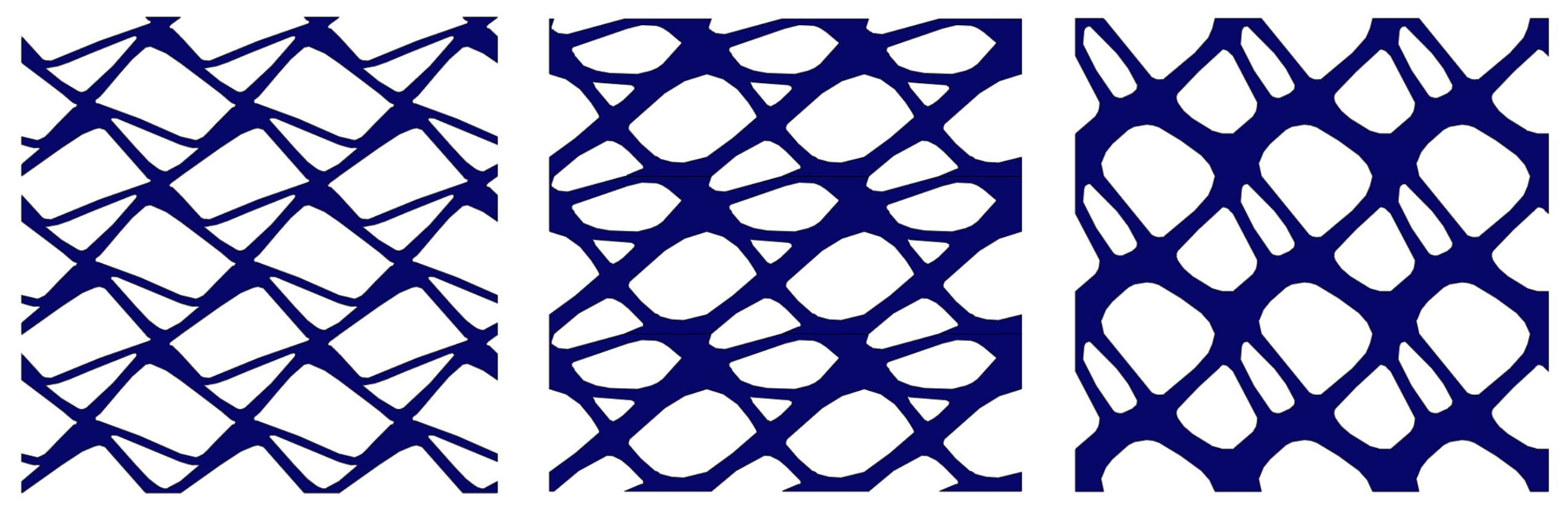
The MultiP-microSIMPATY algorithm provides original design solutions, complying also with conflicting requirements;
(ii)
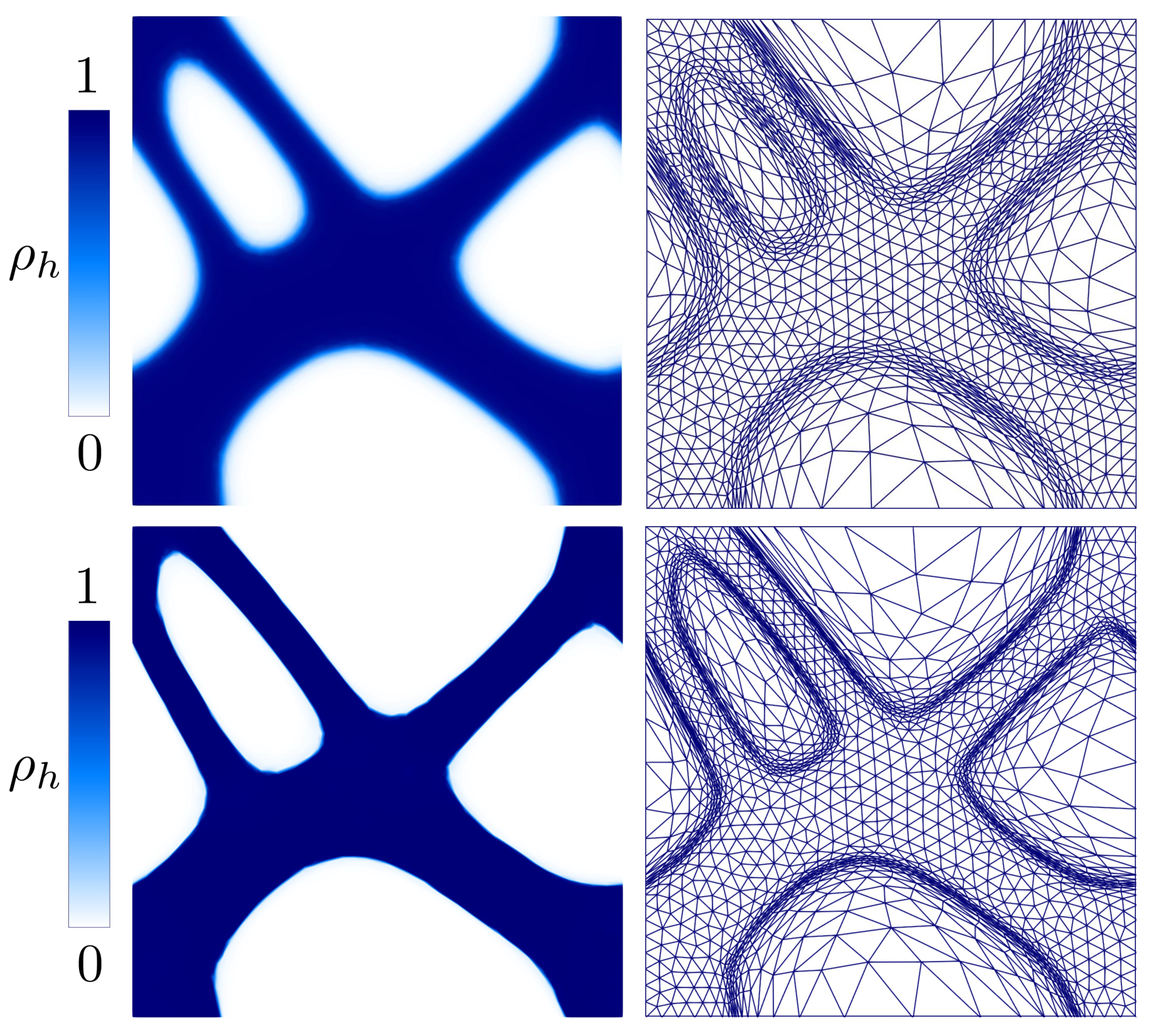
The good performance of microSIMPATY has been confirmed also in a thermo-elastic context. Standard issues typical of topology optimization, such as the presence of intermediate densities, of jagged boundaries, and of too complex structures, is mitigated by the employment of a mesh customized to the design process (see Figure 7 and Table 3);
(iii)
The new cellular materials have been successfully compared with consolidated solutions in terms of mechanical and thermal properties (see Table 2);
(iv)
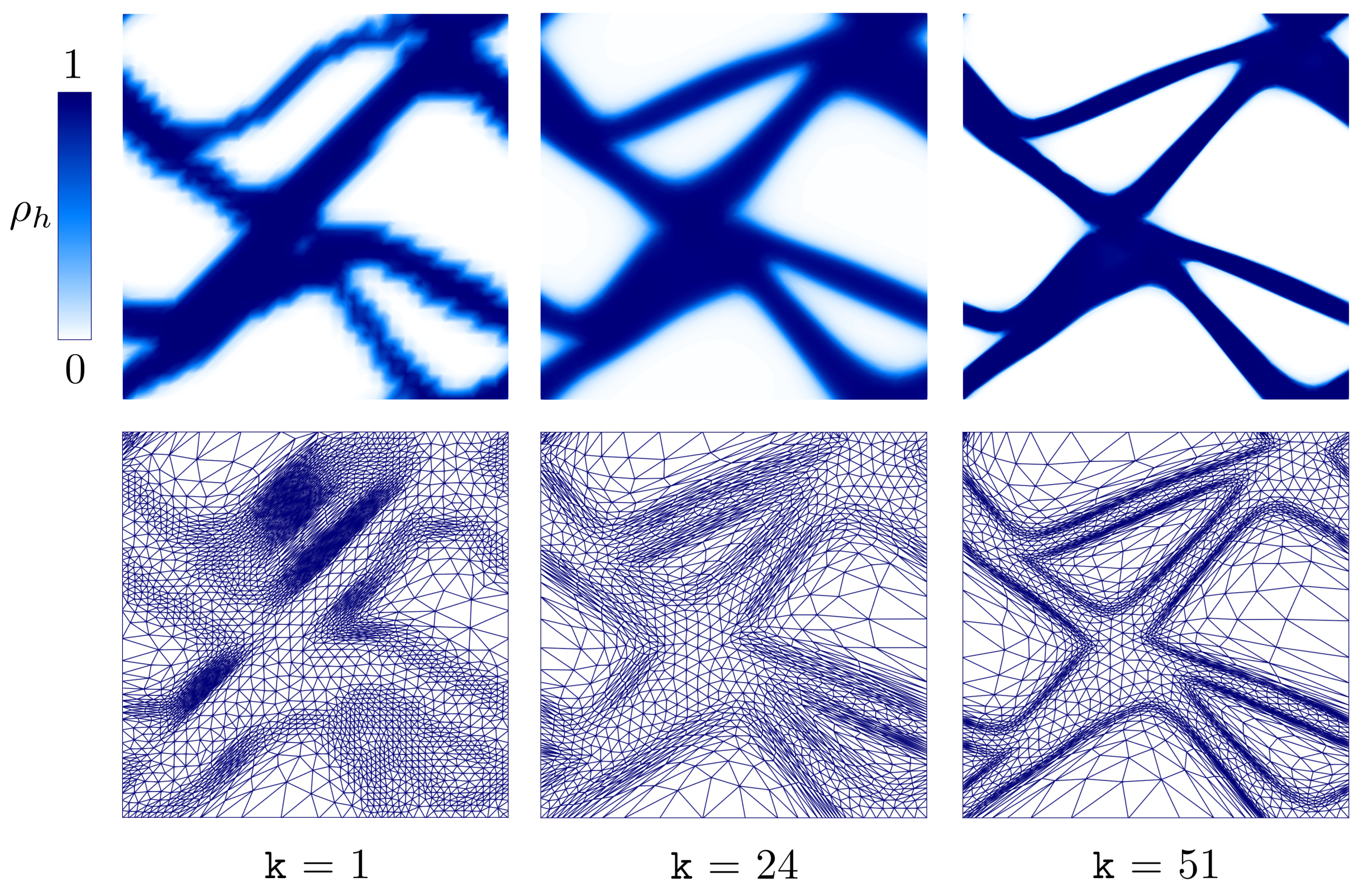
Filtering can be considerably limited thanks to the use of mesh adaptation. This turns into an improvement in terms of accuracy of the optimization process (see Figure 8);
(v)
The employment of an anisotropic mesh adaptation provides advantages with a view to a manufacturing phase. Indeed, the unit cells designed by MultiP-microSIMPATY exhibit very smooth geometries which demand for a very limited post-processing;
(vi)
The procedure here settled turns out to be fully general with respect to the selected multi-physics context.
Possible future developments include the extension of the MultiP-microSIMPATY design procedure to a 3D setting. The proposed methodology could also be exploited in a multiscale topology optimization framework [38], inspired by the many possible applications in engineering practice (including medicine, aerospace, automotive, and architecture). In such a context, with a view to the manufacturing step, another issue that deserves further investigation is represented by the handling of the transition area between different cellular materials. Finally, innovative techniques, such as model reduction or machine learning, still represent topics of high relevance in topology optimization for a future examination [63,64,65].

Author Contributions

Conceptualization, M.G., N.F., S.P. and S.F.; methodology, M.G., N.F. and S.P.; software, M.G. and N.F.; formal analysis, N.F. and S.P.; investigation, M.G., N.F., S.P. and S.F.; resources, S.P. and S.F.; data curation, M.G. and N.F.; writing—original draft preparation, M.G.; writing—review and editing, N.F. and S.P.; visualization, M.G. and N.F.; supervision, S.P. and S.F.; project administration, S.P. and S.F.; funding acquisition, S.P. and S.F. All authors have read and agreed to the published version of the manuscript.

Funding

This research received no external funding.

Acknowledgments

This research is part of the activity of the METAMatLab at Politecnico di Milano. The first and the last authors acknowledge the Italian Ministry of Education, University and Research for the support provided through the “Department of Excellence LIS4.0-Lightweight and Smart Structures for Industry 4.0” Project. The second author thanks the Istituto Nazionale di Alta Matematica (INdAM) for the awarded grant. Finally, the third author acknowledges the research project GNCS-INdAM 2020 “Tecniche Numeriche Avanzate per Applicazioni Industriali”.

Conflicts of Interest

The authors declare no conflict of interest.

References

  1. Gibson, L.J.; Ashby, M.F. Cellular Solids: Structure and Properties, 2nd ed.; Cambridge Solid State Science Series; Cambridge University Press: Cambridge, UK, 1997. [Google Scholar]
  2. Rashed, M.G.; Ashraf, M.; Mines, R.A.; Hazell, P.J. Metallic microlattice materials: A current state of the art on manufacturing, mechanical properties and applications. Mater. Des. 2016, 95, 518–533. [Google Scholar] [CrossRef]
  3. Bauer, J.; Hengsbach, S.; Tesari, I.; Schwaiger, R.; Kraft, O. High-strength cellular ceramic composites with 3D microarchitecture. Proc. Natl. Acad. Sci. USA 2014, 111, 2453–2458. [Google Scholar] [CrossRef] [PubMed] [Green Version]
  4. Schaedler, T.A.; Carter, W.B. Architected Cellular Materials. Annu. Rev. Mater. Res. 2016, 46, 187–210. [Google Scholar] [CrossRef]
  5. Ahmadi, S.M.; Campoli, G.; Amin Yavari, S.; Sajadi, B.; Wauthle, R.; Schrooten, J.; Weinans, H.; Zadpoor, A.A. Mechanical behavior of regular open-cell porous biomaterials made of diamond lattice unit cells. J. Mech. Behav. Biomed. Mater. 2014, 34, 106–115. [Google Scholar] [CrossRef] [PubMed]
  6. Yan, C.; Hao, L.; Hussein, A.; Young, P. Ti-6Al-4V triply periodic minimal surface structures for bone implants fabricated via selective laser melting. J. Mech. Behav. Biomed. Mater. 2015, 51, 61–73. [Google Scholar] [CrossRef] [Green Version]
  7. Taniguchi, N.; Fujibayashi, S.; Takemoto, M.; Sasaki, K.; Otsuki, B.; Nakamura, T.; Matsushita, T.; Kokubo, T.; Matsuda, S. Effect of pore size on bone ingrowth into porous titanium implants fabricated by additive manufacturing: An in vivo experiment. Mater. Sci. Eng. C 2016, 59, 690–701. [Google Scholar] [CrossRef] [Green Version]
  8. Arabnejad, S.; Burnett Johnston, R.; Pura, J.A.; Singh, B.; Tanzer, M.; Pasini, D. High-strength porous biomaterials for bone replacement: A strategy to assess the interplay between cell morphology, mechanical properties, bone ingrowth and manufacturing constraints. Acta Biomater. 2016, 30, 345–356. [Google Scholar] [CrossRef] [Green Version]
  9. Bandaru, P.R.; Vemuri, K.P.; Canbazoglu, F.M.; Kapadia, R.S. Layered thermal metamaterials for the directing and harvesting of conductive heat. AIP Adv. 2015, 5, 053403. [Google Scholar] [CrossRef] [Green Version]
  10. Liu, D.P.; Chen, P.J.; Huang, H.H. Realization of a thermal cloak-concentrator using a metamaterial transformer. Sci. Rep. 2018, 8, 1–11. [Google Scholar] [CrossRef] [Green Version]
  11. Attarzadeh, R.; Rovira, M.; Duwig, C. Design analysis of the “Schwartz D” based heat exchanger: A numerical study. Int. J. Heat Mass Transf. 2021, 177, 121415. [Google Scholar] [CrossRef]
  12. Kaur, I.; Singh, P. State-of-the-art in heat exchanger additive manufacturing. Int. J. Heat Mass Transf. 2021, 178, 121600. [Google Scholar] [CrossRef]
  13. Bendsøe, M.P.; Sigmund, O. Topology Optimization; Springer: Berlin/Heidelberg, Germany, 2004. [Google Scholar]
  14. Sigmund, O. Materials with prescribed constitutive parameters: An inverse homogenization problem. Int. J. Solids Struct. 1994, 31, 2313–2329. [Google Scholar] [CrossRef]
  15. Andreassen, E.; Andreasen, C.S. How to determine composite material properties using numerical homogenization. Comp. Mater. Sci. 2014, 83, 488–495. [Google Scholar] [CrossRef] [Green Version]
  16. Allaire, G.; Geoffroy-Donders, P.; Pantz, O. Topology optimization of modulated and oriented periodic microstructures by the homogenization method. Comput. Math. Appl. 2019, 78, 2197–2229. [Google Scholar] [CrossRef] [Green Version]
  17. Vigliotti, A.; Pasini, D. Mechanical properties of hierarchical lattices. Mech. Mat. 2013, 62, 32–43. [Google Scholar] [CrossRef] [Green Version]
  18. Wang, Y.; Xu, H.; Pasini, D. Multiscale isogeometric topology optimization for lattice materials. Comput. Methods. Appl. Mech. Eng. 2017, 316, 568–585. [Google Scholar] [CrossRef] [Green Version]
  19. Cheng, L.; Liu, J.; Liang, X.; To, A.C. Coupling lattice structure topology optimization with design-dependent feature evolution for additive manufactured heat conduction design. Comput. Methods Appl. Mech. Eng. 2018, 332, 408–439. [Google Scholar] [CrossRef]
  20. Panesar, A.; Abdi, M.; Hickman, D.; Ashcroft, I. Strategies for functionally graded lattice structures derived using topology optimisation for Additive Manufacturing. Addit. Manuf. 2018, 19, 81–94. [Google Scholar] [CrossRef]
  21. Moussa, A.; Rahman, S.; Xu, M.; Tanzer, M.; Pasini, D. Topology optimization of 3D-printed structurally porous cage for acetabular reinforcement in total hip arthroplasty. J. Mech. Behav. Biomed. Mater. 2020, 105, 103705. [Google Scholar] [CrossRef]
  22. Coelho, P.G.; Fernandes, P.R.; Guedes, J.M.; Rodrigues, H.C. A hierarchical model for concurrent material and topology optimisation of three-dimensional structures. Struct. Multidiscip. Optim. 2008, 35, 107–115. [Google Scholar] [CrossRef]
  23. Nakshatrala, P.B.; Tortorelli, D.A.; Nakshatrala, K.B. Nonlinear structural design using multiscale topology optimization. Part I: Static formulation. Comput. Methods Appl. Mech. Eng. 2013, 261/262, 167–176. [Google Scholar] [CrossRef]
  24. Djourachkovitch, T.; Blal, N.; Hamila, N.; Gravouil, A. Multiscale topology optimization of 3D structures: A micro-architectured materials database assisted strategy. Comput. Struct. 2021, 255, 106574. [Google Scholar] [CrossRef]
  25. Ferrer, A.; Oliver, J.; Cante, J.C.; Lloberas-Valls, O. Vademecum-based approach to multi-scale topological material design. Adv. Model. Simul. Eng. Sci. 2016, 3, 23. [Google Scholar] [CrossRef] [PubMed] [Green Version]
  26. Ferro, N.; Micheletti, S.; Perotto, S. Density-Based Inverse Homogenization with Anisotropically Adapted Elements. Lect. Notes Comput. Sci. Eng. 2020, 132, 211–221. [Google Scholar]
  27. di Cristofaro, D.; Galimberti, C.; Bianchi, D.; Ferrante, R.; Ferro, N.; Mannisi, M.; Perotto, S. Adaptive topology optimization for innovative 3D printed metamaterials. In Proceedings of the WCCM—ECCOMAS 2020 Conference, Volume 1200-Modeling and Analysis of Real World and Industry Applications, Online, 11–15 January 2021. [Google Scholar]
  28. Auricchio, F.; Bonetti, E.; Carraturo, M.; Hömberg, D.; Reali, A.; Rocca, E. A phase-field-based graded-material topology optimization with stress constraint. Math. Model. Methods Appl. Sci. 2020, 30, 1461–1483. [Google Scholar] [CrossRef]
  29. Huang, X.; Radman, A.; Xie, Y.M. Topological design of microstructures of cellular materials for maximum bulk or shear modulus. Comput. Mater. Sci. 2011, 50, 1861–1870. [Google Scholar] [CrossRef]
  30. Xia, L.; Breitkopf, P. Concurrent topology optimization design of material and structure within FE2 nonlinear multiscale analysis framework. Comput. Methods Appl. Mech. Eng. 2014, 278, 524–542. [Google Scholar] [CrossRef]
  31. Wang, Y.; Luo, Z.; Zhang, N.; Kang, Z. Topological shape optimization of microstructural metamaterials using a level set method. Comput. Mater. Sci. 2014, 87, 178–186. [Google Scholar] [CrossRef]
  32. Torquato, S.; Hyun, S.; Donev, A. Optimal design of manufacturable three-dimensional composites with multifunctional characteristics. J. Appl. Phys. 2003, 94, 5748–5755. [Google Scholar] [CrossRef] [Green Version]
  33. de Kruijf, N.; Zhou, S.; Li, Q.; Mai, Y.W. Topological design of structures and composite materials with multiobjectives. Int. J. Solids Struct. 2007, 44, 7092–7109. [Google Scholar] [CrossRef]
  34. Challis, V.J.; Roberts, A.P.; Wilkins, A.H. Design of three dimensional isotropic microstructures for maximized stiffness and conductivity. Int. J. Solids Struct. 2008, 45, 4130–4146. [Google Scholar] [CrossRef] [Green Version]
  35. Vineyard, E.; Gao, X.L. Topology and shape optimization of 2-d and 3-d micro-architectured thermoelastic metamaterials using a parametric level setmethod. CMES-Comput. Model. Eng. Sci. 2021, 127, 819–854. [Google Scholar]
  36. Sigmund, O.; Petersson, J. Numerical instabilities in topology optimization: A survey on procedures dealing with checkerboards, mesh-dependencies and local minima. Struct. Optim. 1998, 16, 68–75. [Google Scholar] [CrossRef]
  37. Micheletti, S.; Perotto, S.; Soli, L. Topology optimization driven by anisotropic mesh adaptation: Towards a free-form design. Comput. Struct. 2019, 214, 60–72. [Google Scholar] [CrossRef]
  38. Ferro, N.; Perotto, S.; Bianchi, D.; Ferrante, R.; Mannisi, M. Design of cellular materials for multiscale topology optimization: Application to patient-specific orthopedic devices. Struct. Multidiscip. Optim. 2021, 28, 2021. [Google Scholar] [CrossRef]
  39. Hassani, B.; Hinton, E. A review of homogenization and topology optimization I—homogenization theory for media with periodic structure. Comput. Struct. 1998, 69, 707–717. [Google Scholar] [CrossRef]
  40. Hassani, B.; Hinton, E. A review of homogenization and topology opimization II—analytical and numerical solution of homogenization equations. Comput. Struct. 1998, 69, 719–738. [Google Scholar] [CrossRef]
  41. Terada, K.; Hori, M.; Kyoya, T.; Kikuchi, N. Simulation of the multi-scale convergence in computational homogenization approaches. Int. J. Solids Struct. 2000, 37, 2285–2311. [Google Scholar] [CrossRef]
  42. Gould, P.L. Introduction to Linear Elasticity; Springer: New York, NY, USA, 1994. [Google Scholar]
  43. Noël, L.; Duysinx, P. Shape optimization of microstructural designs subject to local stress constraints within an XFEM-level set framework. Struct. Multidiscip. Optim. 2017, 55, 2323–2338. [Google Scholar] [CrossRef]
  44. Ern, A.; Guermond, J.L. Theory and Practice of Finite Elements; Springer: New York, NY, USA, 2004. [Google Scholar]
  45. Formaggia, L.; Perotto, S. New anisotropic a priori error estimates. Numer. Math. 2001, 89, 641–667. [Google Scholar] [CrossRef]
  46. Ainsworth, M.; Oden, J.T. A Posteriori Error Estimation in Finite Element Analysis; John Wiley & Son: New York, NY, USA, 2000. [Google Scholar]
  47. Bangerth, W.; Rannacher, R. Adaptive Finite Element Methods for Differential Equations; Birkhäuser Verlag: Basel, Germany, 2003. [Google Scholar]
  48. Zienkiewicz, O.C.; Zhu, J.Z. A simple error estimator and adaptive procedure for practical engineerng analysis. Int. J. Numer. Methods Eng. 1987, 24, 337–357. [Google Scholar] [CrossRef]
  49. Zienkiewicz, O.C.; Zhu, J.Z. The superconvergent patch recovery and a posteriori error estimates. I: The recovery technique. Int. J. Numer. Meth. Eng. 1992, 33, 1331–1364. [Google Scholar] [CrossRef]
  50. Rodríguez, R. Some remarks on Zienkiewicz-Zhu estimator. Numer. Methods Partial. Differ. Equations 1994, 10, 625–635. [Google Scholar] [CrossRef]
  51. Maisano, G.; Micheletti, S.; Perotto, S.; Bottasso, C.L. On some new recovery-based a posteriori error estimators. Comput. Methods Appl. Mech. Eng. 2006, 195, 4794–4815. [Google Scholar] [CrossRef]
  52. Li, X.D.; Wiberg, N.E. A posteriori error estimate by element patch post-processing, adaptive analysis in energy and L2 norms. Comput. Struct. 1994, 53, 907–919. [Google Scholar] [CrossRef]
  53. Micheletti, S.; Perotto, S. Anisotropic adaptation via a Zienkiewicz-Zhu error estimator for 2D elliptic problems. In Numerical Mathematics and Advanced Applications; Kreiss, G., Lötstedt, P., Målqvist, A., Neytcheva, M., Eds.; Springer: Berlin/Heidelberg, Germany, 2010; pp. 645–653. [Google Scholar]
  54. Farrell, P.E.; Micheletti, S.; Perotto, S. An anisotropic Zienkiewicz-Zhu-type error estimator for 3D applications. Int. J. Numer. Meth. Eng. 2011, 85, 671–692. [Google Scholar] [CrossRef]
  55. Micheletti, S.; Perotto, S. Reliability and efficiency of an anisotropic Zienkiewicz-Zhu error estimator. Comput. Methods Appl. Mech. Eng. 2006, 195, 799–835. [Google Scholar] [CrossRef]
  56. Ferro, N.; Micheletti, S.; Perotto, S. Compliance-stress constrained mass minimization for topology optimization on anisotropic meshes. SN Appl. Sci. 2020, 2, 1–11. [Google Scholar] [CrossRef]
  57. Ferro, N.; Micheletti, S.; Perotto, S. An optimization algorithm for automatic structural design. Comput. Methods Appl. Mech. Eng. 2020, 372, 113335. [Google Scholar] [CrossRef]
  58. Hecht, F. New development in FreeFem++. J. Numer. Math. 2012, 20, 251–265. [Google Scholar] [CrossRef]
  59. Wächter, A.; Lorenz, T. Biegler. On the implementation of an interior-point filter line-search algorithm for large-scale nonlinear programming. Math. Program. 2006, 106, 25–57. [Google Scholar] [CrossRef]
  60. Svanberg, K. The method of moving asymptotes-a new method for structural optimization. Int. J. Numer. Meth. Eng. 1987, 24, 359–373. [Google Scholar] [CrossRef]
  61. Lazarov, B.S.; Sigmund, O. Filters in topology optimization based on Helmholtz-type differential equations. Int. J. Numer. Meth. Eng. 2011, 86, 765–781. [Google Scholar] [CrossRef]
  62. Sigmund, O. Morphology-based black and white filters for topology optimization. Struct. Multidiscip. Optim. 2007, 33, 401–424. [Google Scholar] [CrossRef] [Green Version]
  63. Caicedo, M.; Mroginski, J.L.; Toro, S.; Raschi, M.; Huespe, A.; Oliver, J. High performance reduced order modeling techniques based on optimal energy quadrature: Application to geometrically non-linear multiscale inelastic material modeling. Arch. Comput. Methods Eng. 2019, 26, 771–792. [Google Scholar] [CrossRef]
  64. Ferro, N.; Micheletti, S.; Perotto, S. POD-assisted strategies for structural topology optimization. Comput. Math. Appl. 2019, 77, 2804–2820. [Google Scholar] [CrossRef]
  65. Chi, H.; Zhang, Y.; Tang, T.L.E.; Mirabella, L.; Dalloro, L.; Song, L.; Paulino, G.H. Universal machine learning for topology optimization. Comput. Methods. Appl. Mech. Eng. 2021, 375, 112739. [Google Scholar] [CrossRef]
Figure 1. Initial guess ρ h 0 (left) and corresponding mesh T h 0 (right).
Mca 27 00015 g001
Figure 2. Design Case 1: density field (top) and associated anisotropic adapted mesh (bottom) for three different global iterations.
Mca 27 00015 g002
Figure 3. Design Case 1: evolution of the objective functional M and of the constraints c i (top); trend of the mesh cardinality # T h (bottom) throughout the global iterations k.
Mca 27 00015 g003
Figure 4. Design Cases 1, 2, and 3 (leftright): 3 × 3 -cell meta-material.
Mca 27 00015 g004
Figure 5. Design Case 2: density field (top) and associated anisotropic adapted mesh (bottom) for three different global iterations.
Mca 27 00015 g005
Figure 6. Design Case 3: density field (top) and associated anisotropic adapted mesh (bottom) for three different global iterations.
Mca 27 00015 g006
Figure 7. Comparison between the optimized cells delivered by MultiP.microSIMP (top) and by MultiP-microSIMPATY (bottom) for the Design Cases 1, 2, and 3 (from left to right).
Mca 27 00015 g007
Figure 8. Effect of filtering for the MultiP-microSIMPATY algorithm: density field (left) and associated anisotropic adapted mesh (right) when filtering is applied during the whole optimization process (top) and in the first 25 iterations only (bottom).
Mca 27 00015 g008
Table 1. Design cases 1, 2, and 3: values of the constraints and of the objective functional computed with Abaqus software, together with the lower and the upper bounds, c l and c u , involved in the optimization.
E 1111 H E 1212 H E 2222 H E 1111 H k 11 H k 22 H k 11 H M
Design Case 1
c u 0.0800.0802.0001.0000.580
c0.0380.0561.2990.1990.566
c l 0.0500.0551.0000.0100.0000.292
Design Case 2
c u 0.3500.1502.0001.0002.000
c0.2500.0860.2990.3170.597
c l 0.2300.0800.3000.3000.0000.412
Design Case 3
c u 0.1500.1001.1000.4001.100
c0.1510.0831.0740.2601.002
c l 0.1000.0801.0000.2501.0000.415
Table 2. Comparison between the MultiP-microSIMPATY optimized structures and off-the-shelf designs in terms of homogenized elastic and thermal properties, for comparable volume fraction values.
E x H E y H G H k 11 H k 22 H
Design Case 1
D1 Mca 27 00015 i0010.0120.0150.0560.2000.113
A Mca 27 00015 i0020.0090.0090.0750.1630.163
B Mca 27 00015 i0030.0950.0420.0590.1980.131
Design Case 2
D2 Mca 27 00015 i0040.1260.0390.0820.3170.126
C Mca 27 00015 i0050.3410.1160.0020.4320.125
Design Case 3
D3 Mca 27 00015 i0060.0700.0700.0820.2600.261
L Mca 27 00015 i0070.1880.1880.0720.2550.255
Table 3. Comparison between the optimized cells delivered by MultiP-microSIMPATY and a standard inverse homogenization algorithm in terms of mass.
D1D2D3
MultiP-microSIMP0.3300.4430.486
MultiP-microSIMPATY0.2920.4120.415
Mass reduction [%]11.5%7.0%14.6%
Publisher’s Note: MDPI stays neutral with regard to jurisdictional claims in published maps and institutional affiliations.

