Mathematical Modeling and Characterization of the Spread of Chikungunya in Colombia

Abstract

The Chikungunya virus is the cause of an emerging disease in Asia and Africa, and also in America, where the virus was first detected in 2006. In this paper, we present a mathematical model of the Chikungunya epidemic at the population level that incorporates the transmission vector. The epidemic threshold parameter ${\mathcal{R}}_0$ for the extinction of disease is computed using the method of the next generation matrix, which allows for insights about what are the most relevant model parameters. Using Lyapunov function theory, some sufficient conditions for global stability of the the disease-free equilibrium are obtained. The proposed mathematical model of the Chikungunya epidemic is used to investigate and understand the importance of some specific model parameters and to give some explanation and understanding about the real infected cases with Chikungunya virus in Colombia for data belonging to the year 2015. In this study, we were able to estimate the value of the basic reproduction number ${\mathcal{R}}_0$. We use bootstrapping and Markov chain Monte Carlo techniques in order to study parameters’ identifiability. Finally, important policies and insights are provided that could help government health institutions in reducing the number of cases of Chikungunya in Colombia.

1. Introduction

The Chikungunya virus is a type of arbovirus, so it is only transmitted by hematopoietic arthropods that become infected after biting some vertebrates. Later, the arthropods can transmit the virus to a susceptible vertebrate through a bite [1]. The arthropod vectors are usually Aedes aegypti and Ae. albopictus [2,3,4]. The virus has had mutations, allowing Aedes albopictus to transmit the disease [5]. The Chikungunya disease originated in Sub-Saharan Africa, and it has become endemic in Africa, where there is a natural transmission between mosquitoes and primates to humans [3]. The Chikungunya disease is an emerging disease in Asia. In America, it was detected in 2006, and there is an imminent risk of the virus spreading throughout South America. In the last few years, several outbreaks have occurred on the island of Reunion, in Cambodia, Comoros, Mayotte, Madagascar, Mauritius, Italy, Seychelles, and the Maldives [3,6,7,8]. The first outbreak in Europe was in the warm northeast region of Italy in July 2007. Probably, the virus came from Kerala (India), where the disease was at its highest peak [7]. The Chikungunya disease causes arthritis, fever, and pain of the joints. Symptoms of chikungunya are generally resolved within 7–10 days, but some patients are plagued with chronic arthralgia, which could persist for months or years [9,10,11]. There is no vaccine for the Chikungunya virus at this moment that could be used to restrict and control the transmission of the disease [6,12]. Moreover, no effective drug is available for human use for any alphavirus, although analgesics and non-steroidal anti-inflammatory drugs can provide relief from symptoms [12]. The incubation of the virus lasts between 5–12 days and the infectious stage between 5–15 days, in both primates and humans [13,14].

As mentioned above, the Chikungunya virus is spreading around the world, and due to world climate change, it is expected that more regions are going to be reached by it. For instance, in [15], the authors presented results regarding the risk of Zika and Chikungunya virus transmission in human population centers of the eastern United States. In this way, in order to better understand the dynamics of how the Chikungunya virus is transmitted, we propose and analyze a mathematical model given by a system of nonlinear differential equations where the populations of hosts and mosquitoes are homogeneous. This mathematical modeling approach is the standard way to study the dynamical behavior of diseases in populations from an epidemiological point of view [16,17,18,19]. In particular, there is a variety of models for vector-borne diseases. For instance, in [20], the authors proposed a mathematical model for vector-borne disease with delay to consider the incubation period. In addition, in [21], the authors used optimal control to minimize the number of infections. Recently, some works extended these types of models using versatile fractional derivatives [22,23,24].

In [25], the authors proposed a deterministic mathematical model for Chikungunya infection considering that there is transmission of the virus between humans and mosquitoes. The authors used two infected human subpopulations designated as symptomatic and asymptomatic to classify the humans responsible for transmitting the virus. Additionally, they considered the subpopulation of humans carrying the virus, but had no possibility of spreading it. In this paper, the authors demonstrated the influence of humans on the infection of the latency period. They also remarked about the necessity of fitting the model to real data so that it will be useful in controlling the spread of the virus. Another interesting work was presented in [26], where the authors proposed a mathematical model of three age-structured transmissions of Chikungunya virus. The authors divided the human population into juvenile, adult, and senior subpopulations.

In [6], the authors proposed a stochastic mathematical model for a rural region in Cambodia, considering the fact that a stochastic model fits data better in small populations. These authors also used a subgroup of latent human and mosquito individuals and additionally included a larvae subgroup in the mosquito population. An innovation in that work is the introduction of three subclasses of infected humans. Other mathematical models for the Chikungunya virus propagation that include the latency stage were given in [27,28,29].

In the present work, our aim is to understand and explain some dynamics regarding the prevalence of Chikungunya infection in Colombia. The mathematical model is important since in practice, there are few economic resources to tackle or fight the Chikungunya virus’ spread. Thus, the model allows one to decide on the best or most convenient health policies. In the proposed model, we consider a chronic subpopulation that has not been considered previously. The people in this particular class cannot transmit the disease, but have some types of chronic rheumatic symptoms. The main reason to consider this class is that health institutions are interested in the number of chronic cases of Chikungunya and its evolution. In addition, the latency stage for the human and mosquito populations is also introduced in the mathematical model, since this stage is observed in the real world. Although the virus may also spread to other vertebrate populations such as primates [30,31,32,33], reservoirs different from humans are not included in the analysis, since in Colombia, known cases are all human. However, future work might include reservoirs different from humans and would increase the complexity of the mathematical model and of the fitting process to the real data.

Numerical simulations are performed to support the theoretical results. In addition, the proposed mathematical model of Chikungunya is used to explain and understand the infected cases with the Chikungunya virus in Colombia. In particular, we use the proposed Chikungunya mathematical model to perform a fitting process to real data of Colombia. Additionally, we used bootstrapping and Markov chain Monte Carlo techniques in order to do analysis of the parameters’ identifiability [34,35,36,37,38,39,40]. Finally, important policies and insights are provided that could help government health institutions in lowering the infected cases with the Chikungunya virus in Colombia.

The paper is organized as follows. In Section 2, the mathematical model of Chikungunya is presented together with a set of definitions and basic underlying hypotheses. The proposed Chikungunya mathematical model is analyzed in Section 3. The fitting process and numerical simulations are presented in Section 4. Next, the parameter estimation of the model for a Colombia case using Markov chain Monte Carlo, as well as bootstrapping is performed in Section 5. The last part, Section 6, is devoted to the discussion and conclusions.

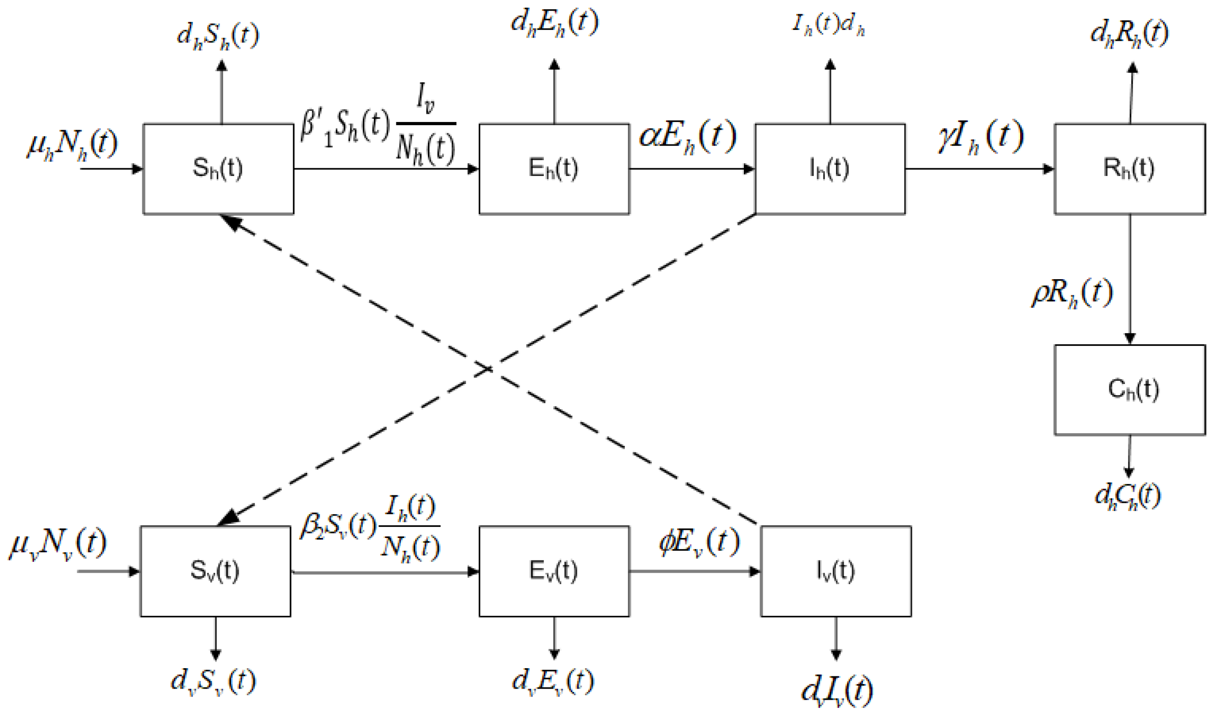
2. Mathematical Model

In this section, we set out a continuous mathematical model for the transmission and evolution of the Chikungunya infection in the human and mosquito populations. In the proposed mathematical model, vertical transmission is not included because the number of cases is small when compared to the total number of infected cases. However, if the virus prevalence increases in the female population, it may be necessary to include it in the proposed model. Furthermore, we do not consider a vaccinated class since there are no vaccines on the market [12,41].

The proposed model of the Chikungunya virus transmission dynamics incorporates a cross-transmission between the human and vector populations. In particular, it is assumed that the Chikungunya virus spreads by the effective contact between a mosquito infected with a human susceptible, and vice versa. This contact depends on different environmental factors. Some factors to consider are: the weather, the temperature, the altitude, and the mosquito bite rate. Varying these values will generate different degrees of the probability of the transmission of the disease. Here, we will not include seasonal effects or variability in the populations. Using a population-based approach of an epidemiological type, the population of humans is divided into five groups: susceptibles, latents, infected, recovered, and the ones with chronic rheumatic symptoms. It is important to remark that the people with chronic rheumatic symptoms do not have the Chikungunya virus, just some symptoms related to it, since they were infected previously. In addition, the population of the vector is divided into three groups: susceptible vector, latent vector, and infected vector. The resulting mathematical model is a nonlinear system of eight ordinary differential equations, which is analyzed to find the equilibrium points and their stability, including the well-known epidemic threshold parameter known as the basic reproduction number, $R_0$. We estimate some of the unknown key epidemiological parameters of the model from real data, which allow us to compute $R_0$, defined as the average number of secondary cases generated by a typical infectious individual in a fully-susceptible population. Moreover, we are able to compute approximately how many individuals are infected during an outbreak. All these estimates can help assist with outbreak planning, assessment of health strategies, and the design of future research regarding Chikungunya infection transmission.

Thus, following the basic ideas and structure of mathematical modeling in epidemiology, the Chikungunya model will be developed under the following basic hypotheses [16,17]:

• The total population of humans $N_h(t)$ is divided into five subpopulations: humans who may become infected (susceptible $S_h(t)$), humans exposed, but still not infected due to the existence of an incubation period of the virus (latent $E_h(t)$), humans infected by the Chikungunya virus and that develop the disease (infected $I_h(t)$), humans who have recovered from the Chikungunya infection (recovered $R_h(t)$), and humans who have the disease chronically (chronic $C_h(t)$).
• The parameter ${\mu }_h$ is the birth rate of humans. The birth rate ${\mu }_h$ is assumed equal to natural death $d_h$.
• The mortality rate increase due to the disease is a real fact. However, since this rate is small in comparison with other rates and is not going to affect the dynamics, we assume that $ϵ=0$.
• The total population of mosquitoes $N_v(t)$ is divided into three subpopulations: mosquitoes who may become infected (susceptible $S_v(t)$), mosquitoes in a latent stage (latent $E_v(t)$), and mosquitoes currently infected or spreading the Chikungunya virus (infected $I_v(t)$).
• The parameter ${\mu }_v$ is the birth rate of the mosquitoes, and it is assumed equal to the death rate $d_v$.
• A susceptible human can transit to the latent subpopulation $E_h(t)$ because of an effective transmission due to a bite of an infected mosquito at a rate of ${\beta }_1^{\prime }$.
• A susceptible mosquito can be infected if there exists an effective transmission when it bites an infected human, at a rate ${\beta }_2$.
• A fraction $\alpha$ of the latent humans passes to infected by the virus.
• A fraction $\gamma$ of the infected humans recovers, i.e., they do not have the disease anymore.
• A fraction $\rho$ of the recovered humans moves to the chronic class.
• A fraction $\varphi$ of the latent mosquitoes goes through to infected mosquitoes.
• Homogeneous mixing is assumed, i.e., all susceptible humans have the same probability of being infected and all susceptible mosquitoes have the same probability of being infected.

It is important to notice that the parameter ${\beta }_1^{\prime }$ depends on two different parameter: the bite rate of an infected mosquito on susceptible people and the probability per bite to transmit the virus from the mosquito to the human. On the other hand, ${\beta }_2$ depends on the bite rate of a susceptible mosquito on an infected human and the probability per bite to transmit the virus from the human to the vector. In reality, these parameters are very difficult to estimate due to different environment conditions. Thus, the values of these parameters are most likely to vary from one region to another. In fact, the values might be very different for rural and urban areas. We assume that the natural birth rate is equal to the natural death rate for the human population since we are interested in fitting the model to the real data of the year 2015 and study the identifiability of the parameters. This is considered a short period where the births can be balanced with deaths. For instance, in [25], the authors did not even consider the births and deaths, even though these might affect the dynamics. For mosquitoes, there are no reliable data; thus, we adopted a conservative approach similar to the one used in [25]. The model could be expanded to consider the variation of mosquito populations. This can be done adding a seasonal forcing function [42], but will introduce additional parameters to the model. Furthermore, it will compromise the identifiability more, which currently is an important issue.

Under the above hypotheses, the following diagram illustrates the interactions of the Chikungunya infection in human and mosquito populations; see Figure 1.

The corresponding mathematical model is given by the following system of ordinary differential equations:

$$\begin{array}{ccc}\hfill {\dot{S}}_h(t)& =& {\mu }_h{N}_h(t)-S_h(t)({\beta }_1^{\prime }{\displaystyle \frac{I_v(t)}{N_h(t)}}+d_h),\hfill \\ \hfill {\dot{E}}_h(t)& =& {\beta }_1^{\prime }{S}_h(t){\displaystyle \frac{I_v(t)}{N_h(t)}}-E_h(t)(d_h+\alpha ),\hfill \\ \hfill {\dot{I}}_h(t)& =& \alpha E_h(t)-I_h(t)[d_h+\gamma ],\hfill \\ \hfill {\dot{R}}_h(t)& =& \gamma I_h(t)-R_h(t)(\rho +d_h),\hfill \\ \hfill {\dot{C}}_h(t)& =& \rho R_h(t)-d_h{C}_h(t),\hfill \\ \hfill {\dot{S}}_v(t)& =& {\mu }_v{N}_v(t)-S_v(t)({\beta }_2{\displaystyle \frac{I_h(t)}{N_h(t)}}+d_v),\hfill \\ \hfill {\dot{E}}_v(t)& =& {\beta }_2{S}_v(t){\displaystyle \frac{I_h(t)}{N_h(t)}}-E_v(t)(d_v+\varphi ),\hfill \\ \hfill {\dot{I}}_v(t)& =& \varphi E_v(t)-d_v{I}_v(t).\hfill \end{array}$$

(1)

Adding the first five equations, one gets:

$${\dot{N}}_h(t)={\dot{S}}_h(t)+{\dot{E}}_h(t)+{\dot{I}}_h(t)+{\dot{R}}_h(t)+{\dot{C}}_h(t)=0$$

and therefore, the human population is constant. Analogously, by adding the last three equations, we have that:

$${\dot{N}}_v(t)={\dot{S}}_v(t)+{\dot{E}}_v(t)+{\dot{I}}_v(t)=0$$

and likewise, the mosquito populations is constant. Thus, we will denote $N_h(t)=N_h$ and $N_v(t)=N_v$, without dependency on time.

All parameters in this model are non-negative. It is easy to prove that the system (1) is well-posed, in the sense that if the initial data $({\dot{S}}_h(0),{\dot{E}}_h(0),{\dot{I}}_h(0),$ ${\dot{R}}_h(0),{\dot{C}}_h(0),{\dot{S}}_v(0),{\dot{E}}_v(0),{\dot{I}}_v(0))$ are in the region ${\mathbb{R}}_{+}^8$, then the solutions will be defined for all time $t\ge 0$ and remain in this region.

Normalizing the human and mosquito populations,

$$s_h(t)={\displaystyle \frac{S_h(t)}{N_h(t)}},e_h(t)={\displaystyle \frac{E_h(t)}{N_h(t)}},i_h(t)={\displaystyle \frac{I_h(t)}{N_h(t)}},r_h(t)={\displaystyle \frac{R_h(t)}{N_h(t)}},c_h(t)={\displaystyle \frac{C_h(t)}{N_h(t)}},$$

and:

$$s_v(t)={\displaystyle \frac{S_v(t)}{N_v(t)}},e_v(t)={\displaystyle \frac{E_v(t)}{N_v(t)}},i_v(t)={\displaystyle \frac{I_v(t)}{N_v(t)}}.$$

Using the assumptions ${\mu }_h=d_h$ and ${\mu }_v=d_v$, one can obtain the following system that describes the dynamics of Chikungunya in each class:

$$\begin{array}{ccc}\hfill {\dot{s}}_h(t)& =& d_h-s_h(t)({\beta }_1{i}_v(t)+d_h),\hfill \\ \hfill {\dot{e}}_h(t)& =& {\beta }_1{s}_h(t)i_v(t)-e_h(t)(d_h+\alpha ),\hfill \\ \hfill {\dot{i}}_h(t)& =& \alpha e_h(t)-i_h(t)[d_h+\gamma ],\hfill \\ \hfill {\dot{r}}_h(t)& =& \gamma i_h(t)-r_h(t)(\rho +d_h),\hfill \\ \hfill {\dot{c}}_h(t)& =& \rho r_h(t)-d_h{c}_h(t),\hfill \\ \hfill {\dot{s}}_v(t)& =& d_v-s_v(t)({\beta }_2{i}_h(t)+d_v),\hfill \\ \hfill {\dot{e}}_v(t)& =& {\beta }_2{s}_v(t)i_h(t)-e_v(t)(d_v+\varphi ),\hfill \\ \hfill {\dot{i}}_v(t)& =& \varphi e_v(t)-d_v{i}_v(t).\hfill \end{array}$$

(2)

where ${\beta }_1=m{\beta }_1^{\prime }=\frac{N_v}{N_h}{\beta }_1^{\prime }$. Now, we can define a more specific region, $\mathsf{\Omega }=\{(s_h(t),e_h(t),i_h(t),c_h(t),s_v(t),e_v(t),i_v(t))\in {[0,1]}^8\},$ and the solutions will be defined for all time $t\ge 0$ and remain in this region $\mathsf{\Omega }.$

3. Analysis of the Model

3.1. Equilibrium Points and Local Stability of the Chikungunya Mathematical Model

Setting the right-hand side of Equation (2) equal to zero, we can find the equilibrium points of the model. The first point is denoted as the disease-free equilibrium (DFE), and the other is called the endemic equilibrium (EE). Thus, we obtain the equilibrium point $DFE=(1,0,0,0,0,1,0,0)$. On the other hand, the mathematical expression of the other equilibrium point $EE=(S_h^{\ast },E_h^{\ast },I_h^{\ast },R_h^{\ast },C_h^{\ast },S_v^{\ast },E_v^{\ast },I_v^{\ast })$, is extremely long. Therefore, we will present this endemic equilibrium (EE) in terms of $I_h^{\ast }$. It is important to mention that our main interest is to obtain the conditions under which the population is free of disease. We will discuss later the endemic equilibria and under which conditions they exist.

For infectious diseases, the basic reproduction number is denoted as ${\mathcal{R}}_0$ and is one of the most useful threshold parameters. It can help determine whether or not an infectious disease will spread throughout a population [43,44]. ${\mathcal{R}}_0$ also has been used for social epidemics [18,45].

In order to compute the basic reproduction number ${\mathcal{R}}_0$ for the mathematical model (2), we apply the next generation technique as proposed in [43,44,46]. The infectious classes in this model are $e_h(t)$, $i_h(t)$, $e_v(t)$, and $i_v(t)$. Thus, at the $DFE$, one gets,

$$\mathit{F}=\left[\begin{array}{cccc}0& 0& 0& {\beta }_1\\ 0& 0& 0& 0\\ 0& {\beta }_2& 0& 0\\ 0& 0& 0& 0\end{array}\right],$$

and:

$$\mathit{V}=\left[\begin{array}{cccc}\alpha +d_h& 0& 0& 0\\ -\alpha & d_h+\gamma & 0& 0\\ 0& 0& d_v+\varphi & 0\\ 0& 0& -\varphi & d_v\end{array}\right],$$

$$\mathit{K}=\left[\begin{array}{cccc}0& 0& \frac{{\beta }_1\varphi }{d_v(d_v+\varphi )}& \frac{{\beta }_1}{d_v}\\ 0& 0& 0& 0\\ \frac{{\beta }_2(\alpha d_v^2+\alpha d_v\varphi )}{(\alpha +d_h)d_v(d_h+\gamma )(d_v+\varphi )}& \frac{{\beta }_2}{d_h+\gamma }& 0& 0\\ 0& 0& 0& 0\end{array}\right],$$

where the matrix F is related to the rate of increase of secondary infections and V to the rate of the disease progression, death, and recovery. The next generation matrix, $K=F{V}^{-1}$, is non-negative, and therefore, it has a non-negative eigenvalue ${\mathcal{R}}_0=\rho (F{V}^{-1})$ and a non-negative eigenvector $\omega$ associated with ${\mathcal{R}}_0$ [43,46].

There are no other eigenvalues of the matrix K with modulus greater than ${\mathcal{R}}_0$. Therefore, applying the next generation matrix, we obtain:

$${\mathcal{R}}_0=\sqrt{\frac{{\beta }_1{\beta }_2\alpha \varphi }{(\alpha +d_h)d_v(d_h+\gamma )(d_v+\varphi )}},$$

(3)

or in a more compact form:

$${\mathcal{R}}_0=\sqrt{{\displaystyle \frac{{\beta }_1{\beta }_2\alpha \varphi }{ABC{d}_v}}},$$

where $A=(\alpha +d_h),$ $B=(d_h+\gamma ),$ and $C=(d_v+\varphi ).$

Thus, we obtain the following theorem [43,44]:

Theorem 1.

The disease-free equilibrium $DFE$ is locally asymptotically stable for ${\mathcal{R}}_0<1$ and unstable for${\mathcal{R}}_0>1.$

This analysis shows that when the threshold parameter $R_0$ is less than unity, the disease disappears, while the opposite results show an endemic equilibrium in the human population.

Notice that the basic reproduction number ${\mathcal{R}}_0$ has in the numerator all the factors that contribute to having an epidemic outbreak. For instance, we have the Chikungunya transmissibility ${\beta }_1$ from an infected vector to a susceptible human and the Chikungunya transmissibility ${\beta }_2$ from an infected human to a susceptible vector. In addition, we have the incubation rates of the virus for humans and mosquitoes $\alpha$ and $\varphi$, respectively. Notice that both chronic and recovered classes have a limited role in the Chikungunya dynamics, since their equations are in some sense uncoupled from the rest of the model and do not play a role in the threshold parameter $R_0$.

3.2. Endemic Equilibria

In order to find the endemic equilibrium point, we set the right-hand side of Equation (2) equal to zero, and at least one of the infected components of the model (2) is different than zero. Let $EE=(S_h^{\ast },E_h^{\ast },I_h^{\ast },R_h^{\ast },C_h^{\ast },S_v^{\ast },E_v^{\ast },I_v^{\ast })$ represent any arbitrary endemic equilibrium point. Solving the equations for the steady state, we obtain:

$$S_h^{\ast }={\displaystyle \frac{ABC(d_v+{\beta }_2{I}_h^{\ast })}{\alpha \varphi {\mu }_v{\beta }_1{\beta }_2}},E_h^{\ast }={\displaystyle \frac{B}{\alpha }}{I}_h^{\ast },R_h^{\ast }={\displaystyle \frac{\gamma }{\rho +d_h}}{I}_h^{\ast },$$

$$C_h^{\ast }={\displaystyle \frac{\rho \gamma }{d_h(\rho +d_h)}}{I}_h^{\ast },S_v^{\ast }={\displaystyle \frac{d_v}{d_v+{\beta }_2{I}_h^{\ast }}},E_v^{\ast }={\displaystyle \frac{{\beta }_2{d}_v}{C(d_v+{\beta }_2{I}_h^{\ast })}}$$

$$I_v^{\ast }={\displaystyle \frac{{\beta }_2\varphi I_h^{\ast }}{C(d_v+{\beta }_2{I}_h^{\ast })}}.$$

Since we assume that $I_h^{\ast }\ne 0$, then we can substitute $S_h^{\ast }$ and $I_v^{\ast }$ in the first equation of Model (2) at the steady state. Thus, after some calculations, we get,

$$d_h-AB{\beta }_1{\beta }_2\varphi I_h^{\ast }-{\displaystyle \frac{ABC(d_v+{\beta }_2{I}_h^{\ast })d_h}{\alpha \varphi {\beta }_1{\beta }_2}}=0.$$

Then, solving for $I_h^{\ast }$, one gets:

$$I_h^{\ast }={\displaystyle \frac{d_h-\left({\displaystyle \frac{ABC{d}_v{d}_h}{\alpha \varphi {\beta }_1{\beta }_2}}\right)}{AB{\beta }_1{\beta }_2\varphi +{\displaystyle \frac{ABC{d}_h}{\alpha \varphi {\beta }_1}}}}.$$

Using the threshold parameter ${\mathcal{R}}_0$, we can rewrite the value of $I_h^{\ast }$ as:

$$I_h^{\ast }={\displaystyle \frac{d_h(1-{\displaystyle \frac{1}{{\mathcal{R}}_0^2}})}{AB{\beta }_1{\beta }_2\varphi +{\displaystyle \frac{ABC{d}_h}{\alpha \varphi {\beta }_1}}}}.$$

Clearly, if ${\mathcal{R}}_0<1$, then $I_h^{\ast }$ is negative. Thus, in order to have a positive realistic endemic equilibrium point for $I_h^{\ast }$, the threshold parameter ${\mathcal{R}}_0$ must be greater than one.

3.3. Global Stability Analysis

We can study the global stability of the disease-free equilibrium point $DFE=(1,0,0,0,0,1,0,0)$ using a Lyapunov function.

Theorem 2.

The disease-free equilibrium $DFE$ is globally asymptotically stable on Ω for ${\mathcal{R}}_0<1$.

Proof. 

In order to establish the global stability of the disease-free equilibrium point $DFE=(1,0,0,0,0,1,0,0)$, we are going to construct a Lyapunov function $V(t)$ [47,48]. The main idea is to find some positive constant weights $W_i$ such that ${\displaystyle \frac{dV(t)}{dt}}<0$ if ${\mathcal{R}}_0<1$. Let us define the following Lyapunov function:

$$V(t)=W_1(s_h-1-log{s}_h)+W_2{e}_h+W_3{i}_h+W_4(s_v-1-log{s}_v)+W_5{e}_v+W_6{i}_v.$$

Taking the derivative with respect to time along the solutions of the model (2), one gets:

$${\displaystyle \frac{dV(t)}{dt}}=W_1(1-{\displaystyle \frac{1}{s_h}})[d_h-s_h{\beta }_1{i}_v-s_h{d}_h]+W_2[{\beta }_1{s}_h{i}_v-e_h(d_h+\alpha )]+W_3[\alpha e_h-i_h(d_h+\gamma )]$$

$$+W_4(1-{\displaystyle \frac{1}{s_v}})[d_v-s_v{\beta }_2{i}_h-s_v{d}_v)]+W_5({\beta }_2{s}_v{i}_h-e_v(d_v+\varphi ))+W_6(\varphi e_v-d_v{i}_v).$$

Rearranging and using $A=(\alpha +d_h),$ $B=(d_h+\gamma )$, and $C=(d_v+\varphi ),$ one gets:

$${\displaystyle \frac{dV(t)}{dt}}=-W_1{\beta }_1{s}_h{i}_v\left({\displaystyle \frac{{(s_h-1)}^2}{s_h}}\right)-W_4{\beta }_2{s}_v{i}_h\left({\displaystyle \frac{{(s_v-1)}^2}{s_v}}\right)+(W_2-W_1){\beta }_1{s}_h{i}_v$$

$$+(W_5-W_4){\beta }_2{s}_v{i}_h+(W_3\alpha -W_{2}A)e_h+(W_6\varphi -W_{5}C)e_v$$

$$+(W_4{\beta }_2-W_{3}B)i_h+(W_1{\beta }_1-W_6{d}_v)i_v$$

Then, we have several options in order to obtain ${\displaystyle \frac{dV(t)}{dt}}<0$. If we set $W_4={\displaystyle \frac{\alpha \varphi {\beta }_1{\beta }_2}{AC{d}_v}},$ we can set $W_3=1$, and then, the coefficient of $i_h$ will be negative if ${\mathcal{R}}_0<1.$ Then, we can set the other weights in order to cancel the other terms. Thus, we can set $W_2={\displaystyle \frac{\alpha }{A}}$, $W_5=W_4,$ $W_1=W_2$, and $W_6={\displaystyle \frac{\alpha {\beta }_1}{A{d}_v}}$. Therefore, we have only:

$${\displaystyle \frac{dV(t)}{dt}}=-W_1{\beta }_1{s}_h{i}_v\left({\displaystyle \frac{{(s_h-1)}^2}{s_h}}\right)-W_4{\beta }_2{s}_v{i}_h\left({\displaystyle \frac{{(s_v-1)}^2}{s_v}}\right)+({\mathcal{R}}_0-1)B{i}_h.$$

 □

Theorem 3.

If ${\mathcal{R}}_0>1$, then the epidemiological model (2) is uniformly persistent.

Proof. 

Let V be defined as above. When $s_h=1$ and $s_v=1$, it follows that:

$${\displaystyle \frac{dV(t)}{dt}}>0,$$

assuming $({\beta }_1{\beta }_2\alpha \varphi )-(ABC{d}_v)>0$ by hypothesis. Thus, by continuity, $V^{\prime }>0$ in a neighborhood of $\left\{(1,0,0,0,0,1,0,0)\right\}$ provided ${\mathcal{R}}_0>1$. Then, the solutions in the positive cone sufficiently close to $\left\{(1,0,0,0,0,1,0,0)\right\}$ move away from $\left\{(1,0,0,0,0,1,0,0)\right\}$, implying that $\left\{(1,0,0,0,0,1,0,0)\right\}$ is unstable and a repeller in $\mathsf{\Omega }$. Since $EE=(S_h^{\ast },E_h^{\ast },I_h^{\ast },R_h^{\ast },C_h^{\ast },S_v^{\ast },E_v^{\ast },I_v^{\ast })$ is the only equilibrium that lies in $\mathsf{\Omega }$ and is isolated, therefore, by means of Theorem 2.2 [48], we show that the instability of the $DFE$ equilibrium point implies the uniform persistence of System (2). □

Notice that the uniform persistence and the positive invariance of the compact set $\mathsf{\Omega }$ imply the existence of the endemic equilibrium $EE$ of (2).

In order to establish the global stability of the endemic equilibrium $EE=(s_h^{\ast },e_h^{\ast },i_h^{\ast },r_h^{\ast },c_h^{\ast },s_v^{\ast },e_v^{\ast },i_v^{\ast })$, we can construct a Lyapunov function. For instance, a general form of Lyapunov functions used in the literature of mathematical biology is $L={\sum }_{i=1}^n{W}_i(x_i-x_i^{\ast }-x_i^{\ast }ln\frac{x_i}{x_i^{\ast }})$, originally from the first integral of a Lotka–Volterra system [48].

Theorem 4.

If ${\mathcal{R}}_0>1$, then the EE point is globally asymptotically stable on Ω.

Proof. 

The main idea is to find some positive constant weights $W_i$ such that ${\displaystyle \frac{dV(t)}{dt}}<0$ if ${\mathcal{R}}_0>1$. Let us define the following Lyapunov function:

$$V(t)=W_1(s_h-s_h^{\ast }-s_h^{\ast }log\frac{s_h}{s_h^{\ast }})+W_2(e_h-e_h^{\ast }-e_h^{\ast }log\frac{e_h}{e_h^{\ast }})+W_3(i_h-i_h^{\ast }-i_h^{\ast }log\frac{i_h}{i_h^{\ast }})$$

$$+W_4(s_v-s_v^{\ast }-s_v^{\ast }log\frac{s_v}{s_v^{\ast }})+W_5(e_v-e_v^{\ast }-e_v^{\ast }log\frac{e_v}{e_v^{\ast }})+W_6{W}_1(i_v-i_v^{\ast }-i_v^{\ast }log\frac{i_v}{i_v^{\ast }}).$$

Taking the derivative with respect to time along the solutions of the model (2), one gets:

$${\displaystyle \frac{dV(t)}{dt}}=W_1(1-{\displaystyle \frac{s_h^{\ast }}{s_h}}){\dot{s}}_h(t)+W_2(1-{\displaystyle \frac{e_h^{\ast }}{e_h}}){\dot{e}}_h(t)+W_3(1-{\displaystyle \frac{i_h^{\ast }}{i_h}}){\dot{i}}_h(t)$$

$$+W_4(1-{\displaystyle \frac{s_v^{\ast }}{s_v}}){\dot{s}}_v(t)+W_5(1-{\displaystyle \frac{e_v^{\ast }}{e_v}}){\dot{e}}_v(t)+W_6(1-{\displaystyle \frac{s_v^{\ast }}{s_v}}){\dot{i}}_v(t).$$

Using the equations of Model (2), we obtain:

$${\displaystyle \frac{dV(t)}{dt}}=W_1(1-{\displaystyle \frac{s_h^{\ast }}{s_h}})[d_h-s_h(t)({\beta }_1{i}_v(t)+d_h)]+W_2(1-{\displaystyle \frac{e_h^{\ast }}{e_h}})[{\beta }_1{s}_h(t)i_v(t)-e_h(t)(d_h+\alpha )]$$

$$+W_3(1-{\displaystyle \frac{i_h^{\ast }}{i_h}})[\alpha e_h(t)-i_h(t)[d_h+\gamma ]]+W_4(1-{\displaystyle \frac{s_v^{\ast }}{s_v}})[d_v-s_v(t)({\beta }_2{i}_h(t)+d_v)]$$

$$+W_5(1-{\displaystyle \frac{e_v^{\ast }}{e_v}})[{\beta }_2{s}_v(t)i_h(t)-e_v(t)(d_v+\varphi )]+W_6(1-{\displaystyle \frac{s_v^{\ast }}{s_v}})[\varphi e_v(t)-d_v{i}_v(t)].$$

Now, setting $W_1=W_2=1,$ $W_3={\displaystyle \frac{{\beta }_1{s}_h^{\ast }{i}_v^{\ast }}{\alpha e_h^{\ast }}},$ $W_4=W_5={\displaystyle \frac{{\beta }_1{s}_h^{\ast }{i}_v^{\ast }}{{\beta }_2{s}_v^{\ast }{i}_h^{\ast }}},$ and $W_6={\displaystyle \frac{{\beta }_1{s}_h^{\ast }{i}_v^{\ast }}{\varphi e_v^{\ast }}}$ and using the information regarding the EE point, one gets:

$${\displaystyle \frac{dV(t)}{dt}}=d_h{s}_h^{\ast }(2-\frac{s_h}{s_h^{\ast }}-\frac{s_h^{\ast }}{s_h})+{\beta }_1{s}_h^{\ast }{i}_v^{\ast }(1-\frac{s_h^{\ast }}{s_h})+{\beta }_1{s}_h^{\ast }{i}_v^{\ast }(1-{\displaystyle \frac{s_h{i}_v{e}_h^{\ast }}{s_h^{\ast }{i}_v^{\ast }{e}_h}})$$

$$+{\beta }_1{s}_h^{\ast }{i}_v^{\ast }(1-\frac{e_h{i}_h^{\ast }}{e_h^{\ast }{i}_h})+{\displaystyle \frac{{\beta }_1{s}_h^{\ast }{i}_v^{\ast }{d}_v}{{\beta }_2{i}_h^{\ast }}}(2-\frac{s_v}{s_v^{\ast }}-\frac{s_v^{\ast }}{s_v})+{\beta }_1{s}_h^{\ast }{i}_v^{\ast }(1-{\displaystyle \frac{s_v^{\ast }}{s_v}})$$

$$+{\beta }_1{s}_h^{\ast }{i}_v^{\ast }(1-{\displaystyle \frac{s_v{i}_h{e}_v^{\ast }}{s_v^{\ast }{i}_h^{\ast }{e}_v}})+{\beta }_1{s}_h^{\ast }{i}_v^{\ast }(1-{\displaystyle \frac{e_v{i}_v^{\ast }}{e_v^{\ast }{i}_v}}).$$

Doing some rearrangement, we obtain:

$${\displaystyle \frac{dV(t)}{dt}}=d_h{s}_h^{\ast }(2-\frac{s_h}{s_h^{\ast }}-\frac{s_h^{\ast }}{s_h})+{\displaystyle \frac{{\beta }_1{s}_h^{\ast }{i}_v^{\ast }{d}_v}{{\beta }_2{i}_h^{\ast }}}(2-\frac{s_v}{s_v^{\ast }}-\frac{s_v^{\ast }}{s_v})$$

$$+{\beta }_1{s}_h^{\ast }{i}_v^{\ast }(6-\frac{s_h^{\ast }}{s_h}-{\displaystyle \frac{s_h{i}_v{e}_h^{\ast }}{s_h^{\ast }{i}_v^{\ast }{e}_h}}-{\displaystyle \frac{e_h{i}_h^{\ast }}{e_h^{\ast }{i}_h}}-{\displaystyle \frac{s_v^{\ast }}{s_v}}-{\displaystyle \frac{s_v{i}_h{e}_v^{\ast }}{s_v^{\ast }{i}_h^{\ast }{e}_v}}-{\displaystyle \frac{e_v{i}_v^{\ast }}{e_v^{\ast }{i}_v}})$$

Since the arithmetic mean is greater than or equal to the geometric mean, we have:

$$(2-\frac{s_h}{s_h^{\ast }}-\frac{s_h^{\ast }}{s_h})\le 0,(2-\frac{s_v}{s_v^{\ast }}-\frac{s_v^{\ast }}{s_v})\le 0$$

$$(6-\frac{s_h^{\ast }}{s_h}-{\displaystyle \frac{s_h{i}_v{e}_h^{\ast }}{s_h^{\ast }{i}_v^{\ast }{e}_h}}-{\displaystyle \frac{e_h{i}_h^{\ast }}{e_h^{\ast }{i}_h}}-{\displaystyle \frac{s_v^{\ast }}{s_v}}-{\displaystyle \frac{s_v{i}_h{e}_v^{\ast }}{s_v^{\ast }{i}_h^{\ast }{e}_v}}-{\displaystyle \frac{e_v{i}_v^{\ast }}{e_v^{\ast }{i}_v}})\le 0$$

Thus, $\dot{V}(t)\le 0$ for all $(s_h,e_h,i_h,r_h,c_h,s_v,e_v,i_v)\in \mathsf{\Omega }$, and the strict equality $\dot{V}(t)=0$ holds only for $(s_h=s_h^{\ast },e_h=e_h^{\ast },i_h=i_h^{\ast },r_h=r_h^{\ast },c_h=c_h^{\ast },s_v=s_v^{\ast },e_v=e_v^{\ast },i_v=i_v^{\ast })$. Then, the EE point is globally asymptotically stable whenever ${\mathcal{R}}_0>1$.  □

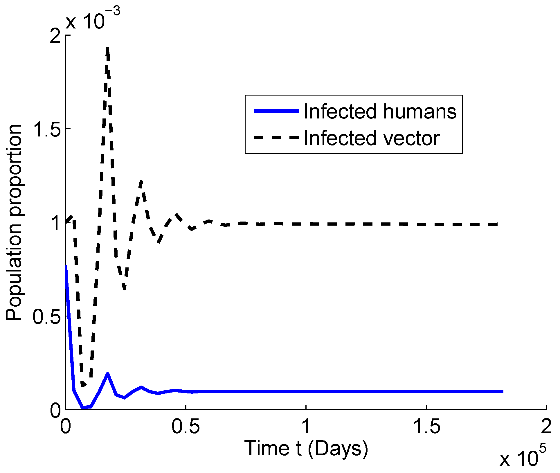
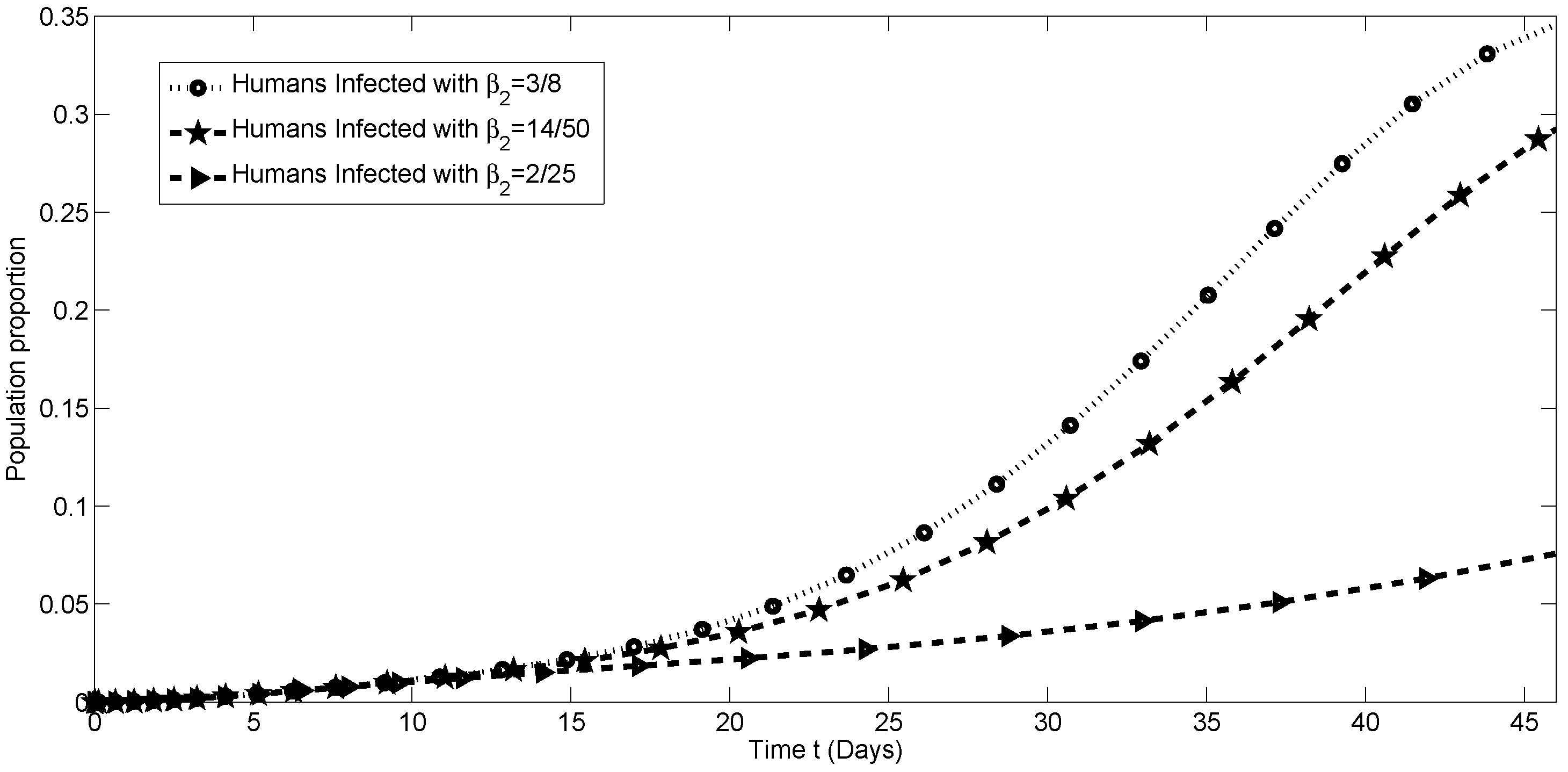
4. Numerical Simulation

In this section, a set of numerical simulations using the mathematical model of Chikungunya (2) is performed in order to support the presented theoretical results and validate the importance of the threshold parameter ${\mathcal{R}}_0$. Those simulations also help us to better understand the relationships among the different groups of the human and vector populations, the parameters, and the dynamics of Chikungunya at the population level. The numerical simulations are presented using the proportions of the subpopulations in Model (2) in order to observe easily the dynamics of Chikungunya. In addition, the simulation results are presented using the parameter values presented in

Table 1. Parameter values for mathematical model of Chikungunya (2).

Parameter	Symbol	Values	Rate
Average life-span of the human host [50]	$\frac{1}{{\mu }_h}$	25.000 Days	$0.00004$
Average life-span of the vector [51]	$\frac{1}{{\mu }_v}$	14 Days	$0.071\overline{33}$
Average incubation time of the virus (latency in the humans) [52]	$\frac{1}{\alpha }$	5–12 Days	$0.1\overline{33}$
Average incubation time of the virus (latency in the vector) [28,53]	$\frac{1}{\varphi }$	3 Days	$0.\overline{33}$
Average infection time (infection in humans) [51]	$\frac{1}{\gamma }$	5–15 Days	$0.066$
Chronic time [54,55]	$\frac{1}{\rho }$	300 Days	$0.00\overline{33}$

, which corresponds approximately to the current Colombian scenario. All simulations were done using an adaptive Runge–Kutta–Fehlberg method of order four [49].

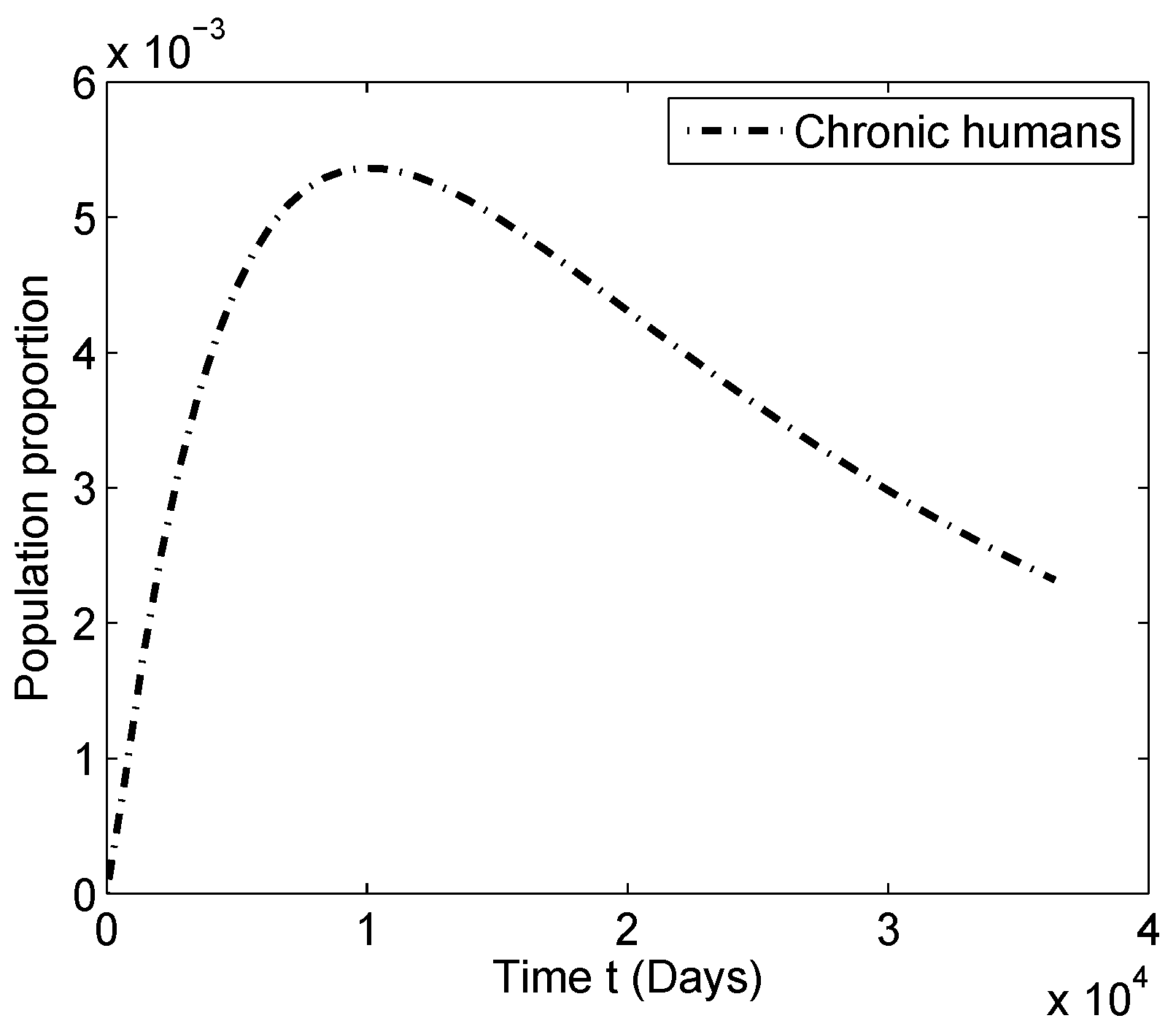
4.1. Numerical Simulations for ${\mathcal{R}}_0<1$

First, we perform numerical simulations of the Chikungunya model (2) when the threshold parameter ${\mathcal{R}}_0<1$ in order to corroborate that the infected populations vanish and to observe the dynamics of the susceptible recovered and chronic populations. We run the simulations for a time long enough so we can observe both the transient dynamics and the steady states of the system.

For this first numerical simulation, the parameter values used are those presented in Table 1, but ${\beta }_1=1/720$. In this particular scenario, the numerical value of ${\beta }_1$ is chosen such that ${\mathcal{R}}_0<1$.

As can deducted directly from the Chikungunya model (2), the units of all these parameters are in days⁻¹, except ${\beta }_i$, which measures the effective contacts per day, i.e., the total number of contacts, effective or not, per unit day, multiplied by the risk of infection with Chikungunya virus.

In Figure 2, it can be observed that for ${\mathcal{R}}_0\approx 0.93$, the infected population $I(t)$ dies out, and the susceptible population approaches the disease-free steady state value $S^d=1$. Moreover, the steady state is as expected the disease-free equilibrium $DFE=(1,0,0,0,0,1,0,0).$ In this way, if health institutions have to reduce the Chikungunya prevalence in the population, then they need to introduce changes in the health policies that affect the corresponding parameters related to ${\mathcal{R}}_0$ in order to reduce its value.

4.2. Numerical Simulations for ${\mathcal{R}}_0>1$

The second numerical simulation of the Chikungunya model (2) is when the threshold parameter ${\mathcal{R}}_0>1.$ For this particular scenario, the infected populations persist over time, as well as the susceptible and recovered populations. As in the previous scenario, we run the simulations for a time long enough so we can observe both the transient dynamics and the steady states of the system.

In Figure 3, it can be observed that for ${\mathcal{R}}_0\approx 1.1977$, the infected subpopulations $i(t)$ and $i_v(t)$ persist and approach an endemic steady state value. However, notice that despite the time-invariant parameter values, the infected subpopulations oscillate at the beginning and then reach a steady state. Thus, some slight changes of the parameter values due to environmental events may change the outcome dynamics. It is important to remark that if health institutions want to reduce the Chikungunya prevalence in the population, then they need to introduce changes in the health policies that affect the corresponding parameters related to ${\mathcal{R}}_0$ in order to reduce its value.

4.3. Sensitivity Analysis of the Transmission Parameters

Here, we investigate the relevance of each transmission parameter of the Chikungunya model (2) on the dynamics of the subpopulation of humans infected by the virus. To answer this key question, we need to compare the impact of those parameters on the outcome of the infected. As has been mentioned, the threshold parameter ${\mathcal{R}}_0$ plays a determinant role in the different subpopulations of the model.

In the previous numerical simulation, we can see in Figure 4 that varying the transmission parameter ${\beta }_2$ allows us to observe the effect of this parameter on the dynamics transmission of the disease in the human and mosquito population. In all these simulated scenarios, the human population is exposed to the mosquitoes infected by the Chikungunya virus. Based on the fact that the human population exposed to the Aedes aegypti in Colombia is 19 million [51] and assuming different values of the transmission parameter ${\beta }_2$, we can roughly estimate the number of infected humans by Chikungunya virus, as given in

Table 2. Variation of the ${\beta }_2$ parameter and its effects on the infected human population.

Value ${\mathit{\beta }}_2$	$\frac{3}{8}$	$\frac{14}{50}$	$\frac{2}{25}$
Value of ${\mathcal{R}}_0$	$4.94$	$4.27$	$2.28$
Value of Infected Population	$7.142$ million	$6.993$ million	$5.551$ million

.

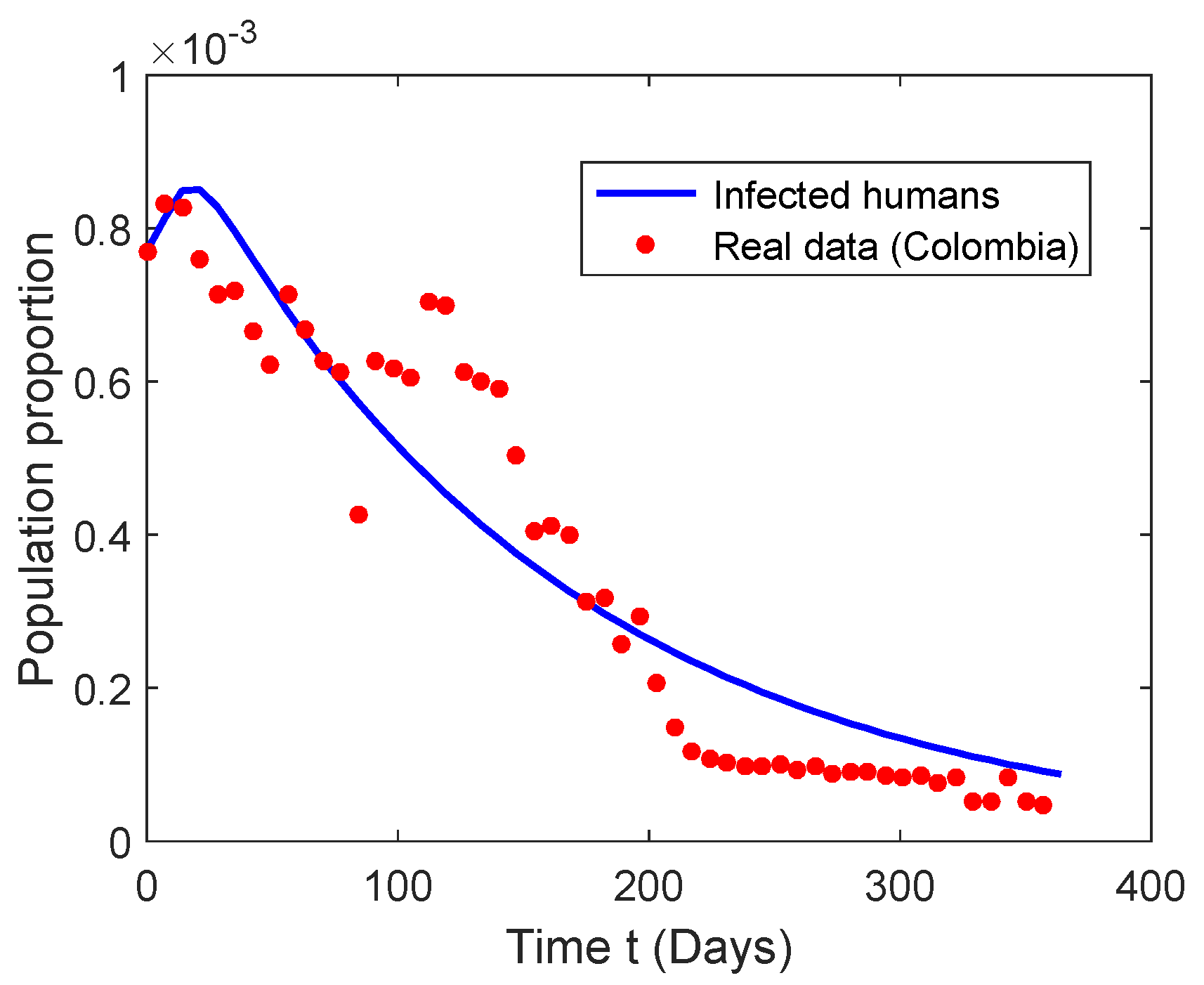
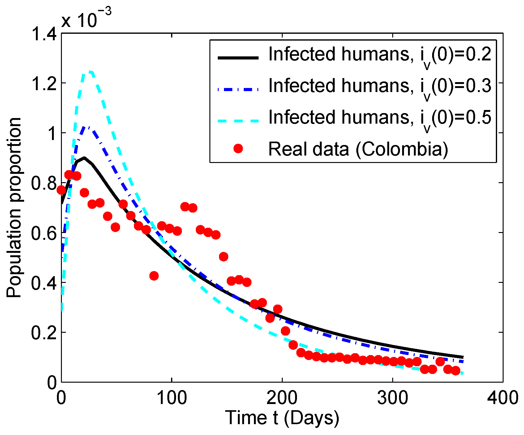
5. Estimation of Parameters for the Colombian Scenario

The dynamics of systems are, in general, too complex to allow intuitive predictions and require the support of mathematical modeling for quantitative assessments and a reliable understanding of the system functioning [56]. Moreover, one of the most difficult tasks of mathematical modeling is the estimation of model parameters.

The proposed Chikungunya mathematical model (2) establishes mathematical relationships among the eight different sub-populations and allows for the flux of individuals between sub-populations. Therefore, several parameters that regulate these relationships and fluxes appear in the model. However, the estimation of these model parameters is not a straightforward task.

5.1. Fitting Algorithm

In order to use the Chikungunya mathematical epidemiological model $()$ to simulate the dynamics of Chikungunya virus in the Colombian population, it is necessary to set the parameter values of the model. However, some of the parameter values are not accurately known or belong to different regions. Here, we rely on some parameter values that are available in scientific journals or based on medical considerations. One aim here is to explain the qualitative and quantitative behavior of the Chikungunya infection dynamics at the population level in Colombia for the year 2015.

The Chikungunya disease data were collected using available cumulative data from a national health institution in Colombia. In

Table 3. Data provided by the National Institute of Health-SIVIGILA, Colombia. The first row corresponds to the number of the week of the year 2015. The second row shows the number of infectious individuals for whom Chikungunya was detected in each week because those people went to see a doctor and it was reported.

Week	1	2	3	4	5	6	7	8
Cases	15,000	16,200	16,100	14,800	13,900	14,000	12,950	12,100
Week	9	10	11	12	13	14	15	16
Cases	13,900	13,000	12,200	11,900	8300	12,200	12,000	11,800
Week	17	18	19	20	21	22	23	24
Cases	13,700	13,600	11,900	11,700	11,500	9800	7900	8000
Week	25	26	27	28	29	30	31	32
Cases	7800	6100	6200	5000	5700	4000	2900	2300
Week	33	34	35	36	37	38	39	40
Cases	2100	2000	1900	1900	1950	1800	1900	1700
Week	41	42	43	44	45	46	47	48
Cases	1750	1750	1650	1600	1650	1500	1600	1000
Week	49	50	51	52
Cases	1000	1600	1000	900

, we can see the seroprevalence of Chikungunya infection for different weeks of 2015 in Colombia.

In order to adjust the Chikungunya mathematical model (2) to the time-series data of Chikungunya seroprevalence in Colombia, the only parameters to be estimated by a fitting process to real data are the Chikungunya transmissibility ${\beta }_1$ from infected vector to susceptible human, Chikungunya transmissibility ${\beta }_2$ from an infected human to a susceptible vector, and the initial infected human and mosquito proportions. The parameters $\beta$ depend on the number of bites per unit of time and the transmission probability per bite [57].

In regard to initial conditions for the year $2015,$ we have several assumptions due to the lack of real data for the vector and human populations. However, we think that the assumptions are biological plausible since we take into account some available data in conjunction with parameter values that are known from the related literature. As we have mentioned before, we used the proportions of the subpopulations in the Chikungunya mathematical model (2). It is important to point out that the data presented in Table 3 are related to individual cases, but we transform these data to proportional values related to the real demographic data of Colombia. We use a total population of 19,471,223, since this is the number of inhabitants that live within the 2200 m where the mosquitoes that transmit the Chikungunya virus live [51,58]. The following initial conditions based on the proportion of infected humans $i_0(i_h(0))$ are assumed: $e_0=i_0/2$ based on the fact that the latent or exposed stage is half of the infected one; $r_0=i_0/40$ based on the fact that it takes 300 days for a recovered person to start suffering chronic symptoms and with a probability of approximately $5\%$ [54,55]. Finally, we set the initial condition for the proportion of chronic individuals as $c_0=0.05\times r_0$, and the initial condition for the susceptible population is just found using the relation $s_0=1-e_0-i_0-r_0-c_0$. For the vector population, we do not have any real data. We will assume that the proportion of vectors at the eclipse phase is a tenth of the infected vectors based on the duration of the latent and infectious stages of the mosquitoes. Here, the simulation interval period of 2015 has been chosen according to the available Chikungunya seroprevalence data in Colombia.

The fitting process to adjust the Chikungunya mathematical model (2) to the time-series data of Chikungunya in Colombia corresponding to the year 2015 is done minimizing the sum of squared errors (SSR). We use two algorithms to find the minimum SSR. We initially used a genetic algorithm [59], which performs a broad search of the parameter space and is less dependent on the initial guess. Once the genetic algorithm had found a good fit, these parameters were used as the initial guess for the trust-region-reflective and interior point algorithms [60,61], which search a more localized region of the parameter space. The use of several different algorithms increases the probability of finding the global minimum for the SSR.

In order to compute the best fitting, we carried out computations, and we implemented the SSR function,

$$\begin{array}{ccccc}\mathbb{F}& :& {\mathbb{R}}^3& ⟶& \mathbb{R}\\ & & ({\beta }_1,{\beta }_2,i_v(0))& ⟶& \mathbb{F}({\beta }_1,{\beta }_2,i_v(0))\end{array}$$

where ${\beta }_1$, ${\beta }_2$, and $i_v(0)$ are variables such that:

• For a given $({\beta }_1,{\beta }_2,i_v(0))$, numerically solve the system of differential Equation (2) and obtain a solution ${\widehat{Y}}_j(t)=(\widehat{s_{hj}},\widehat{e_{hj}},\widehat{i_{hj}},\widehat{r_{hi}},\widehat{c_{hj}},\widehat{s_{vj}},\widehat{e_{vj}}$, $\widehat{i_{vj}}),$ which is an approximation of the real data solution $Y(t)$.
• Set $t_0=0$ (the fitting process starts at Week 0), and for $t=0,1,2,\dots ,51$, corresponding to weeks where data are available, evaluate the computed numerical solution for subpopulation $i_h(t)$; i.e., $\widehat{i_h}(0)$, $\widehat{i_h}(1)$, $\widehat{i_h}(2)$, …, $\widehat{i_h}(51)$.
• Compute the sum of square of the difference between $\widehat{i_h}(0)$, $\widehat{i_h}(1)$, $\widehat{i_h}(2)$, …, $\widehat{i_h}(51)$, and infectious data in Table 1. This function $\mathbb{F}$ returns the sum of squared errors ($SSR$), where for the Colombia data are given by:

  $$SSR=\sum _{j=0}^{51}{(\widehat{i_h}(j)-i_h(j))}^2$$
• Find a global minimum for the the sum of squared errors ($SSR$) using genetic, trust-region-reflective, and interior point algorithms.

The function $\mathbb{F}$ takes values in ${\mathbb{R}}^3$ and returns a positive real number, the SSR that measures the closeness of the scaled infectious population $(i_h(t)),$ provided by the model, to time-series data. In order to ensure that parameter estimates are biologically realistic, we placed bounds on some of the parameters. Thus, for instance, we can obtain values for $i_v(0)$ only from the interval $(0,1)$ or positive values for ${\beta }_1$ and ${\beta }_2$.

5.2. Numerical Simulation of the Chikungunya Mathematical Model

In this section, numerical results for the solution of the Chikungunya mathematical model (2) are presented. Since no analytic solution to the nonlinear fractional system (2) is available, we use a Runge–Kutta-type method to compute the solution numerically. The data from Colombia related to Chikungunya are from Weeks 1–52. It is important to remark that the data only show a small increasing interval for infected cases and the full decreasing interval. This is due to the fact that at the beginning of the Chikungunya epidemic, the health institutions diagnosed the cases using just symptoms instead of the lab tests that confirm a real infected case. Therefore, health institutions in Colombia disregarded most of the first increasing period in order to avoid inaccurate reports of Chikungunya. Notice that Dengue virus causes similar symptoms to the Chikungunya virus in human populations. Thus, lab tests are necessary to differentiate between both epidemics.

In order to fit the Chikungunya mathematical model (2) to the time-series data of Chikungunya cases in Colombia, we need to estimate the parameters ${\beta }_1$, ${\beta }_2$, and $i_v(0)$. As a first approach, we set the initial proportion of latent and infected humans based on the real data. Thus, we only need to estimate initially ${\beta }_1$, ${\beta }_2$, and $i_v(0)$. In other works, different assumptions regarding the initial infected and latent populations for humans and vectors have been assumed. For instance, in [62], the authors assumed that the initial numbers of latent and infectious people were equal, and analogously for the mosquito population.

The confirmed cases of Chikungunya from the year 2015 in Colombia and the best model fit along with the best fit parameter values are shown in Figure 5. It can be seen graphically that the Chikungunya mathematical model (2) produces a good adjustment to the real data and predicts that the epidemic will disappear in Colombia due to a ${\mathcal{R}}_0=0.79$. In addition, the epidemic peak of the mathematical model approximates well the peak of the real data. It is important to mention that the Chikungunya mathematical model (2) generates epidemic data that fit well in terms of the SSR. The Chikungunya mathematical model (2) gives a smoother curve due to its deterministic nature, as was expected. In order to catch the natural irregularity of the real data, it would be necessary to introduce stochastic factors to the model, which allows one to obtain a more accurate fitting [63]. However, introducing stochastic or temporal factors would require more detailed information regarding the dynamics of the population in Colombia, and the complexity of the model would increase. It is important to mention that the irregularity of the real data has been observed in many other studies related to other diseases, and can be explained due to different reasons such as weather, under-reporting, the stochastic nature of the virus diffusion, spatial effects, or even the heterogeneity of the human and mosquito population [19]. In Figure 6, the long-term dynamics of the humans with chronic rheumatoid symptoms can be observed. It can be seen that this class population will reach a peak and then start to decrease due to the natural death rate and the decay of new infected humans over the long term.

Additionally, we considered different scenarios fixing the initial conditions for the mosquito infected population $i_v(0)$ and fitting the initial infected human population $i_h(0)$. However, the most important difference with the previous best fit scenario is that the values of the parameters ${\beta }_2$ and ${\beta }_1$ varied in such way that they compensated each other in order to be able to fit the real data level of infected humans. This compensation makes total sense since the transmission parameters ${\beta }_s$ are going to depend on the initial infected vector population $i_v(0)$. The smaller $i_v(0)$ is, the greater should be the transmission parameter from vector to humans in order to reproduce the real number of infected cases. However, we notice that the basic reproduction number ${\mathcal{R}}_0$ stays approximately constant for all the scenarios. Thus, from the results, we obtained a robust numerical value for the basic reproduction number ${\mathcal{R}}_0$, regardless of the initial proportion of infected mosquitoes.

Finally, we present the numerical simulations for larger values of $i_v(0)$. We vary $i_v(0)$ from 0.2 (20%) to 0.5 (50%) in order to observe other potential realistic scenarios. The idea is to test hypotheses that consider larger values for the initial proportion of infected vectors $i_v(0)$. The best model fits can be seen in Figure 7. It can be observed graphically that the mathematical model (2) does not fit the real data well for large values of $i_v(0)$. Based on these results and the real data available, we can infer that these large value scenarios are unlikely for Colombia in 2015. Moreover, notice that for larger values of the initial proportion of infected vectors $i_v(0)$, the model fits to the real data deteriorate. Thus, we have highlighted some likely scenarios for the parameter values of ${\beta }_1$, ${\beta }_2$, $i_v(0)$, and $i_0$ that can help to analyze some potential scenarios beyond the data and with some intervention strategies. Moreover, this allows us to compare with different regions where other parameter values have been obtained and then raise some questions regarding the explanations of these differences. In the next section, we will provide further analysis regarding the identifiability of the parameters, the initial conditions, and the basic reproduction number ${\mathcal{R}}_0$.

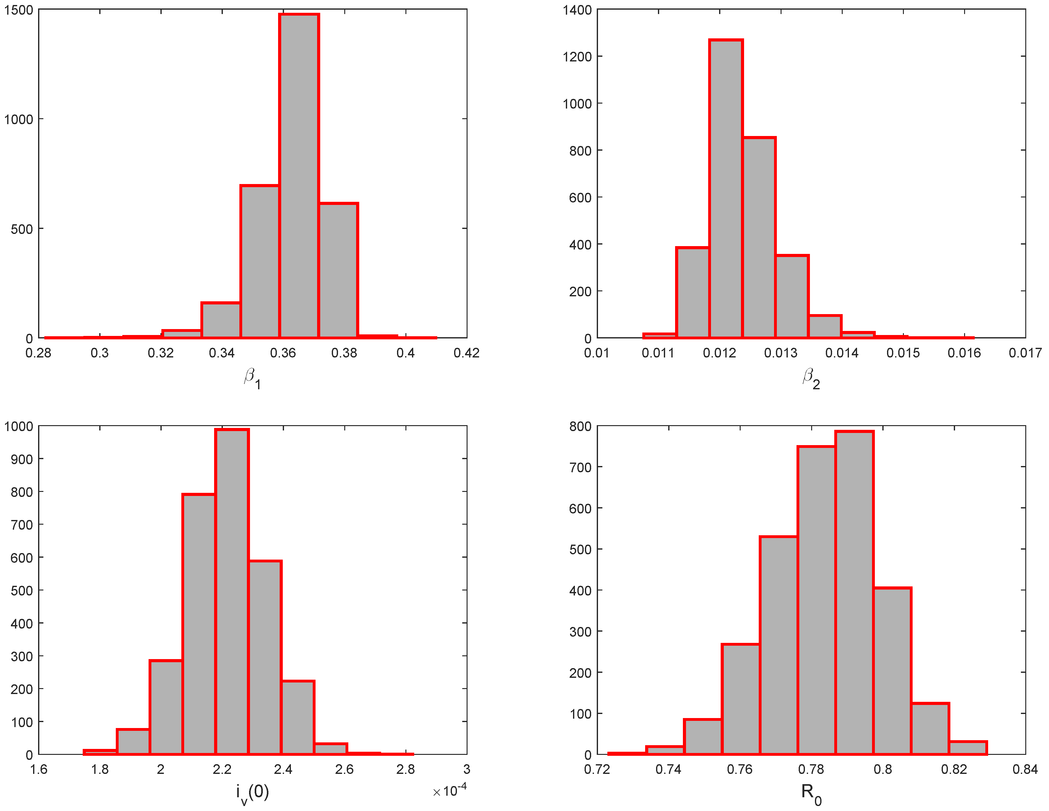
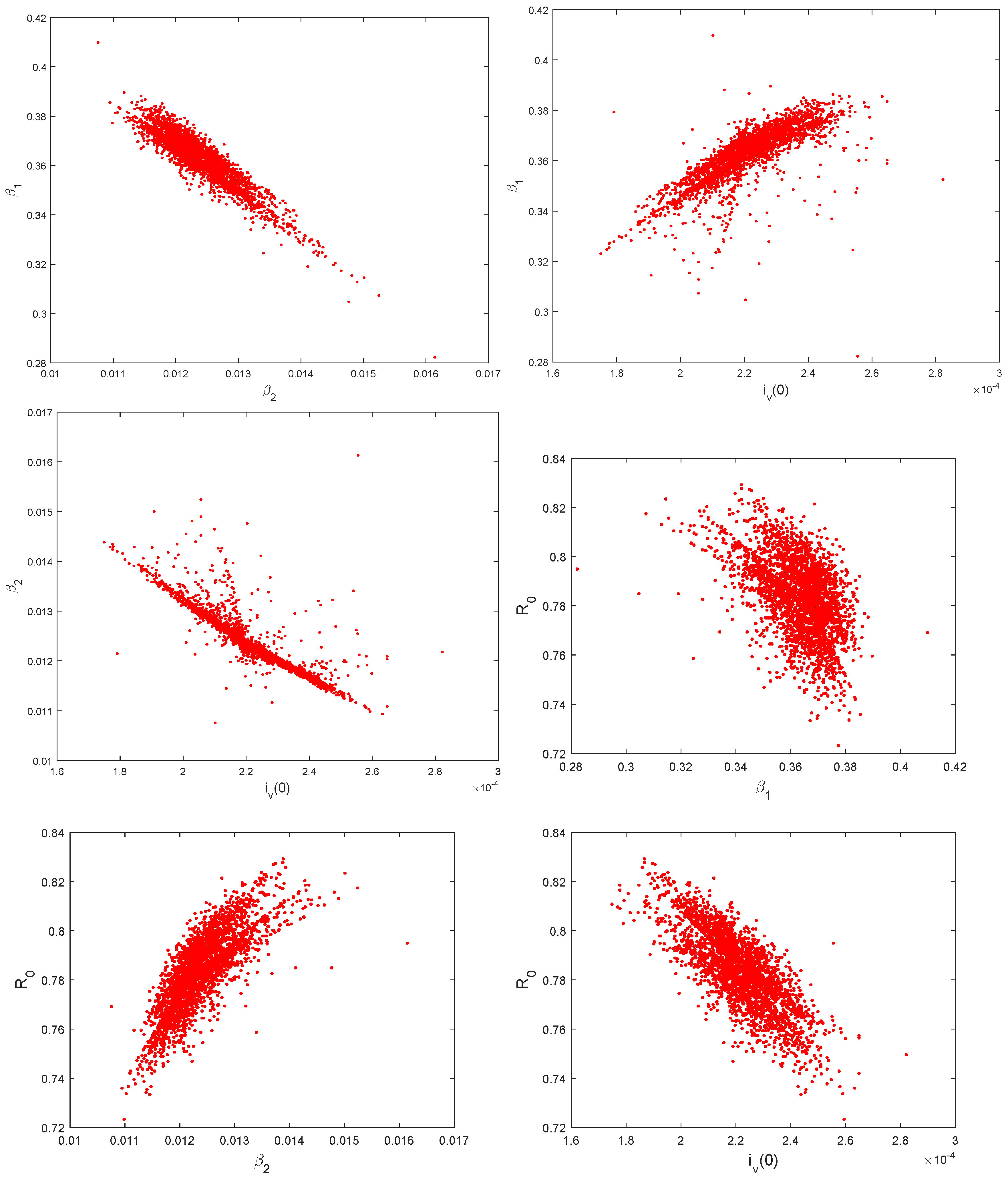
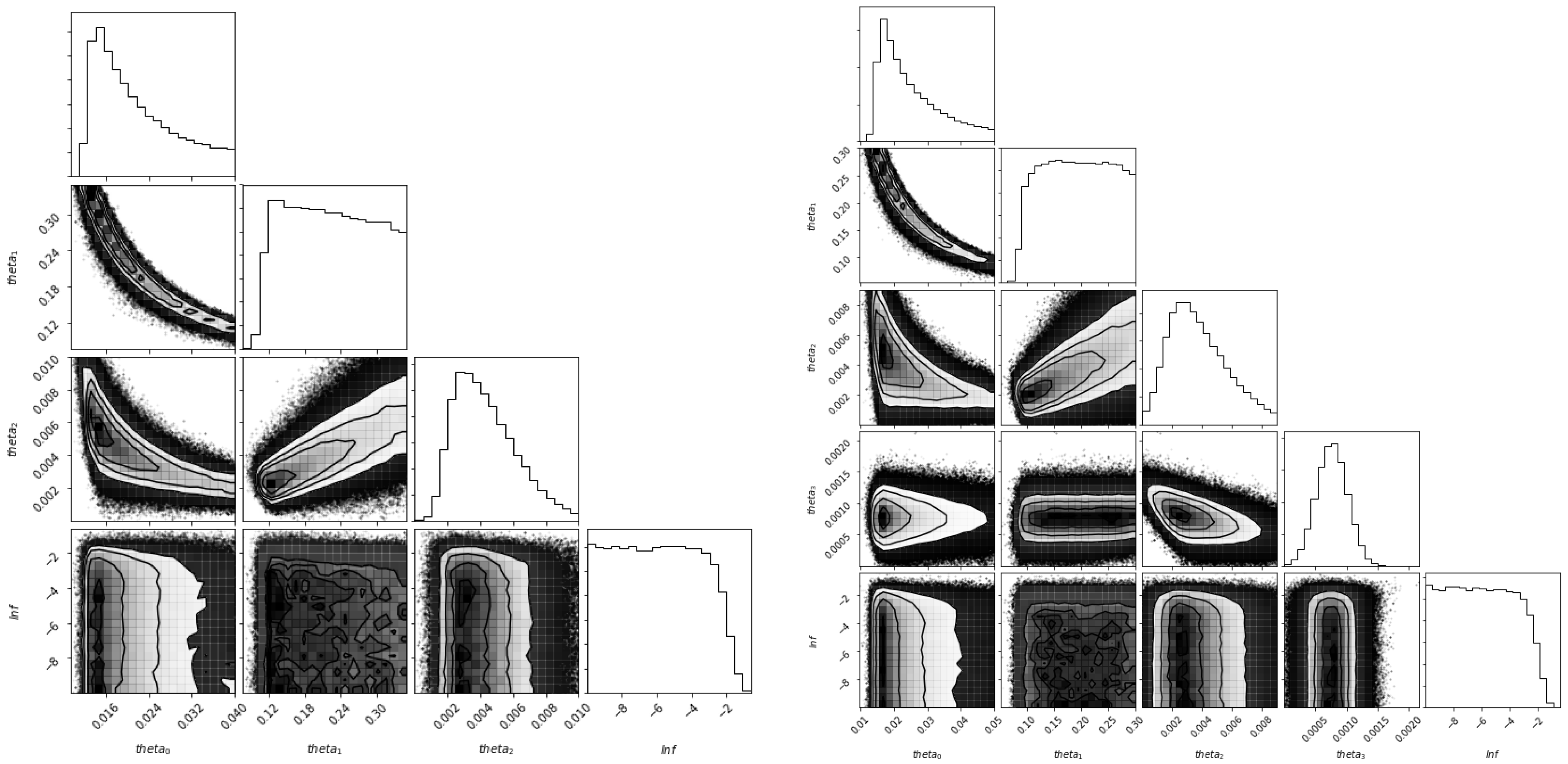
5.3. Identifiability of the Parameters

As we mentioned before, the parameters ${\beta }_1$ and ${\beta }_2$ are not fully identifiable. Moreover, we do not have real data regarding initial conditions for the different subpopulations, but based on our assumptions, all of them can be set in terms of the initial conditions for the infected human and vector populations. Here, we use two approaches: for the first one, we fixed the initial condition of the infected humans to the real data, and consequently, we minimized the function $\mathbb{F}$ in ${\mathbb{R}}^3$; the second approach was just to leave the initial condition of infected humans as a parameter, and then, we minimized the function $\mathbb{F}$ in ${\mathbb{R}}^4.$

We now extend our parameters’ identifiability analysis, by incorporating two numerical techniques. These techniques are bootstrapping [34,64] and Markov chain Monte Carlo [35,36,39], which allow us to introduce further information regarding the identifiability of the parameters and corroborate the identifiability of the basic reproduction number ${\mathcal{R}}_0$. It is recommended to ensure that the optimum parameter values of the model can be uniquely determined by the available real data. For non-linear-based models, the issue of identifiability is not straightforward.

An important numerical tool often used to assess the uncertainty in estimated values is bootstrapping [34,64]. The bootstrapping process begins with the generation of artificially-generated datasets, which are created by sampling the best fit curve and adding error such that the SSR is equal to the SSR of the original data. The mathematical model (2) is fitted to each of the surrogated datasets, leading to new parameter estimates. A total of 3000 bootstrap replicates were performed using the real data. In this way, we obtained estimates of the distribution of each parameter, as can be seen in Figure 8. Roughly, it can be seen from the histograms that all the parameter estimates follow a Gaussian distribution. These distributions were used to give the 95% confidence intervals, which are shown in

Table 4. Estimated parameters using the mathematical model (2) and the prevalence data of Chikungunya in the population of Colombia in the year 2016.

Parameters	${\mathcal{R}}_0$	${\mathit{i}}_{\mathit{v}}(0)$
Values	0.78 (0.74–0.84)	2.18 ${\times 10}^{-4}$ (1.95 ${\times 10}^{-4}$–2.45 ${\times 10}^{-4})$
Parameters	${\beta }_1$	${\beta }_2$
Values	0.36 (0.34–0.38)	0.012 (0.011–0.13)

The 95% confidence intervals (bootstrap fits) are given in parentheses.

. This information is useful to have a measure of error in the parameter estimates. There is some small skew present in the histograms of parameters $T_h$ and $T_M,$ which can be explained by their correlation. However, we are more interested in the threshold parameter ${\mathcal{R}}_0$, which as can be seen in Figure 9, is relatively stable around ${\mathcal{R}}_0=0.78$.

The bootstrapping method allows us to find correlations between estimated parameters. In Figure 9, several two-parameter scatter plots for each of the 3000 bootstrap replicates can be observed. In order to have two uncorrelated parameters, the scatter plot should be roughly a circle, with no clear relationship between the two parameters. For the parameter $i_v(0)$, the plots show a little bit of correlation, and this was in some way expected since $i_v(0)$ is a factor on how strongly the epidemic starts. There is a clear correlation between the transmission parameters ${\beta }_1$ and ${\beta }_2$. This correlation in some way is expected since both transmission parameters are related to the exposure of humans to mosquitoes and vice versa. However, it is important to remark that we are more interested in their product since the epidemic threshold parameter ${\mathcal{R}}_0$ is proportional to this product. These results suggest that the threshold parameter ${\mathcal{R}}_0$ of the mathematical model (2) is identifiable. Thus, we can use the model with caution to describe the dynamics of the spread of Chikungunya in the population of Colombia in the year 2016.

The second numerical technique is based on Markov chain Monte Carlo [35,36]. In particular, we used a stable algorithm of the affine-invariant ensemble sampler for Markov chain Monte Carlo (MCMC) proposed in [65]. An algorithm that is affine invariant performs equally well under all linear transformations; it will therefore be insensitive to covariances among parameters [66]. Markov chain Monte Carlo is designed to sample from—and thereby provide sampling approximations to–the posterior PDF efficiently [35,66]. In the algorithm that is used here, we draw samples from a multivariate Gaussian density. It is necessary to set up the specific values of the hyperparameters in three dimensions (${\beta }_1,{\beta }_2$, $i_v(0)$). In addition, we need to decide how many walkers there are, which are in some way independent paths to reach the maximum of the likelihood function [65]. There are different options to initialize each of the walkers. One of the best techniques is to start in a small ball around the a priori preferred position [66]. It is important to mention that the walkers will spread out and explore the whole space for the parameters. The main goal is to find the maximum of the likelihood function, which is a Gaussian where the variance is underestimated by some fractional amount. We can use Markov Chain Monte Carlo to obtain estimates and confidence intervals for each of the parameters ${\beta }_1,{\beta }_2$, and $i_v(0)$. Moreover, we can observe some possible correlations among the parameters.

In Figure 10, all the one- and two-dimensional projections of the posterior probability distributions of the parameters can be seen. This allows us to observe all of the covariances between parameters. In addition, the histograms show the marginalized distribution for a parameter or a set of parameters using the results of Markov chain Monte Carlo. Thus, Figure 10 shows the marginalized distribution for each parameter independently in the histograms along the diagonal and then the marginalized two-dimensional distributions in the other panels [66]. Notice that the maximum likelihood function profile is also presented. We can say that in order to have two uncorrelated parameters, the level curves’ plot should be close to circles, with no clear relationship between the two parameters. For the parameter $i_v(0)$, the plots show less correlation in comparison with the ones with respect to ${\beta }_1$ and ${\beta }_2$, and this was in some way expected since $i_v(0)$ is a factor of how strongly the epidemic starts. There is a clear correlation between the transmission parameters ${\beta }_1$ and ${\beta }_2$, as we also observed with the bootstrapping results. In fact, this relationship has the same pattern. This correlation in some way is expected since both transmission parameters are related to the exposure of humans to mosquitoes and vice versa. However, it is important to remark that we are more interested in their product since the epidemic threshold parameter ${\mathcal{R}}_0$ is proportional to this product, as we have mentioned before. These results agree with previous results regarding identifiability for epidemic models with vectors [67].

6. Conclusions

We present a mathematical model of the spread of the Chikungunya disease at the population level that incorporates the transmission vector by including cross-transmission between the human and vector populations. The proposed model includes a chronic subpopulation, which to the best of our knowledge has not been considered in other mathematical models. We determined the epidemic threshold parameter ${\mathcal{R}}_0$ for the extinction of disease using the method of the next generation matrix. Using Lyapunov function theory, some sufficient conditions for the global stability of the the disease-free equilibrium were obtained. Based on this parameter, we found the parameters that affect the basic reproduction number ${\mathcal{R}}_0$ and therefore what would be the best policies to control the spread of the Chikungunya disease. We verified that when the threshold parameter ${\mathcal{R}}_0$ is less than unity, the disease disappears, while when threshold parameter values are larger than one, the disease persists in the population. Numerical simulations were presented to support the established theoretical results.

Using the proposed mathematical model of Chikungunya diffusion, we were able to analyze the dynamics of infection during the 2015 outbreak in Colombia. In particular, we estimated the numerical values of the epidemiological parameters ${\beta }_1$, ${\beta }_2$, and the reproduction number ${\mathcal{R}}_0$. Based on numerical results of the model of Chikungunya, we were able to better explain and understand the variation of the number of infected cases with the Chikungunya virus in Colombia. We found that the transmission parameters ${\beta }_1$ and ${\beta }_2$ were highly correlated.

Our estimated values for the reproduction number ${\mathcal{R}}_0$ ranged from $0.74$–$0.84$ across the three different scenarios proposed and also from the results of bootstrapping and Markov chain Monte Carlo methods. However, notice that rain seasons have been changing recently due to climate change, and that could affect some of the parameter values, which is one limitation of this model. The fitting of the model to the observed weekly reports during the 2015 outbreak in Colombia is relatively good, despite the natural irregularity of the real data. This irregularity of the data has been observed in many other studies related to other diseases and can be due to different reasons such as weather, under-reporting, the stochastic nature of the virus diffusion, spatial effects, or even the heterogeneity of the human and mosquito population. All these factors were not considered here explicitly and are other limitations of this work. Other limitations are the fact that the initial proportion of the different subpopulations is unknown. More complex models are necessary to study all the aforementioned factors, and future works might consider these factors or at least some of them. Another important aspect that we found in this study, based on the previous numerical simulations of the different scenarios, is that the initial infected population of mosquitoes is likely no greater than $20\%$ for the year 2015 in Colombia. To the best of our knowledge, we do not know if there are real data regarding this particular description.

In this paper, we performed identifiability analysis in order to estimate some parameters of the model and found correlations among the parameters of the model. We used the bootstrapping technique and Markov chain Monte Carlo in order to assess the identifiability of the parameters of the model. We found out that the parameters were not fully identifiable with the prevalence of the real data that we had. However, we were able to identify that the reproduction number ${\mathcal{R}}_0$ ranged from 0.74–0.84. It is important to notice that this result depends on some fixed parameter values such as the duration of the infectious stage and the life-span of the mosquitoes. Changing values for these parameters can change the aforementioned range for the reproduction number ${\mathcal{R}}_0$. However, regardless of some potential changes, we presented a study with a methodology to deal with these types of epidemic models when real data are available.

Finally, we can conclude that in order to reduce the Chikungunya disease diffusion, it is important first to decrease the transmission parameters. For instance, people could use clothes covering most of the body to avoid mosquito bits and could also use repellents. Any action that could reduce the infected mosquitoes’ bites will affect the reproduction number ${\mathcal{R}}_0$. The aforementioned actions would reduce the transmission of the virus in both directions. Another way to reduce the value of the reproduction number ${\mathcal{R}}_0$ is to increase the mortality of the mosquito population. Therefore, a health policy that could be implemented is to increase this mortality. Other parameters that are included in ${\mathcal{R}}_0$ such as incubation or infected period are natural characteristics of the Chikungunya virus and are difficult to modify.

References

1. Zárate, M.L. Arbovirus y Arbovirosis en México. Instituto de Salubridad y Enfermedades Tropicales. Available online: www.fmvz.unam.mx/fmvz/cienciavet/revistas-/CVvol2/CVv2c6.pdf (accessed on 2 January 2019).
2. Jupp, P.; McIntosh, B. Chikungunya virus disease. In The Arboviruses: Epidemiology and Ecology; CRC Press: Boca Raton, FL, USA, 1988; Volume 2, pp. 137–157. [Google Scholar]
3. Pérez Sánchez, G.; Ramírez Alvarez, G.; Pérez Gijón, Y.; Canela Lluch, C. Fiebre de Chikungunya: Enfermedad infrecuente como emergencia médica en Cuba. Medisan 2014, 18, 848–856. [Google Scholar]
4. Cook, G.C.; Zumla, A. Manson’s Tropical Diseases, 13th ed.; Elsevier Health Sciences: Philadelfia, PA, USA, 2008. [Google Scholar]
5. Benedict, M.; Levine, R.; Hawley, W.; Lounibos, P. Spread of the tiger: Global risk of invasion by the mosquito Aedes albopictus. Vector Borne Zoonotic Dis. 2007, 7, 76–85. [Google Scholar] [CrossRef] [PubMed]
6. Robinson, M.; Conan, A.; Duong, V.; Ly, S.; Ngan, C.; Buchy, P.; Tarantola, A.; Rodo, X. A model for a chikungunya outbreak in a rural Cambodian setting: Implications for disease control in uninfected areas. PLoS Negl. Trop. Dis. 2014, 8, e3120. [Google Scholar] [CrossRef] [PubMed]
7. Charrel, R.N.; De Lamballerie, X.; Raoult, D. Seasonality of mosquitoes and chikungunya in Italy. Lancet Infect. Dis. 2008, 8, 5–6. [Google Scholar] [CrossRef]
8. Halstead, S.B. Reappearance of chikungunya, formerly called dengue, in the Americas. Emerg. Infect. Dis. 2015, 21, 557–561. [Google Scholar] [CrossRef]
9. Teng, T.S.; Kam, Y.W.; Lee, B.; Hapuarachchi, H.C.; Wimal, A.; Ng, L.C.; Ng, L.F. A systematic meta-analysis of immune signatures in patients with acute chikungunya virus infection. J. Infect. Dis. 2015, 211, 1925–1935. [Google Scholar] [CrossRef] [PubMed]
10. Sissoko, D.; Malvy, D.; Ezzedine, K.; Renault, P.; Moscetti, F.; Ledrans, M.; Pierre, V. Post-epidemic Chikungunya disease on Reunion Island: Course of rheumatic manifestations and associated factors over a 15-month period. PLoS Negl. Trop. Dis. 2009, 3, e389. [Google Scholar] [CrossRef]
11. Montero, A. Chikungunya fever—A new global threat. Med. Clín. (Eng. Ed.) 2015, 145, 118–123. [Google Scholar] [CrossRef]
12. Poo, Y.S.; Rudd, P.A.; Gardner, J.; Wilson, J.A.; Larcher, T.; Colle, M.A.; Le, T.T.; Nakaya, H.I.; Warrilow, D.; Allcock, R.; et al. Multiple immune factors are involved in controlling acute and chronic chikungunya virus infection. PLoS Negl. Trop. Dis. 2014, 8, e3354. [Google Scholar] [CrossRef]
13. Taubitz, W.; Cramer, J.P.; Kapaun, A.; Pfeffer, M.; Drosten, C.; Dobler, G.; Burchard, G.D.; Löscher, T. Chikungunya fever in travelers: Clinical presentation and course. Clin. Infect. Dis. 2007, 45, e1–e4. [Google Scholar] [CrossRef]
14. García, G.; Santana, E.; Martínez, J.R.; Álvarez, A.; Rodríguez, R.; Guzmán, M.G. Detección de respuesta linfoproliferativa en monos inoculados con virus dengue 4. Rev. Cubana Med. Trop. 2003, 55, 27–29. [Google Scholar] [PubMed]
15. Manore, C.A.; Ostfeld, R.S.; Agusto, F.B.; Gaff, H.; LaDeau, S.L. Defining the risk of Zika and chikungunya virus transmission in human population centers of the eastern United States. PLoS Negl. Trop. Dis. 2017, 11, e0005255. [Google Scholar] [CrossRef] [PubMed]
16. Murray, J.D. Mathematical Biology I: An Introduction, Vol. 17 of Interdisciplinary Applied Mathematics; Springer: New York, NY, USA, 2002. [Google Scholar]
17. Castillo-Chavez, C.; Brauer, F. Mathematical Models in Population Biology and Epidemiology; Springer: New York, NY, USA, 2012. [Google Scholar]
18. Hethcote, H.W. Mathematics of infectious diseases. SIAM Rev. 2005, 42, 599–653. [Google Scholar] [CrossRef]
19. González-Parra, G.; Arenas, A.J.; Aranda, D.F.; Segovia, L. Modeling the epidemic waves of AH1N1/09 influenza around the world. Spat. Spatio-Temporal Epidemiol. 2011, 2, 219–226. [Google Scholar] [CrossRef] [PubMed]
20. Lashari, A.A.; Hattaf, K.; Zaman, G. A delay differential equation model of a vector borne disease with direct transmission. Int. J. Ecol. Econ. Stat. 2012, 27, 25–35. [Google Scholar]
21. Lashari, A.A.; Hattaf, K.; Zaman, G.; Li, X.Z. Backward bifurcation and optimal control of a vector borne disease. Appl. Math. Inf. Sci. 2013, 7, 301–309. [Google Scholar] [CrossRef]
22. Ullah, S.; Khan, M.A.; Farooq, M. A fractional model for the dynamics of TB virus. Chaos Solitons Fractals 2018, 116, 63–71. [Google Scholar] [CrossRef]
23. Sardar, T.; Rana, S.; Bhattacharya, S.; Al-Khaled, K.; Chattopadhyay, J. A generic model for a single strain mosquito-transmitted disease with memory on the host and the vector. Math. Biosci. 2015, 263, 18–36. [Google Scholar] [CrossRef]
24. Wojtak, W.; Silva, C.J.; Torres, D.F. Uniform asymptotic stability of a fractional tuberculosis model. Math. Model. Nat. Phenom. 2018, 13, 9. [Google Scholar] [CrossRef] [Green Version]
25. Yakob, L.; Clements, A.C. A mathematical model of chikungunya dynamics and control: The major epidemic on Réunion Island. PLoS ONE 2013, 8, e57448. [Google Scholar] [CrossRef]
26. Agusto, F.B.; Easley, S.; Freeman, K.; Thomas, M. Mathematical Model of Three Age-Structured Transmission Dynamics of Chikungunya Virus. Comput. Math. Methods Med. 2016, 2016, 4320514. [Google Scholar] [CrossRef]
27. Lashari, A.A.; Zaman, G. Global dynamics of vector-borne diseases with horizontal transmission in host population. Comput. Math. Appl. 2011, 61, 745–754. [Google Scholar] [CrossRef] [Green Version]
28. Dumont, Y.; Chiroleu, F.; Domerg, C. On a temporal model for the Chikungunya disease: Modeling, theory and numerics. Math. Biosci. 2008, 213, 80–91. [Google Scholar] [CrossRef] [PubMed]
29. Moulay, D.; Aziz-Alaoui, M.; Cadivel, M. The chikungunya disease: Modeling, vector and transmission global dynamics. Math. Biosci. 2011, 229, 50–63. [Google Scholar] [CrossRef] [PubMed]
30. Sawabe, K.; Isawa, H.; Hoshino, K.; Sasaki, T.; Roychoudhury, S.; Higa, Y.; Kasai, S.; Tsuda, Y.; Nishiumi, I.; Hisai, N.; et al. Host-feeding habits of Culex pipiens and Aedes albopictus (Diptera: Culicidae) collected at the urban and suburban residential areas of Japan. J. Med. Entomol. 2010, 47, 442–450. [Google Scholar] [CrossRef]
31. Vourc’h, G.; Halos, L.; Desvars, A.; Boué, F.; Pascal, M.; Lecollinet, S.; Zientara, S.; Duval, T.; Nzonza, A.; Brémont, M. Chikungunya antibodies detected in non-human primates and rats in three Indian Ocean islands after the 2006 ChikV outbreak. Vet. Res. 2014, 45, 52. [Google Scholar] [CrossRef] [PubMed] [Green Version]
32. Ligon, B.L. Reemergence of an unusual disease: The chikungunya epidemic. Semin. Pediatr. Infect. Dis. 2006, 17, 99–104. [Google Scholar] [CrossRef] [PubMed]
33. Diallo, M.; Thonnon, J.; Traore-Lamizana, M.; Fontenille, D. Vectors of Chikungunya virus in Senegal: Current data and transmission cycles. Am. J. Trop. Med. Hyg. 1999, 60, 281–286. [Google Scholar] [CrossRef]
34. Efron, B. Bootstrap Methods: Another Look at the Jackknife. Ann. Stat. 1979, 7, 1–26. [Google Scholar] [CrossRef]
35. MacKay, D.J.; Mac Kay, D.J. Information Theory, Inference and Learning Algorithms; Cambridge University Press: Cambridge, UK, 2003. [Google Scholar]
36. Tulu, T.W.; Tian, B.; Wu, Z. Mathematical modeling, analysis and Markov Chain Monte Carlo simulation of Ebola epidemics. Res. Phys. 2017, 7, 962–968. [Google Scholar] [CrossRef]
37. Dhamala, J.; Arevalo, H.J.; Sapp, J.; Horácek, B.M.; Wu, K.C.; Trayanova, N.A.; Wang, L. Quantifying the uncertainty in model parameters using Gaussian process-based Markov chain Monte Carlo in cardiac electrophysiology. Med. Image Anal. 2018, 48, 43–57. [Google Scholar] [CrossRef] [PubMed]
38. Kroese, D.P.; Brereton, T.; Taimre, T.; Botev, Z.I. Why the Monte Carlo method is so important today. Wiley Interdiscip. Rev. Comput. Stat. 2014, 6, 386–392. [Google Scholar] [CrossRef]
39. Bretó, C. Modeling and inference for infectious disease dynamics: A likelihood-based approach. Stat. Sci. 2018, 33, 57–69. [Google Scholar]
40. Ortiz, G.A.; Alvarez, D.A.; Bedoya-Ruíz, D. Identification of Bouc–Wen type models using the transitional Markov chain Monte Carlo method. Comput. Struct. 2015, 146, 252–269. [Google Scholar] [CrossRef]
41. Weber, C. Characterization of the Chikungunya Virus Entry Process and The Development of Novel Antiviral Strategies. Ph.D. Thesis, Univ.-Bibliothek Frankfurt am Main, Frankfurt, Germany, 2015. [Google Scholar]
42. Arenas, A.J.; González-Parra, G.; Moraño, J.A. Stochastic modeling of the transmission of respiratory syncytial virus (RSV) in the region of Valencia, Spain. Biosystems 2009, 96, 206–212. [Google Scholar] [CrossRef] [PubMed]
43. Van den Driessche, P.; Watmough, J. Reproduction numbers and sub-threshold endemic equilibria for compartmental models of disease transmission. Math. Biosci. 2002, 180, 29–48. [Google Scholar] [CrossRef]
44. Diekmann, O.; Heesterbeek, J.A.P.; Roberts, M. The construction of next-generation matrices for compartmental epidemic models. J. R. Soc. Interface 2010, 7, 873–885. [Google Scholar] [CrossRef] [Green Version]
45. Guerrero, F.; González-Parra, G.; Arenas, A.J. A nonstandard finite difference numerical scheme applied to a mathematical model of the prevalence of smoking in Spain: A case study. Comput. Appl. Math. 2014, 33, 13–25. [Google Scholar] [CrossRef]
46. Van den Driessche, P.; Watmough, J. Further notes on the basic reproduction number. In Mathematical Epidemiology; Springer: New York, NY, USA, 2008; pp. 159–178. [Google Scholar]
47. Korobeinikov, A.; Maini, P.K. A Lyapunov function and global properties for SIR and SEIR epidemiological models with nonlinear incidence. Math. Biosci. Eng. 2004, 1, 57–60. [Google Scholar]
48. Shuai, Z.; van den Driessche, P. Global stability of infectious disease models using Lyapunov functions. SIAM J. Appl. Math. 2013, 73, 1513–1532. [Google Scholar] [CrossRef]
49. Kincaid, D.R.; Cheney, E.W. Numerical Analysis: Mathematics of Scientific Computing; American Mathematical Soc.: Providence, RI, USA, 2002; Volume 2. [Google Scholar]
50. Duque, J.E.; Navarro-Silva, M.A. Simulating management of Aedes aegypti (Diptera: Culicidae) and its effects in a dengue epidemic. Revista Colombiana de Entomología 2009, 35, 66–72. [Google Scholar]
51. Cardona-Ospina, J.A.; Henao-SanMartin, V.; Paniz-Mondolfi, A.E.; Rodríguez-Morales, A.J. Mortality and fatality due to Chikungunya virus infection in Colombia. J. Clin. Virol. 2015, 70, 14–15. [Google Scholar] [CrossRef] [PubMed]
52. Vazeille, M.; Moutailler, S.; Coudrier, D.; Rousseaux, C.; Khun, H.; Huerre, M.; Thiria, J.; Dehecq, J.S.; Fontenille, D.; Schuffenecker, I.; et al. Two Chikungunya isolates from the outbreak of La Reunion (Indian Ocean) exhibit different patterns of infection in the mosquito, Aedes albopictus. PLoS ONE 2007, 2, e1168. [Google Scholar] [CrossRef] [PubMed]
53. Chikaki, E.; Ishikawa, H. A dengue transmission model in Thailand considering sequential infections with all four serotypes. J. Infect. Dev. Countries 2009, 3, 711–722. [Google Scholar] [CrossRef]
54. Gutierrez, M.F. Personal Communication. 2017. [Google Scholar]
55. Plan Nacional de Respuesta Frente a la Introducción del Virus de Chikungunya en Colombia. Available online: https://www.minsalud.gov.co (accessed on 2 January 2019).
56. Chou, I.C.; Voit, E.O. Recent developments in parameter estimation and structure identification of biochemical and genomic systems. Math. Biosci. 2009, 219, 57–83. [Google Scholar] [CrossRef] [PubMed] [Green Version]
57. Cruz-Pacheco, G.; Esteva, L.; Vargas, C. Control measures for Chagas disease. Math. Biosci. 2012, 237, 49–60. [Google Scholar] [CrossRef] [PubMed]
58. Censo Colombia 2005. Available online: https://www.dane.gov.co/files/censos/libroCenso2005nacional.pdf (accessed on 2 January 2019).
59. Golberg, D.E. Genetic Algorithms in Search, Optimization, and Machine Learning; Addion Wesley: Boston, MA, USA, 1989. [Google Scholar]
60. Coleman, T.F.; Li, Y. An Interior Trust Region Approach for Nonlinear Minimization Subject to Bounds. SIAM J. Optim. 1996, 6, 418–445. [Google Scholar] [CrossRef] [Green Version]
61. Press, W.H.; Teukolsky, S.A.; Vetterling, W.T.; Flannery, B.P. Numerical Recipes: The Art of Scientific Computing; Cambridge University Press: Cambridge, UK, 1992. [Google Scholar]
62. Kucharski, A.J.; Funk, S.; Eggo, R.M.; Mallet, H.P.; Edmunds, W.J.; Nilles, E.J. Transmission dynamics of Zika virus in island populations: A modelling analysis of the 2013–14 French Polynesia outbreak. PLoS Negl. Trop. Dis. 2016, 10, e0004726. [Google Scholar] [CrossRef]
63. González-Parra, G.; Villanueva, R.J.; Ruiz-Baragaño, J.; Moraño, J.A. Modelling influenza A(H1N1) 2009 epidemics using a random network in a distributed computing environment. Acta Trop. 2015, 143, 29–35. [Google Scholar] [CrossRef] [Green Version]
64. Davison, A.C.; Hinkley, D.V. Bootstrap Methods and Their Application; Cambridge University Press: Cambridge, UK, 1997; Volume 1. [Google Scholar]
65. Goodman, J.; Weare, J. Ensemble samplers with affine invariance. Commun. Appl. Math. Comput. Sci. 2010, 5, 65–80. [Google Scholar] [CrossRef] [Green Version]
66. Foreman-Mackey, D.; Hogg, D.W.; Lang, D.; Goodman, J. emcee: The MCMC hammer. Publ. Astron. Soc. Pac. 2013, 125, 306. [Google Scholar] [CrossRef]
67. Kao, Y.H.; Eisenberg, M.C. Practical unidentifiability of a simple vector-borne disease model: Implications for parameter estimation and intervention assessment. Epidemics 2018, 25, 89–100. [Google Scholar] [CrossRef] [PubMed]
Figure 1. Dynamics of the Chikungunya virus with transmission vector. The boxes represent the subpopulation and the arrows the transition between the subpopulations. Arrows are labeled by their corresponding model parameters.
Mca 24 00006 g001
Figure 2. Numerical simulation of the Chikungunya model (2) when the threshold parameter R 0 = 0.987 . The parameter values are those presented in Table 1, but β 1 = 1 / 720 .
Mca 24 00006 g002
Figure 3. Numerical simulation of the Chikungunya model (2) when the threshold parameter R 0 = 1.1977 . The parameter values are those presented in Table 1, but β 1 = 1 / 600 .
Mca 24 00006 g003
Figure 4. The dynamics of the different subpopulations are sensitive to the changes of the parameter β 2 .
Mca 24 00006 g004
Figure 5. Best fit of the Chikungunya mathematical model (2) to the time-series data of Chikungunya in Colombia corresponding to the year 2015. Red points give the real data, and the blue line shows the best model fit. The best fit parameter values are given in the table. SSR, sum of squared errors.
Mca 24 00006 g005
Parameter β 1 β 2 i v ( 0 ) SSR R 0
Value 0.361 0.0122.186 × 10−44.701 × 10−70.77
Figure 6. Dynamic of the chronic infected individual humans using the fit of the Chikungunya mathematical model (2) to the time-series data of Chikungunya in Colombia corresponding to the year 2015.
Mca 24 00006 g006
Figure 7. Best fits of the Chikungunya mathematical model (2) to the time-series data of Chikungunya in Colombia corresponding to the year 2015. The initial proportion of infected vectors i v ( 0 ) varies from 0.2 (20%) to 0.5 (50%).
Mca 24 00006 g007
Figure 8. Identifiability assessment of the mathematical model (2) fit to the prevalence data of Chikungunya in the population of Colombia in the year 2016. Correlation plots generated with parameter estimates from bootstrap fits.
Mca 24 00006 g008
Figure 9. Identifiability assessment of the mathematical model (2) fit to the prevalence data of Chikungunya in the population of Colombia in the year 2016. Correlation plots generated with parameter estimates from bootstrap fits. Correlation between the parameters β 1 , β 2 , i M ( 0 ) , and R 0 .
Mca 24 00006 g009
Figure 10. Identifiability assessment of the mathematical model (2) fit to the prevalence data of Chikungunya in the population of Colombia in the year 2016. Correlation plots generated with Markov chain Monte Carlo for three ( β 1 , β 2 , i v ( 0 ) ) and four parameters ( β 1 , β 2 , i v ( 0 ) , i h ( 0 ) ), respectively.
Mca 24 00006 g010