Spectral Element Method Modeling of Eddy Current Losses in High-Frequency Transformers


Abstract
:1. Introduction
2. Modeling Approach
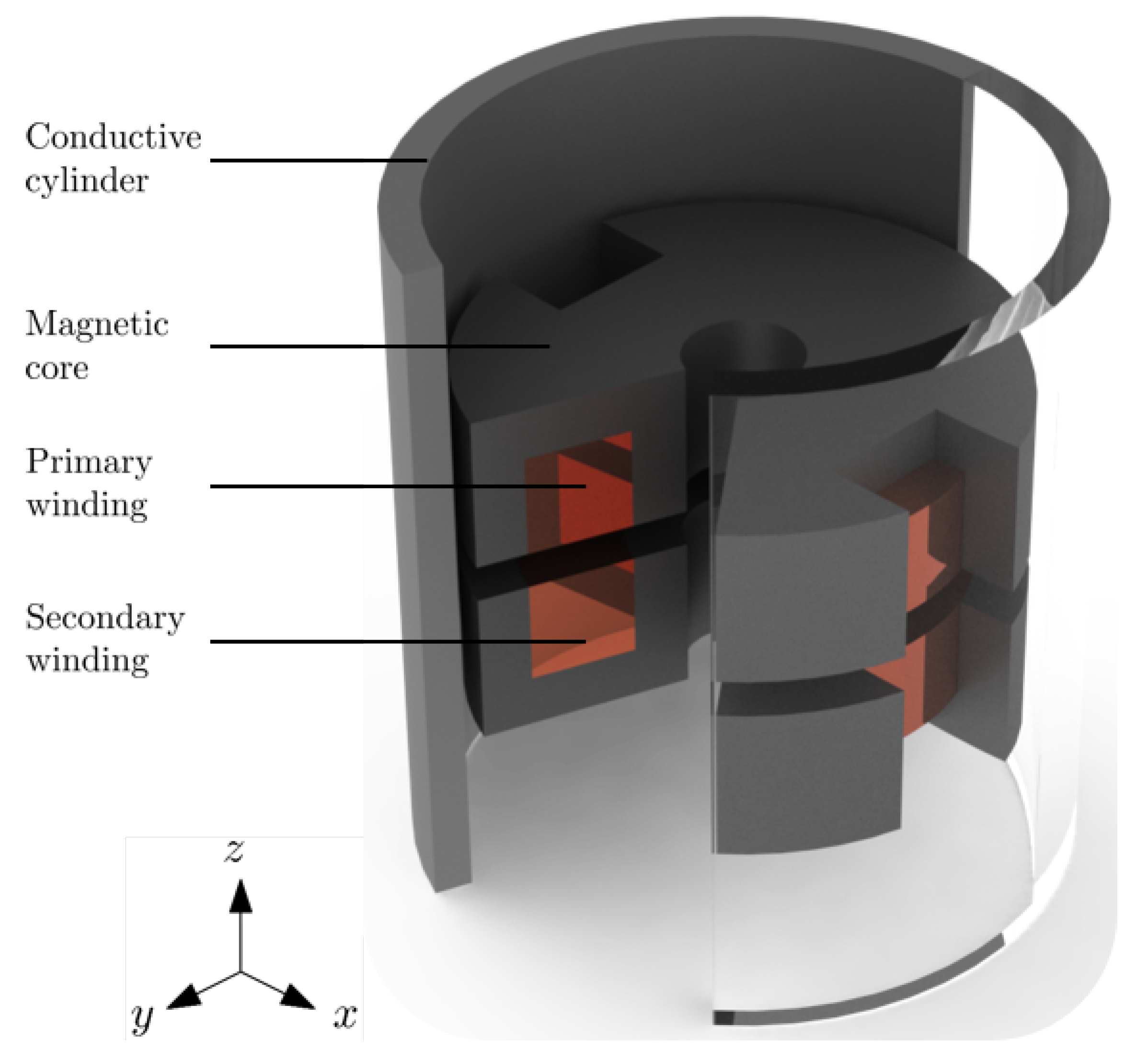
3. Benchmark System
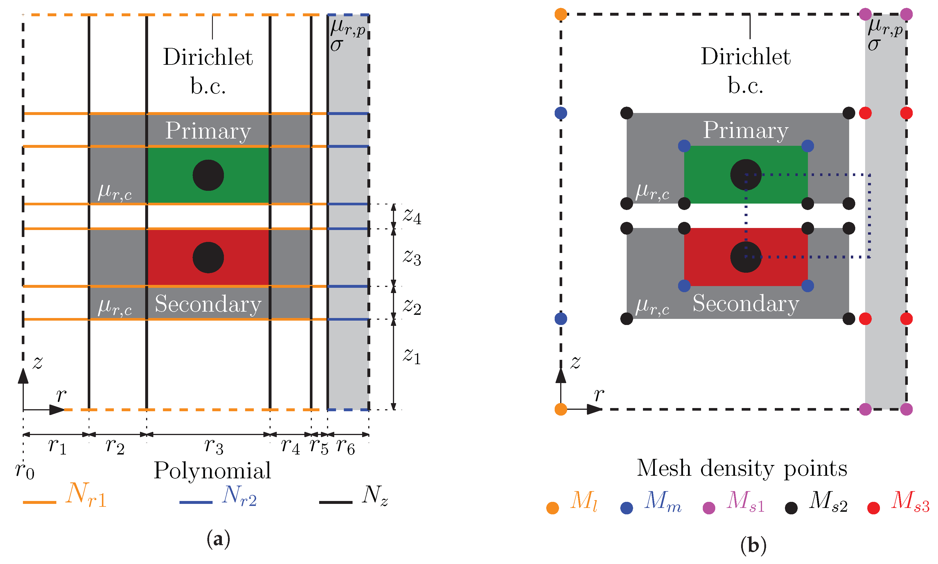
3.1. SEM Model
3.2. FEM Model
3.3. Assumptions
4. Convergence Analysis and Refinement Optimization
5. Results
6. Conclusions
Author Contributions
Conflicts of Interest
References
- Kazmierkowski, M.P.; Moradewicz, A.; Duarte, J.; Lomonova, E.; Sonntag, C. Contactless Energy Transfer. In Power Electronics and Motor Drives, 2nd ed.; Wilamowski, B., Irwin, J., Eds.; CRC Press: Boca Rotan, FL, USA, 2011; Chapter 35; pp. 1–17. [Google Scholar]
- Qian, W.; Zhang, X.; Fu, Y.; Lu, J.; Bai, H. Applying normally-off GaN HEMTs for coreless high-frequency wireless chargers. CES Trans. Electr. Mach. Syst. 2017, 1, 418–427. [Google Scholar]
- Choi, J.; Tsukiyama, D.; Tsuruda, Y.; Davila, J.M.R. High-Frequency, High-Power Resonant Inverter with eGaN FET for Wireless Power Transfer. IEEE Trans. Power Electron. 2018, 33, 1890–1896. [Google Scholar] [CrossRef]
- Boughrara, K.; Dubas, F.; Ibtiouen, R. 2-D Analytical Prediction of Eddy Currents, Circuit Model Parameters, and Steady-State Performances in Solid Rotor Induction Motors. IEEE Trans. Magn. 2014, 50, 1–14. [Google Scholar] [CrossRef]
- De Gersem, H. Spectral-element method for high-speed rotating cylinders. COMPEL 2009, 28, 730–740. [Google Scholar] [CrossRef]
- Gilson, A.; Tavernier, S.; Dubas, F.; Depernet, D.; Espanet, C. 2-D analytical subdomain model for high-speed permanent-magnet machines. In Proceedings of the 18th International Conference on Electrical Machines and Systems (ICEMS), Pattaya, Thailand, 25–28 October 2015; pp. 1508–1514. [Google Scholar]
- Hariri, A.O.; Youssef, T.; Elsayed, A.; Mohammed, O. A Computational Approach for a Wireless Power Transfer Link Design Optimization Considering Electromagnetic Compatibility. IEEE Trans. Magn. 2016, 52, 1–4. [Google Scholar] [CrossRef]
- Peralta, A.; Alizad, S.H.; Alam, N.; Singh, V. On the use of eddy currents to facilitate wireless power transfer through metallic surfaces. In Proceedings of the 2017 IEEE Wireless Power Transfer Conference (WPTC), Taipei, Taiwan, 10–12 May 2017; pp. 1–4. [Google Scholar]
- Plasser, R.; Koczka, G.; Bíró, O. Improvement of the Finite-Element Analysis of 3-D, Nonlinear, Periodic Eddy Current Problems Involving Voltage-Driven Coils under DC Bias. IEEE Trans. Magn. 2018, 54, 1–4. [Google Scholar] [CrossRef]
- Curti, M.; van Beek, T.A.; Jansen, J.W.; Gysen, B.L.J.; Lomonova, E.A. General Formulation of the Magnetostatic Field and Temperature Distribution in Electrical Machines Using Spectral Element Analysis. IEEE Trans. Magn. 2018, 54, 1–9. [Google Scholar] [CrossRef]
- Patera, A.T. A spectral element method for fluid dynamics: Laminar flow in a channel expansion. J. Comput. Phys. 1984, 54, 468–488. [Google Scholar] [CrossRef]
- Lee, J.H.; Xiao, T.; Liu, Q.H. A 3-D spectral-element method using mixed-order curl conforming vector basis functions for electromagnetic fields. IEEE Trans. Microw. Theory Tech. 2006, 54, 437–444. [Google Scholar]
- Curti, M.; Paulides, J.J.H.; Lomonova, E.A. Magnetic Modeling of a Linear Synchronous Machine With the Spectral Element Method. IEEE Trans. Magn. 2017, 53, 1–6. [Google Scholar] [CrossRef]
- De Gersem, H. Combined Spectral-Element, Finite-Element Discretization for Magnetic-Brake Simulation. IEEE Trans. Magn. 2010, 46, 3520–3523. [Google Scholar] [CrossRef]
- Zanella, R.; Nore, C.; Bouillault, F.; Cappanera, L.; Tomas, I.; Mininger, X.; Guermond, J. Study of Magnetoconvection Impact on a Coil Cooling by Ferrofluid with a Spectral/Finite-Element Method. IEEE Trans. Magn. 2018, 54, 1–4. [Google Scholar] [CrossRef]
- Kopriva, D.A. Implementing Spectral Methods for Partial Differential Equations; Springer Science + Business Media B.V.: Dordrecht, The Netherlands, 2009. [Google Scholar]
- Alonso, A.; Valli, A. Eddy Current Approximation of Maxwell Equations; Springer Science + Business Media B.V.: Milan, Italy, 2010. [Google Scholar]
- Touzani, R.; Rappaz, J. Mathematical Models for Eddy Currents and Magnetostatics; Springer Science + Business Media B.V.: Dordrecht, The Netherlands, 2014. [Google Scholar]
- Kriezis, E.E.; Tsiboukis, T.D.; Panas, S.M.; Tegopoulos, J.A. Eddy currents: Theory and applications. Proc. IEEE 1992, 80, 1559–1589. [Google Scholar] [CrossRef]
- Komatitsch, D.; Vilotte, J.P.; Vai, R.; Castillo-Covarrubias, J.M.; Sánchez-Sesma, F.J. The spectral element method for elastic wave equations—Application to 2-D and 3-D seismic problems. Int. J. Numer. Methods Eng. 1999, 45, 1139–1164. [Google Scholar] [CrossRef]
- Lee, J.H.; Liu, Q.H. An efficient 3-D spectral-element method for Schrödinger equation in nanodevice simulation. IEEE Trans. Comput. Aided Des. Integr. Circuits Syst. 2005, 24, 1848–1858. [Google Scholar]
- Bastiaens, K.; Krop, D.C.J.; Jumayev, S.; Lomonova, E.A. Design and Comparison of High-Frequency Resonant and Non-Resonant Rotating Transformers. In Proceedings of the 21st International Conference on Electrical Machines and Systems (ICEMS), Jeju, Korea, 7–10 October 2018; pp. 1703–1708. [Google Scholar]
- Henrotte, F.; Hedia, H.; Bamps, N.; Genon, A.; Nicolet, A.; Legros, W. A new method for axisymmetrical linear and nonlinear problems. IEEE Trans. Magn. 1993, 29, 1352–1355. [Google Scholar] [CrossRef]
- User Guide Flux 2018.1. Available online: https://altairhyperworks.com/product/flux (accessed on 21 February 2019).


| Geometrical Parameters | |||
| Parameter | Symbol | Value | Unit |
| Geometry offset radius | 0.10 | mm | |
| Radial thickness of the inner air region | 1.55 | mm | |
| Radial thickness of the inner core leg | 1.45 | mm | |
| Radial thickness of the winding area | 2.80 | mm | |
| Radial thickness of the outer core leg | 1.35 | mm | |
| Radial thickness of the air gap | 0.50 | mm | |
| Full radial thickness of the conductive cylinder | 1.00 | mm | |
| Modeled radial thickness of the conductive cylinder | 52.2 | m | |
| Height air region | 4.55 | mm | |
| Core height | 1.40 | mm | |
| Winding area height | 2.80 | mm | |
| Air gap height | 1.00 | mm | |
| Physical Quantities | |||
| Quantity | Symbol | Value | Unit |
| Frequency | f | 1.0 | MHz |
| Plate conductivity | 8.41 | S/m | |
| Plate relative permeability | 100 | - | |
| Skin depth | 17.4 | m | |
| Core relative permeability | 3000 | - | |
| Primary current density | 4.21 | A/mm | |
| Secondary current density | 1.35 | A/mm | |
| Phase primary current | |||
| Phase secondary current | 159.8 | ||
| SEM Discretization (p-refinement) | ||||
| Polynomial | Symbol | Minimum (-) | Maximum (-) | Steps (-) |
| Radial 1 | 1 | 10 | 10 | |
| Radial 2 | 1 | 30 | 30 | |
| Axial | 1 | 30 | 30 | |
| FEM Discretization (h-refinement) | ||||
| Mesh point | Symbol | Minimum (mm) | Maximum (mm) | Steps (-) |
| Large | 1.00 | 3.00 | 7 | |
| Medium | 0.40 | 1.00 | 7 | |
| Small 1 | 0.10 | 1.00 | 7 | |
| Small 2 | 0.10 | 1.00 | 10 | |
| Small 3 | 0.10 | 1.00 | 10 | |
| Converged Solution | ||||
| Method | Losses (W) | d.o.f. (-) | Relative Error (%) | Time (s) |
| FEM (reference) | 5.0848 | 2.7504 × 10 | 0.0000 | 5.701 |
| FEM | 5.0848 | 1.7117 × 10 | 7.0071 × 10 | 4.731 |
| SEM | 5.0848 | 6.4770 × 10 | 7.0076 × 10 | 1.418 |
| Pareto Optimum 1 | ||||
| FEM | 5.0790 | 2.9230 × 10 | 0.1140 | 4.875 |
| SEM | 5.1213 | 2.2500 × 10 | 0.7182 | 4.015 × 10 |
| Pareto Optimum 2 | ||||
| FEM | 5.0805 | 3.4400 × 10 | 8.374 × 10 | 3.198 |
| SEM | 5.0812 | 7.0400 × 10 | 7.081 × 10 | 5.807 × 10 |
| SEM Discretization (p-refinement) | |||
| Polynomial | Symbol | Pareto Optimum 1 (-) | Pareto Optimum 2 (-) |
| Radial 1 | 2 | 5 | |
| Radial 2 | 4 | 6 | |
| Axial | 2 | 3 | |
| FEM Discretization (h-refinement) | |||
| Mesh Point | Symbol | Pareto Optimum 1 (mm) | Pareto Optimum 2 (mm) |
| Large | 3.00 | 2.00 | |
| Medium | 0.80 | 0.70 | |
| Small 1 | 1.00 | 0.85 | |
| Small 2 | 0.30 | 0.30 | |
| Small 3 | 0.90 | 0.80 | |
© 2019 by the authors. Licensee MDPI, Basel, Switzerland. This article is an open access article distributed under the terms and conditions of the Creative Commons Attribution (CC BY) license (http://creativecommons.org/licenses/by/4.0/).
Share and Cite
Bastiaens, K.; Curti, M.; Krop, D.C.J.; Jumayev, S.; Lomonova, E.A. Spectral Element Method Modeling of Eddy Current Losses in High-Frequency Transformers. Math. Comput. Appl. 2019, 24, 28. https://doi.org/10.3390/mca24010028
Bastiaens K, Curti M, Krop DCJ, Jumayev S, Lomonova EA. Spectral Element Method Modeling of Eddy Current Losses in High-Frequency Transformers. Mathematical and Computational Applications. 2019; 24(1):28. https://doi.org/10.3390/mca24010028
Chicago/Turabian StyleBastiaens, Koen, Mitrofan Curti, Dave C. J. Krop, Sultan Jumayev, and Elena A. Lomonova. 2019. "Spectral Element Method Modeling of Eddy Current Losses in High-Frequency Transformers" Mathematical and Computational Applications 24, no. 1: 28. https://doi.org/10.3390/mca24010028
APA StyleBastiaens, K., Curti, M., Krop, D. C. J., Jumayev, S., & Lomonova, E. A. (2019). Spectral Element Method Modeling of Eddy Current Losses in High-Frequency Transformers. Mathematical and Computational Applications, 24(1), 28. https://doi.org/10.3390/mca24010028