A Mathematical Model for Intimate Partner Violence

Abstract

In the context of mathematical models applied to social sciences, we present and analyze a model based on differential equations for the intimate partner violence (IPV). Such a model describes the dynamics of a heterosexual romantic couple in which the man perpetrates violence against the woman. We focus on incorporating different key factors reported in the literature as causal or motivational factors to perpetrate IPV. Among the main factors included are the failures in self-regulation, the man’s need to control the woman, the social pressure on the woman to remain married, and empowerment programs. Another aspect that we include is periodic alcohol consumption for the man. The discussion of the model includes a stability analysis of its equilibrium points and the asymptotic behavior of its solutions. Also, the interpretation of results is presented in terms of IPV phenomenon. Finally, a brief review is given on different scales to quantify human behavioral traits and numerical simulations for some IPV scenarios.

1. Introduction

Violence against woman is a social problem that afflicts all societies, without distinction of race, socioeconomic level or academic degree. In fact, it is considered a global public health problem by the World Health Organization (WHO), due to its frequency and alarming consequences of violence against women. In particular, the intimate partner violence (IPV) is one of the most common and includes physical, sexual or emotional abuse by the intimate partner towards the woman, according to WHO [1]. Paradoxically, this type of violence is also usually one of the most forgiven, quiet and ignored, often for being something that occurs in privacy and is perpetrated by the loved one. Although IPV is officially penalized and rejected, it continues to occur with relative impunity, and is sometimes well accepted by some societies. Global statistics estimate that about one out of three women have experienced some type of violence worldwide. In Mexico, six out of ten women have been victims of some kind of aggression, at least once in their lives, and four out of ten have suffered some type of violence caused by her intimate partner. Likewise, 33% of the women in Mexico suffered violence during childhood and seven femicides occur daily according to the statistics of the National Institute of Statistics and Geography (INEGI) [2]. Worldwide, Mexico ranks 71 of 169 countries ranked according to their gender inequality measured with the Gender Inequality Index (GII) [3,4]. From our point of view, these statistics show the importance of studying this problem. However, mathematical modeling involving differential equations is an approach almost not used in social science problems, but it has proven its importance to understand and offer a solution for different problems [5,6,7].

The classical approach of mathematics in social sciences usually involves the application of statistical techniques. A common situation is the validation of hypothesis through statistical tests. Another application of statistical models is the measurement and quantification of different factors or variables. As an example of quantification of the level of violence, we can refer to [8] by Sánchez et al. where a study to measure the level of historical violence of a population is described. Our approach is different from these examples. We search for models to describe the evolution in time of violence or related variables. With this approach, we find models such as the one reported by Poza et al. [9] which is an epidemiological type model that describes the evolution of the populations of different types of men, who were classified according to their level of woman abuse in Spain. This model is in terms of difference equations and predicts the evolution of IPV in Spain based on the statistical information reported by the literature. Another, important and pioneer work which is supported by a long and deep research on human behavior for marital couples is reported in [10,11] by Gottman et al. Let us say, that this article is not directly related to violence levels, but it presents and analyzes a model to predict a possible marital dissolution. In fact, it succeeded remarkably well. The model considers two functions of “influence” which aim to model the balance of positive-negative attitudes of a spouse towards the other in the context of an interview on conflict topics. The talk is recorded and coded according to a validated scale to obtain the parameters of the model. Using this information the authors were capable of making predictions on marriage success chances. We borrow some ideas of this article to model the interaction between the intimate partners involved in a violent relationship which we will discuss later.

On the other side, let us describe some sociological and psychological theories related to violence which we will use to construct our model. It is important to mention that sociologists have studied and analyzed this serious problem and developed a number of different theories. For example in [12], L. Walkers points out that violence against women is a cyclic process that consists of an accumulation of stress, acute violence, and reconciliation. Also, that this behavior has its origin in the patriarchal culture, which is enmeshed in the men’s and women’s thoughts through social learning mechanisms. Moreover, in the context of a patriarchal society, the success of a man in a relationship is based on the use of power and control of the woman, according to Corsi [13]. Another work also in the context of social learning theory which we found useful is the article by Stith and Fairley [14]. There, the authors propose a statistical model to predict violence in the couple, taking external and internal variables of the man. They reported that sex-role egalitarianism, approval, and observation of marital violence have effects on the use of severe marital violence. Moreover, that the observation of marital violence decreases self-esteem which raises marital stress and the level of alcohol consumption, both of which may increase marital violence. However, they remark that egalitarianism has a negative effect on the violence level, meaning, it could decrease the use of severe violence. Otherwise, those violent acts damage the self-esteem of the woman and create codependency toward her intimate partner which could be boosted by social pressure. On the opposite side, we take into account the effect of empowerment programs for the woman which have proven to be an effective strategy to reduce IPV [15], and we will include it as an external factor that could change the violence dynamic in a couple.

Finally, Finkel et al. [16] have reported that self-regulatory failures are important predictors of IPV. Besides that, the self-regulation capacity of a battering man is a trait that can be improved or depleted through training sessions. From the above and from various sociological multiple causal models, we will consider causal and motivational factors in our study. The causal factors are those that set the “perfect scenario” for male violence to occur in a relationship, this is according to the social learning theory. The causal factors in the man that unleash violence are the following: Violence observed during childhood, low self- esteem, acceptance of machismo, and failures in self-regulation. On the other hand, the motivational factors are those that motivate to perpetrate the violence and are more likely to trigger a violent episode in the relationship. The motivational factors that we will consider are the man’s need to control woman and the effect of external factors for the woman. Other facts that support our selection of factors that we will include in the model come from the Mexican national surveys on violence [2,17]. There, violence against women is described and fits the situation that our model intends to simulate. Let us remark that health-related factors such as mental and/or physical illnesses and external support factors such as psychological therapies will not be considered in our proposed model.

Our objective is to model mathematically the dynamics of the IPV problem in one couple in order to contribute to a better understanding of this social phenomenon. Let us remark that while violence affects both men and women, the violence against women is more alarming in some countries, for example in Mexico. For this reason, our model describes violence in one direction, man battering woman. This model was proposed using the theory of differential equations and taking into account causes or relevant factors that may contribute to the triggering of the violent behavior described above. We present the development of a first mathematical model in ordinary differential equations, which allows us to predict the possible violent situations that a woman could face in the relationship. Later, we use the obtained model to simulate computationally probable scenarios of violence.

The article is organized as follows: In Section 2 we present and explain the assumptions made in order to construct the model in differential equations. In particular, in Section 2.1 we present a simple model without considering the interaction between the romantic partners, as we do in Section 2.2. In Section 2.3. we discuss different scales related to the variables and parameters of our model. While in Section 3, we present the asymptotic analysis of the model without considering the man’s alcohol consumption and provide its interpretation in terms of the factors considered. In Section 4, we show numerical simulations for some IPV scenarios. Later in Section 5, a discussion about the model and its application is given. Finally, conclusions are presented in the last section.

2. Mathematical Modeling

Our aim is to give a model that describes the IPV dynamics in a romantic couple. In order to explain in detail the model formation, let us present it in two parts. In the first one, we consider equations for each spouse independently of their intimate partner. We will call this interaction non-influenced intimate partner interaction. In the second one, we include the interaction between intimate partners. We call it influenced intimate partner interaction.

2.1. Non-influenced Intimate Partner Interaction

Let us first define two variables, one for the man and the other for the women. The variable $v\left(t\right)$ is the man’s violent behavior index (positive) at time t which indicates the potential level of the man’s hostility or aggression. The variable $i\left(t\right)$ is the woman independence behavior index which indicates the woman’s state of freedom (positive) or potential of dependency or submission (negative).

• A0. In a similar way and following [10], we assume the existence of non-influenced steady states $\tilde{v}$ and $\tilde{i}$ for each individual, man and woman indexes, respectively. Those states are independent of each other intimate partner. Actually, they depend on their own personal history with respect to the IPV problem. For this reason, we assume that the non-influenced steady states are directly proportional to two causal factors: Violence seen in childhood and acceptance of violence. So, we define the non-influenced man’s violence steady state as $\tilde{v}={\alpha }_1{\beta }_1$ and the non-influenced woman’s independence steady state as $\tilde{i}=(1-{\alpha }_2)(1-{\beta }_2),$ where ${\alpha }_1,{\alpha }_2$ are the parameters that quantify the violence watched in childhood for man and woman, respectively, and ${\beta }_1,{\beta }_2$ are the parameters that quantify the acceptance of machismo for the man and woman, respectively. Notice that the non-influenced independence index of the woman decreases according to the level of violence watched during her infancy and her acceptance of IPV [18]. We will discuss these parameters in more detail in the next section.
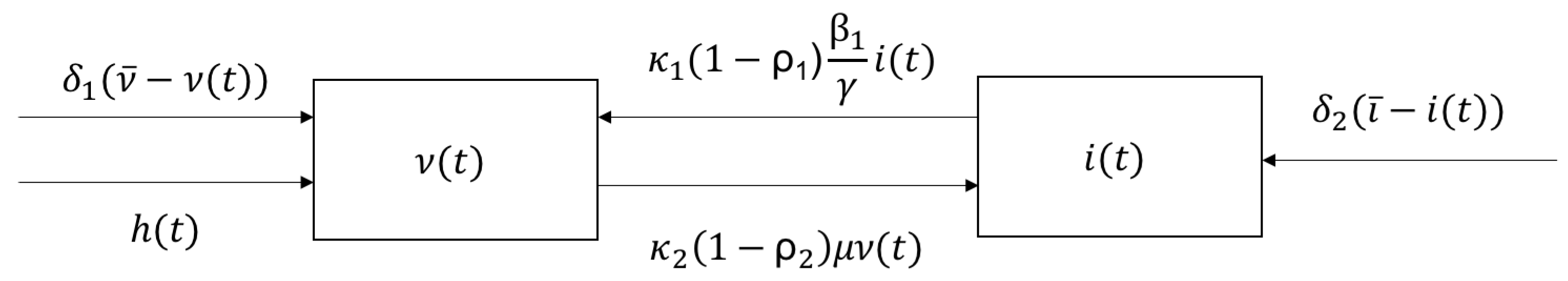
• A1. These non-influenced steady states correspond to an equilibrium point $(\tilde{v},\tilde{i})$ of the following differential equation system:

  $$\begin{array}{cc}\frac{dv\left(t\right)}{dt}& ={\delta }_1(\tilde{v}-v\left(t\right)),v\left(0\right)=v_0,\\ \frac{di\left(t\right)}{dt}& ={\delta }_2(\tilde{i}-i\left(t\right)),i\left(0\right)=i_0,\end{array}$$

  (1)

  where ${\delta }_1$ and ${\delta }_2$ are positive constant called “inertias” which are associated with the coping abilities with the problems of each individual of the couple. Mathematically, these coefficients correspond to the speed at which the system solutions tend to the equilibrium point. Note that $(\tilde{v},\tilde{i})$ is an asymptotically stable equilibrium point of the model, for any initial condition $(v_0,i_0)$. This can be interpreted as, when there is not couple interaction and after an unusual event (violent or not), each individual tends to his or her non-influenced index or state.

2.2. Influenced Intimate Partner Interactions

Now, based on the non-influenced model (1), we add the interactions between the intimate partners by taking into account other causal factors such as the self-esteem and self-regulation. Also, motivational factors such as, the man’s need to control woman and the effect of external factors for woman. Then, the proposed system of differential equations that models the interaction between the man and woman in one romantic couple is:

$$\begin{array}{ccc}\frac{dv}{dt}\left(t\right)\hfill & ={\delta }_1(\tilde{v}-v\left(t\right))+k_1(1-{\rho }_1)\frac{{\beta }_1}{\gamma }i\left(t\right)+h\left(t\right),\hfill & v\left(0\right)=v_0,\hfill \\ \frac{di}{dt}\left(t\right)\hfill & ={\delta }_2(\tilde{i}-i\left(t\right))+k_2(1-{\rho }_2)\mu v\left(t\right),\hfill & i\left(0\right)=i_0,\hfill \end{array}$$

(2)

where variables $v\left(t\right)$ and $i\left(t\right)$ have the same meaning as in Model (1). The same applies for the coefficients ${\alpha }_i$, ${\beta }_i$, and ${\delta }_i$, for $i=1,2$. The added coefficients ${\rho }_1$ and ${\rho }_2$ are the self-regulatory parameters for man and woman, respectively. $k_1$ and $k_2$ are proportionality positive constants. $\gamma$ is the man’s self-esteem and $\mu$ is an external factor that could be family or social pressure, when $\mu$ is positive. Otherwise for $\mu$ negative, the woman is exposed to empowerment programs. Let us remark, that all coefficients are positive, but we allow $\mu$ to take positive and negative values. A graphical representation of the model is shown in Figure 1.

In order to explain the terms that we have added, let us summarize the assumptions:

• A2. The rate at which the man’s violence index increases depends on the man’s need to control the woman which is caused by a low man’s self-esteem [14]. In particular, we assume that it is inversely proportional to the man self-esteem, $1/\gamma$ in $k_1(1-{\rho }_1)\frac{{\beta }_1}{\gamma }i\left(t\right)$. Besides, we assume that the variation rate of $v\left(t\right)$ depends linearly on the woman’s independence index. This is because the man will have more need to control the woman when woman becomes more independent. This is supported by patriarchal theory as described in [13]. Moreover, the coefficients in the modeling term $k_1(1-{\rho }_1)\frac{{\beta }_1}{\gamma }i\left(t\right)$ were set considering the influence of the man’ s acceptance of machismo ${\beta }_1$, as well as, possible self-regulatory failures ${\rho }_1$. It is important to remark, that the self-regulatory factor of a person is something difficult to quantify because depends on several random factors. For these reason and as a first approximation, we assume that these coefficients are constant.
• A3. In an analogous way for the modeling term $k_2(1-{\rho }_2)\mu v\left(t\right)$, we assume that the degree of violence that the man exerts against the woman, in addition with the influence of the social environment, are factors that can change the woman’s independence index. This might cause an increase in the level of the woman submission ($\mu$ negative) caused by the social pressure of the woman’s family or friends to remain in the relationship. Or it can increase the level of the woman’s independence index ($\mu$ positive) when the woman is enrolled in empowerment programs. Let us remark the importance of the sign change of $\mu$ which implies a turning point in the IPV dynamics of the couple. On the other hand, notice that ${\rho }_2$ is included in this term and is the woman’s self-regulatory coefficient. So, we propose that $v\left(t\right)$ influences linearly the change rate of $i\left(t\right)$ and vice versa.
• A4. According to the latest National Survey on Violence against Women in Mexico (ENVIM) [2], the frequency of alcohol consumption by a violent man is proportional to the number of aggressions perpetrated by a battering man. Also, that the alcohol consumption events are generally periodic with usually weekly or monthly periodicity. In order to model this behavior, we use the modeling term $h\left(t\right)$. We assume that this situation can be properly described by a sine function with parameters that allow us to control its amplitude ($\rho$) and its frequency ($\omega$): $h\left(t\right)=\rho (sin(\omega t)+\eta )$, where $\eta$ is a positive constant.

Let us recall, that we do not take into account for our model health-related factors such as mental and/or physical illnesses nor external supporting/therapeutic factors such as psychological therapies or rehabilitation. This is, in fact, worthwhile to study, and we hope to include it in a near future. Let us remark that all these factors involved in the model (2) can be measured through scales developed by social science specialists, which we discuss in the next subsection.

2.3. Variable and Parameter Scales

In this section, we discuss the different scales related to the factors considered in our IPV model and that describes the efforts to measure different human behavioral traits. Let us start with the variables of our model. As previously discussed $v\left(t\right)$ is the man’s violence index. In the literature, it is reported that there are several scales to measure the violence against women. Several instruments have been designed to quantify the level of violence [19,20]. One of them is known as the “Violentometro”. In particular, in Mexico, the National Institute of Women called in Spanish “Inmujeres” and the Institutional Management Program in Gender Perspective of the IPN (Instituto Politecnico Nacional or the National Polytechnic Institute in Mexico) proposed a scale widely applied that takes integer values in the interval $[0,30]$, see [21]. It assigns the value of 0 (zero) to man’s non-violent behavior and 30 corresponds to murder. To compute such a value, a questionnaire is applied with the aim of assessing the degree of violence a woman faces. In an analogous way, we can find studies to measure the woman’s independence [22]. For our purposes, this shows how the indexes can be quantified and in order to introduce them to our model we normalize them to the interval $[0,1]$.

In the case of the parameters, ${\alpha }_1$ and ${\alpha }_2$ which correspond to the violence observed in childhood for the man and woman, respectively. A revision of the methodology to measure these variables can be found in [23]. There, the main tool to measure the violence exposition during childhood was obtained with conflict tactics scales. The range of this scale varies according to the applied version of the instrument and the number of used items. As an example of application of this type of measurements, we can see the results reported by the ENVIM 2003 [17]. There, the applied index grades the aggression in a scale from 0 to 12 points. In order to be used in our model, we normalize it to the interval $[0,1]$. A zero value corresponds to a lack of violence childhood, while ${\alpha }_i=1$, $i=1,2$, indicates a high degree of violence observed in childhood. In the case of parameters that measure the acceptance of machismo ${\beta }_i$, $i=1,2$ can be also quantified. As an example, let us cite the work by Arciniega et al. called Toward a Fuller Conception of Machismo: Development of a Traditional Machismo and Caballerismo Scale in [24]. Here, a seven points scale is analyzed to measure this behavior. Also, the work by Bendezu [25] evaluates gender stereotypes, beliefs, and expectations to give a weight in the interval $[0,1]$ for a romantic couple. A value close to one indicates high acceptance of machismo attitudes. Continuing with the model parameters, $\gamma$ which measures the man’s self-esteem can be measured using the scale of Rosenberg. It takes integer values that range from 0 to 40 points [26]. Again we normalize the scale in such a way that we consider $\gamma$ values in the interval $[0,1]$. When $\gamma =1$ it means that the person has high self-esteem while $\gamma =0$ is the opposite. For parameters ${\delta }_1$ and ${\delta }_2$ which we claim are related to coping styles. We can mention the work reported in [27]. There, a scale is defined according to different coping styles which define the way an individual returns to its natural level of violence or independence after facing a stressing situation. For a scale applied in Mexico, we refer the reader to [28]. For coefficient $\mu$ which is related to the external factors as the empowerment programs for the woman or the social pressure. Let us recall the work by Kim et al. [15] which measure nine indicators of woman empowerment, which are combined in one value called the risk ratio and we standardize it for our purposes in the interval $[-1,1]$ where one implies a high level of empowerment and minus one means a high level of submission. However, it is important to say there exist in Mexican women’s Institute (Inmujeres) local scales and measurement for the Mexican population such as the one reported in [8]. Finally, let discuss the coefficient $\theta$ in the function $h\left(t\right)$ for the alcohol consumption which corresponds to the man’s alcohol consumption frequency. This is given by the number of drinking days per week. This data can be easily found for different cases in the ENVIM [2]. The scale that we consider is $\rho \in [0,1]$, where 0, means a zero alcohol consumption and 1 implies an excessive one. Let summarize all this information in

Table 1. Informational table of the variables and parameters of the model.

Variable or Coefficient	Description	Scale	Reference
$v\left(t\right)$	violence index	$[0,30]$	[20,21]
$i\left(t\right)$	independence index	$[0,1]$	[22]
${\alpha }_1$, ${\alpha }_2$	violence in childhood	$[0,12]$	[17,23]
${\beta }_1$, ${\beta }_2$	acceptance of machismo	$[0,1]$	[24,25]
${\delta }_1$, ${\delta }_2$	coping styles	several	[27,28]
${\rho }_1$, ${\rho }_2$	self-regulatory coefficients	$[0,8]$	[16]
$\gamma$	man’s self-esteem	Rosenberg $[0,40]$	[26]
$\mu$	external factors	risk ratio	[15]

.

Once, we have completely described the model we analyze it in the next section.

3. Analysis of the Model without Alcohol Consumption

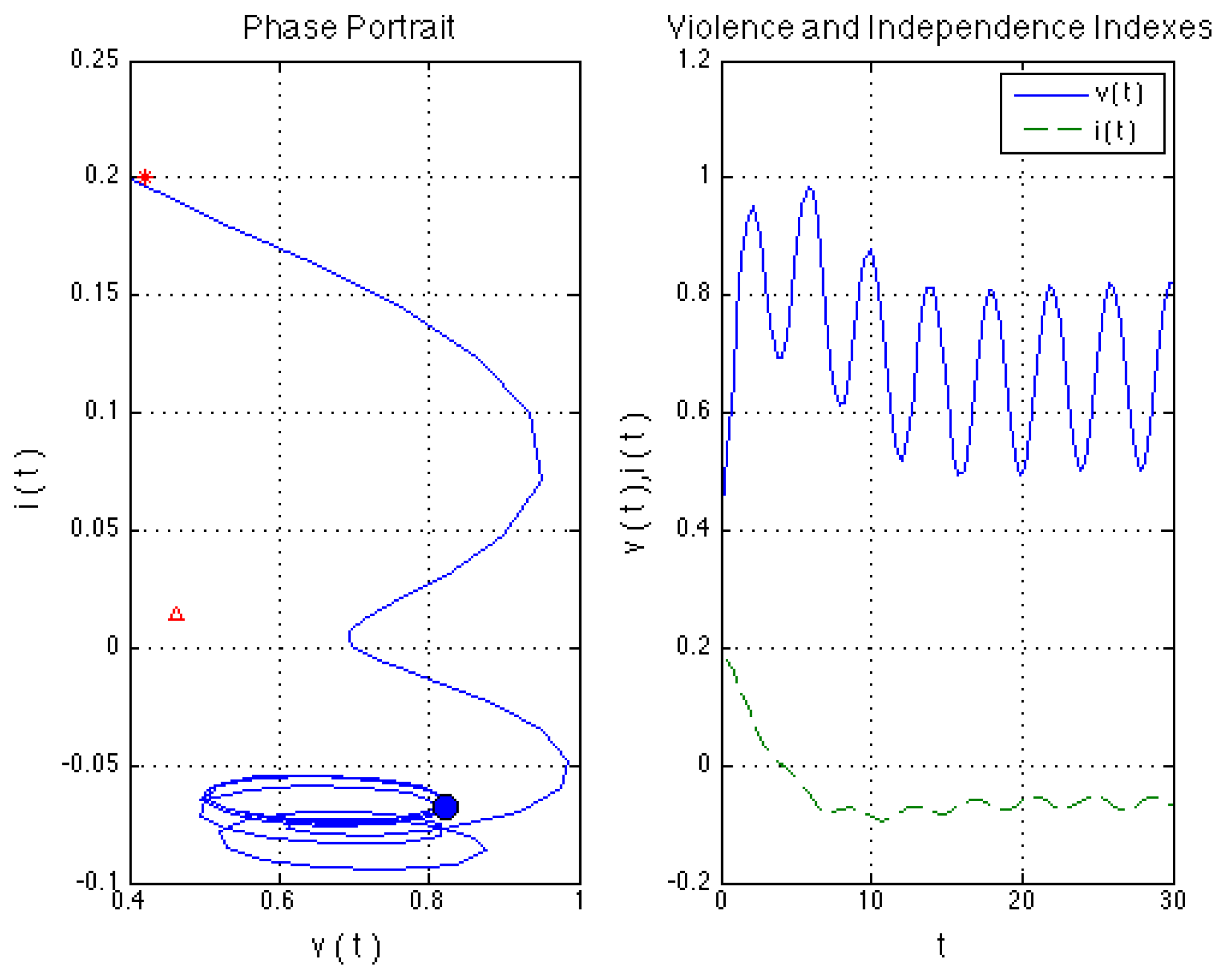
In this section, we present a classical and numerical analysis of Model (2). In order to accomplish this, we first analyze the model when there is not alcohol consumption. Later, we numerically analyze the complete model by considering alcoholism events.

Let us first assume that the function $h\left(t\right)\equiv 0$ because we are considering that the man does not consume alcohol periodically. This leads to an autonomous model. Thus, we start by determining the equilibrium points of the system (2) by making the derivatives equal to zero $\frac{dv}{dt}=0,\frac{di}{dt}=0$, and we solve for the model variables,

$$v^{*}=\frac{{\delta }_1{\delta }_2\tilde{v}+{\delta }_2{k}_1(1-{\rho }_1)({\beta }_1/\gamma )\tilde{i}}{{\delta }_1{\delta }_2-k_1{k}_2(1-{\rho }_1)(1-{\rho }_2)({\beta }_1/\gamma )\mu },i^{*}=\frac{{\delta }_1{\delta }_2\tilde{i}+{\delta }_1{k}_2(1-{\rho }_2)\mu \tilde{v}}{{\delta }_1{\delta }_2-k_1{k}_2(1-{\rho }_1)(1-{\rho }_2)({\beta }_1/\gamma )\mu }.$$

A simple inspection of $v^{*}$ and $i^{*}$ shows us that when $k_1=k_2=0$, we trivially recover the non-influenced steady state. It is more important to note that the equilibrium point of system (2) is now a linear combination of steady states $\tilde{v}$ and $\tilde{i}$. Observe that the denominator is the same for $v^{*}$ and $i^{*}$, and that it is a difference between the terms ${\delta }_1{\delta }_2$ and $k_1{k}_2(1-{\rho }_1)(1-{\rho }_2)({\beta }_1/\gamma )\mu$. The first one of these two expressions is in terms of rate of returning to the non-influenced steady states while the second depends on important factors for both of the intimate partners. Now, we determine the stability of the equilibrium point. For this, we compute the characteristic equation ${\lambda }^2-\tau \lambda +\Delta =0$ associated with the system. The roots of this equation are the eigenvalues of the coefficient matrix of the system and are given by, ${\lambda }_1=\frac{1}{2}\tau +\frac{1}{2}\sqrt{{\tau }^2-4\Delta }$ y ${\lambda }_2=\frac{1}{2}\tau -\frac{1}{2}\sqrt{{\tau }^2-4\Delta }.$ where $\tau =-{\delta }_1-{\delta }_2$ and $\Delta ={\delta }_1{\delta }_2-k_1{k}_2(1-{\rho }_1)(1-{\rho }_2)({\beta }_1/\gamma )\mu .$ Let us recall, that an equilibrium point is asymptotically stable if ${\tau }^2-4\Delta \ge 0$ and $\Delta \ge 0$ or ${\tau }^2-4\Delta <0$. In the case of ${\tau }^2-4\Delta >0$ and $\Delta <0$, we have that the equilibrium point is unstable. Let us discuss how these conditions apply to our model.

• Case 1. If ${\tau }^2-4\Delta <0,$ we have that ${({\delta }_1-{\delta }_2)}^2<-4k_1{k}_2(1-{\rho }_1)(1-{\rho }_2)({\beta }_1/\gamma )\mu$, then the equilibrium point $(v^{*},i^{*})$ is asymptotically stable, but the solutions are oscillating. A necessary condition is that $\mu <0$ which means that external factors make the woman’s independence index decrease. This may be caused by family or social pressure on the woman, or by her beliefs that lead her to a highly dependent state. In these circumstances, the IPV for this couple tends to the stable steady state which indicates woman submission and a constant level of IPV. It is important to remark that the left-hand side of the inequality is the difference between ${\delta }_1$ and ${\delta }_2$. Then, we can have this case when the inertia coefficients are very similar or equal, and there is social pressure on the woman. Another way in which this condition may hold corresponds to a high social pressure, low self-regulatory conditions, high acceptance of machismo or very low man’s self-esteem.
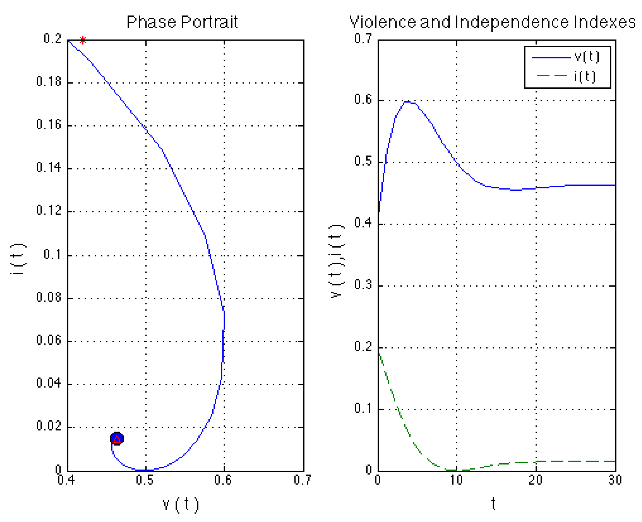
• Case 2. If ${\tau }^2-4\Delta \ge 0$ and $\Delta \ge 0$, or equivalently ${({\delta }_1-{\delta }_2)}^2\ge -4k_1{k}_2(1-{\rho }_1)(1-{\rho }_2)({\beta }_1/\gamma )\mu \ge -4{\delta }_1{\delta }_2$, then the equilibrium point is asymptotically stable and the solutions are not oscillatory. Notice that $\mu$ could be positive or negative. For this case, we can find a lot of possible parameter combinations which could lead us to this situation where the intimate partner interaction stabilizes rapidly. That means that the man’s violence and the woman’s independence indexes reach a stationary level and remain there for a long time. Observe that in this case, the inertias for both of the members of the couple could be similar or different, one from each other. However, independently of this, the level of IPV will be high when there exists high acceptance of machismo, low self-esteem or low self-regulation for the man. Otherwise, the model predicts a moderated level of IPV. Another fact is that depending on the $\mu$ value, the level of the woman’s independence will stabilize on a level of independence or dependency.
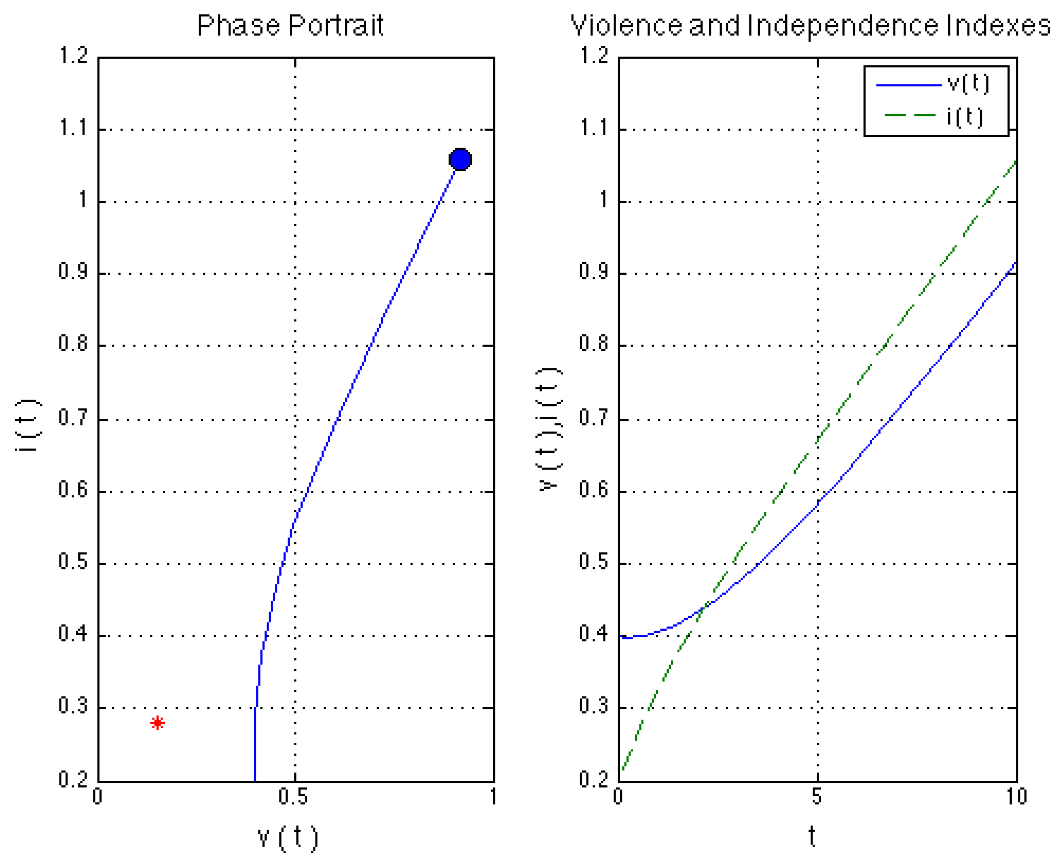
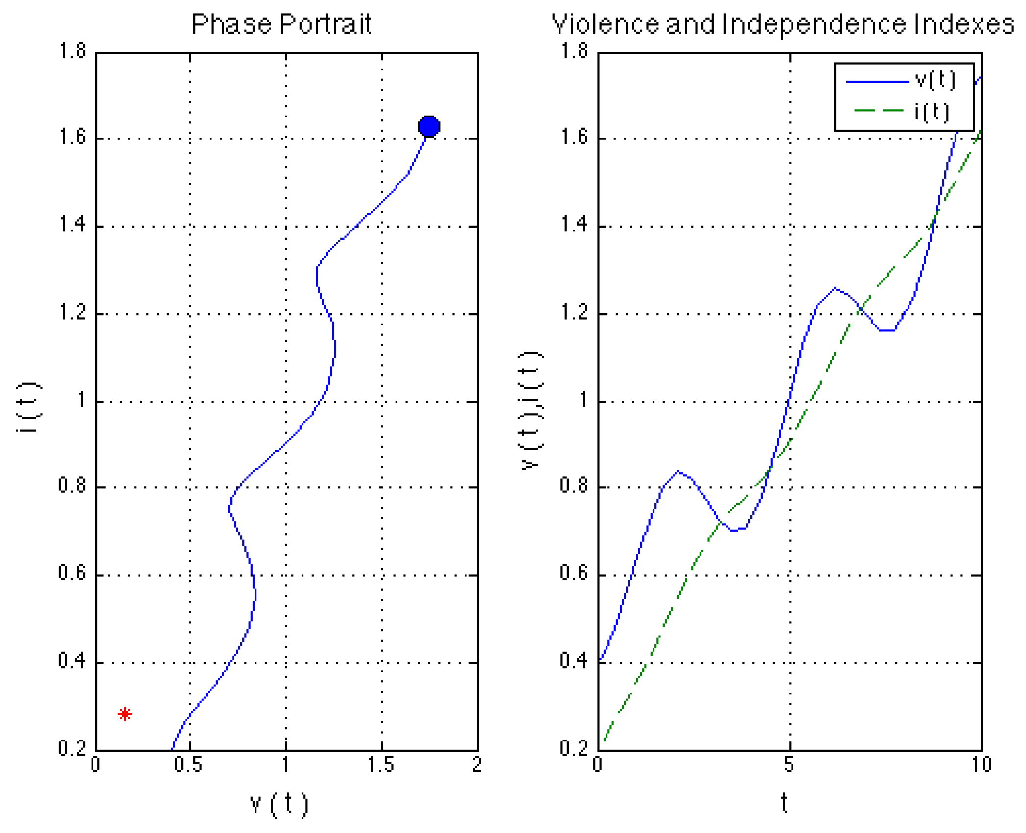
• Case 3. If ${\tau }^2-4\Delta >0$ and $\Delta <0$ or equivalently, ${\delta }_1{\delta }_2<k_1{k}_2(1-{\rho }_1)(1-{\rho }_2)({\beta }_1/\gamma )\mu$, then the equilibrium point is unstable and it is necessary that $\mu >0$ for the condition holds. Notice that the condition $\mu >0$ means that external factors are leading to an increment in the woman’s independence index. In particular, this could be achieved through empowerment programs for the woman. Then, our model reproduces the reported fact that this type of programs can lead to break the IPV cycle. But, it is important to remark that other situations must also occur. For example, if the coefficients ${\delta }_1$ and ${\delta }_2$ are relatively high, the coefficients ${\rho }_1$ and ${\rho }_2$ have to be close to zero, and ${\beta }_1$ high, or $\gamma$ small. In any case, we will have a steep climb on the IPV or the woman’s independence.

Let us recall that in the performed analysis we are considering no alcohol consumption. This will be addressed numerically in the next section.

4. Numerical Simulations

Now, we present simulations for the solutions of our model for different scenarios without and with man’s alcohol consumption. Let us say that the simulations where obtained using synthetic data for the parameters because we have no found any reported case where all parameters of the our model have been determined for a particular couple. However, we can define different parameter sets that corresponds to different situations or scenarios.

4.1. Model without Alcohol Consumption

In this subsection, we present different scenarios and its simulations of Model (2) for cases without man’s alcohol consumption. Before starting the discussion, let us explain the structure used in the figures. In each figure we can observe two graphs as well as the full set of parameters. The left-hand graphs are the phase portrait where only the indexes are shown. Also, we have marked with a star (∗) the non-influenced steady state point and with a triangle the influenced equilibrium point. For the right-hand side graphs, we have pictured the solutions as functions of time, $v\left(t\right)$ and $i\left(t\right)$ with time t in weeks. The choice of the time units is with the aim to compare the solutions with the alcohol consumption case, which is reported in weeks.

Scenario 1 Couple with a profile of moderated IPV. In this case, we consider a moderated violent man and a non-independent woman. We are assuming that both of the members of the couple have observed violence during their childhood, and they accept machismo as a lifestyle. This determines the non-influenced steady state. The rest of the parameters are such that the man’s self-esteem is medium as well as the self-regulatory level. With respect to the woman, its self-regulatory level is a medium level, and she is experiencing social pressure to continue in the relationship. Let us recall that for this case $h\left(t\right)=0$ because the man does not consume alcohol regularly. In Figure 2, we can observe that the solutions stabilize after an oscillatory behavior which corresponds to case 1, previously discussed. Also, that under these conditions the man’s violence index increases while the woman’s independence index reduces when it is compared with non-influenced steady state. This reduction usually is caused by a decrease in the woman’s self-esteem which could be explained as a consequence of the woman suffering IPV. On the other hand, let us remark that the maximum value of the violence index is $0.6$. If this value is extrapolated to the original scale, it corresponds to aggressions described as shaking and pulling to mistreat to the woman. For the level at which the violence index stabilize, we can say a daily man’s behavior corresponds to violent acts such as rough touching or destruction of personal belongings.

Scenario 2 Couple with a profile of moderated IPV and empowered woman. For this case, the parameters were set with values similar to the values of Scenario 1. Both of the members of the couple have observed a slightly medium level violence during their childhood, and they have a medium acceptance level of machismo. The man’s self-esteem is medium while that his self-regulatory parameter is lesser than the corresponding woman’s parameter value. The main change is that the woman empowerment is high as a consequence of being involved in empowerment programs. In Figure 3, we can observe that the solutions for both of the indexes increase rapidly. This is because the man responds violently to the increment in the woman’s independence. Let us recall that the man’s self-esteem is related to the man’s need to control the woman. For this case, violence reaches values so high that they escape of any real situation of IPV. Then, we can interpret this situation as a scenario where the woman faces severe violence perpetration (eventually the woman’s death when the violence index exceeds one). A more optimistic interpretation is that the relationship breaks because the woman’s independence increases faster than the IPV. It is important to remark that when the machismo acceptance or the man’s self-esteem is higher, the IPV grows even faster than the woman’s independence. Notice that influenced steady state cannot be reached by the solutions because it is non-stable.

4.2. Model with Alcohol Consumption

Now, we numerically analyze the model including the term that models the effect of alcoholism in the couple.

Scenario 3 Couple with a moderated profile of IPV and man’s alcohol consumption. In this case, we take the same parameter set of Scenario 1 and include the effect of the periodic alcohol consumption by the man ($h\left(t\right)\ne 0$), i.e., we are considering $\rho =0.25,\omega =\pi /2,\eta =0.35.$ In Figure 4, we can observe that the model with man’s periodic alcohol consumption follows the qualitative model behavior without alcohol consumption. In this case, the violence index increases and the independence index decreases, but the solution oscillates. Let us observe that, there is a time interval where the oscillations are changing in amplitude (transient behavior) to finally reach a periodic solution. Note the that maximum value of the violence index almost reach one, which corresponds to assassination attempt according to the IPN scale. Finally, the solution for $v\left(t\right)$ oscillates in an approximate range of $[0.5,0.8]$. When these values are interpreted according to IPV scale, they correspond to psychological and physical violent acts ranging from controlling the woman action, destroying personal belongings and death threats among others. We also note that there is the displacement of the steady state point, when it is compared with the case without alcohol consumption. This means that the man’s violence index and the woman’s dependency index increases, confirming that alcohol worsens the IPV perpetration. This agrees with the behavior reported one by the literature [2].

Scenario 4 Couple with a profile of empowered woman and man’s alcohol consumption. In this case, we take the parameter set of Scenario 2 and include the effect of the periodic alcohol consumption by the man ($h\left(t\right)\ne 0$), i.e., we add the parameters values $\rho =0.15,\omega =\pi /2,\eta =0.35.$ The results of this simulation are an oscillating increment in both of the indexes which is the same qualitative behavior found in the scenario 2, but with oscillations. See Figure 5. This even occurs more rapidly than in the case with a non-alcoholic man showing the emphasizing effect of periodic alcohol consumption.

Certainly, these all cases are undesirable and intervention strategies to avoid these situations are a must and will be discussed in the next section.

5. Discussion of the Model and Its Application

We have constructed a mathematical model based on measures of the human behavioral traits for the IPV dynamics in a romantic couple. Based on this model, it is very important to analyze possible applications. Also as a next step, we may ask about possible intervention strategies to reduce or to avoid violence. In order to do this, it is important to remark that our model reproduces a small number of reported situations of IPV which are boosted by alcoholism, considering only two variables. Notice, that despite it is very restrictive with respect to the IPV dynamics found in a romantic relationship, we can draw some interesting conclusions.

According to our model, there are two key parameters to change the IPV dynamics in a couple. The first one is the parameter ${\rho }_1$, which measures the self-regulatory factor of the IPV perpetrator. Certainly, the reason for introducing this factor is supported by the reported results in [16]. Especially by the fact that it can be used as an IPV predictor. In such a work, the authors argue that violent man impulses do not necessarily end in violent behavior. Moreover, this parameter value or human behavioral trait can be increased by providing the violence perpetrator with techniques to refrain from violent acts. Then, a possible intervention strategy could be to encourage this type of training. However, let us analyze the limit case ${\rho }_1=1$, recall that this parameter is normalized. Our model implies that woman independence does not contribute to increasing the violence in the couple. Then, the model suggests that violent behavior would tend to the non-influenced steady state which is not a zero violence state. Therefore, it is not enough to focus on the education of the perpetrator, but on the factors defining his intrinsic level of violence such as therapies to reduce the trauma caused by the violence watched in childhood. Additionally, educational programs to change man’s mind with respect to the machismo are needed.

Another possible strategy of intervention can be understood in terms of the empowering coefficient, $\mu$. By allowing it to take positive or negative values gives the opportunity to change the model dynamics. As a first scenario, with negative $\mu$, there are factors encouraging the woman to remain married, despite the level of violence that the woman is experiencing. Certainly, this simulates a cruel reality that must be avoided. As a first stage to achieve this, the woman must be enrolled in empowerment programs, ie. setting $\mu$ positive as a first step to break the violence cycle. violence caused by man’s need for control. One may suggest stressing the level of empowerment programs, but according to the model it will lead to increase the IPV. The suggested solution to escape IPV is to set conditions that ensure a more rapidly increment in the independence index with respect to violence increment. This is a consequence of the linearity of the model and points out the need to provide a more balanced model. Such improved model should reproduce more mild IPV scenarios. Also, it would be important to determine conditions where the violence can decrease while the woman independence increase. After that, it would follow the addition of modeling terms for the intervention strategies such as the couple therapy and public policy strategies. Both of them, with a short term impact in the reduction of the IPV problem.

6. Conclusions

In this work, we developed a model for the IPV perpetration in a romantic couple in terms of a system of linear differential equations. This model describes the cycle of violence in one couple by considering important causal and motivational factors. Among those factors, we consider that the most relevant is the inclusion of the need to control woman, the self-regulatory coefficients and the external factors for the woman. From our point of view, our contribution is the identification of important factors that trigger IPV and the corresponding use in setting a first differential equation model. Despite the simplicity of our model, it allowed us to reproduce different IPV scenarios and identify possible intervention strategies. In future work, we would like to explore the inclusion in the model of more realistic assumptions such as a variable self-regulatory coefficients, the inclusion of nonlinear terms to describe interactions. In particular those related with intervention strategies In this way, the model will reproduce more complex IPV scenarios and provide more targeted actions to reduce this social problem.

References

1. WHO Multi-Country Study on Women’s Health and Domestic Violence against Women: Summary Report of Initial Results on Prevalence, Health Outcomes and Women’s Responses. Available online: https://www.who.int/reproductivehealth/publications/violence/24159358X/en/ (accessed on 1 March 2019).
2. INEGI. Encuesta Nacional Sobre la Dinámica de las Relaciones en los Hogares. 2003. Available online: semujer.zacatecas.gob.mx/pdf/libros/Encuesta%20nacional%20sobre%20la%20dinamica%20de%20las%20relaciones%20en%20los%20hogares%202003%20ENDIREH.pdf (accessed on 1 March 2019).
3. Caprioli, M.; Hudson, V.M.; McDermott, R.; Ballif-Spanvill, B.; Emmett, C.F.; Stearmer, S.M. The Womanstats Project Database: Advancing an Empirical Research Agenda. J. Peace Res. 2009, 46, 839–851. [Google Scholar] [CrossRef]
4. Programme, U.N.D.; Malik, K. Human Development Report 2014: Sustaining Human Progress-Reducing Vulnerabilities and Building Resilience. Available online: http://hdr.undp.org/en/content/human-development-report-2014 (accessed on 1 March 2019).
5. Wiley, S.A.; Levy, M.Z.; Branas, C.C. The impact of violence interruption on the diffusion of violence: A mathematical modeling approach. In Advances in the Mathematical Sciences; Springer: Berlin, Germany, 2016; pp. 225–249. [Google Scholar]
6. Bourne, D.A. Mathematical Modeling of Pharmacokinetic Data; Routledge: Abingdon, UK, 2018. [Google Scholar]
7. DeAngelis, D.L. Individual-Based Models and Approaches in Ecology: Populations, Communities and Ecosystems; CRC Press: Boca Raton, FL, USA, 2018. [Google Scholar]
8. Sánchez, J.E.H.; Falconi, R.G. Instrumento para Medir el Empoderamiento de la Mujer; Universidad Juárez Autónoma de Tabasco: Villahermosa, Mexico, 2008. [Google Scholar]
9. Poza, E.; Jódar, L.; Barreda, S. Mathematical modeling of hidden intimate partner violence in Spain: A quantitative and qualitative approach. Abstr. Appl. Anal. 2016, 2016, 1–8. [Google Scholar] [CrossRef]
10. Gottman, J.; Swanson, C.; Murray, J. The mathematics of marital conflict: Dynamic mathematical nonlinear modeling of newlywed marital interaction. J. Fam. Psychol. 1999, 13, 3. [Google Scholar] [CrossRef]
11. Gottman, J.M. The Mathematics of Marriage: Dynamic Nonlinear Models; MIT Press: Cambridge, MA, USA, 2005. [Google Scholar]
12. Walker, L.E. The Battered Woman; Harper & Row: New York, NY, USA, 1980. [Google Scholar]
13. Corsi, J.; Dohmen, M.L.; Sotes, M.A. Violencia Masculina en la Pareja: Una Aproximación al Dignóstico y A los Modelos de Intervención; Paidos Argentina: Buenos Aires, Argentina, 1995. [Google Scholar]
14. Stith, S.M.; Farley, S.C. A predictive model of male spousal violence. J. Fam. Violence 1993, 8, 183–201. [Google Scholar] [CrossRef]
15. Kim, J.C.; Watts, C.H.; Hargreaves, J.R.; Ndhlovu, L.X.; Phetla, G.; Morison, L.A.; Busza, J.; Porter, J.D.; Pronyk, P. Understanding the impact of a microfinance-based intervention on women’s empowerment and the reduction of intimate partner violence in South Africa. Am. J. Public Health 2007, 97, 1794–1802. [Google Scholar] [CrossRef] [PubMed]
16. Finkel, E.J.; DeWall, C.N.; Slotter, E.B.; Oaten, M.; Foshee, V.A. Self-regulatory failure and intimate partner violence perpetration. J. Personal. Soc. Psychol. 2009, 97, 483. [Google Scholar] [CrossRef] [PubMed]
17. Olaiz, G.; Rico, B.; Del Río, A. Encuesta Nacional sobre Violencia contra las Mujeres 2003; Instituto Nacional de Salud Pública: Cuernavaca Mor., Mexico, 2004. [Google Scholar]
18. Carson, A.T.; Baker, R.C. Psychological correlates of codependency in women. Int. J. Addict. 1994, 29, 395–407. [Google Scholar] [CrossRef] [PubMed]
19. Thompsn, M.P.; Basile, K.C.; Hertz, M.F.; Sitterle, D. Measuring Intimate Partner Violence Victimization and Perpetration: A Compendium of Assessment Tools; National Center for Injury Prevention and Control: Atlanta, GA, USA, 2006.
20. Valdez-Santiago, R.; Híjar-Medina, M.C.; Salgado de Snyder, V.N.; Rivera-Rivera, L.; Avila-Burgos, L.; Rojas, R. Escala de violencia e índice de severidad: una propuesta metodológica para medir la violencia de pareja en mujeres mexicanas. Salud Pública de México 2006, 48, s221–s231. [Google Scholar] [CrossRef] [PubMed]
21. Tronco Rosas, M.A. No sólo Ciencia y Tecnología. Ahora, el IPN a la Vanguardia en Perspectiva de género. El Programa Institucional de Gestión con Perspectiva de Género. Available online: http://www.genero.ipn.mx/Conocenos/Documents/MemoriaPIGPG.pdf (accessed on 1 March 2019).
22. Garcia, D.; Weber, I.; Garimella, V.R.K. Gender Asymmetries in Reality and Fiction: The Bechdel Test of Social Media. In Proceedings of the 8th International AAAI Conference on Weblogs and Social Media, Ann Arbor, MI, USA, 1–4 June 2014; pp. 131–140. [Google Scholar]
23. Gil-González, D.; Vives-Cases, C.; Ruiz, M.T.; Carrasco-Portino, M.; Álvarez-Dardet, C. Childhood experiences of violence in perpetrators as a risk factor of intimate partner violence: A systematic review. J. Public Health 2007, 30, 14–22. [Google Scholar] [CrossRef] [PubMed]
24. Arciniega, G.M.; Anderson, T.C.; Tovar-Blank, Z.G.; Tracey, T.J. Toward a Fuller Conception of Machismo: Development of a Traditional Machismo and Caballerismo Scale. J. Couns. Psychol. 2008, 55, 19–33. [Google Scholar] [CrossRef]
25. Bendezú, A. Los estereotipos de género y el riesgo del embarazo adolescente. Ph.D. Thesis, UNAM, México City, México, 1998. [Google Scholar]
26. Robins, R.W.; Hendin, H.M.; Trzesniewski, K.H. Measuring Global Self-Esteem: Construct Validation of a Single-Item Measure and the Rosenberg Self-Esteem Scale. Personal. Soc. Psychol. Bull. 2001, 27, 151–161. [Google Scholar] [CrossRef]
27. Sinclair, V.G.; Wallston, K.A. The Development and Psychometric Evaluation of the Brief Resilient Coping Scale. Assessment 2004, 11, 94–101. [Google Scholar] [CrossRef] [PubMed]
28. Calleja, N. Escalas Psicosociales en México. Available online: http://www.psicologia.unam.mx/documentos/pdf/repositorio/InventarioEscalasPsicosocialesNaziraCalleja.pdf (accessed on 1 March 2019).
Figure 1. Diagram of model (2) showing the variables and their interaction terms.
Mca 24 00029 g001
Figure 2. Violent man without alcohol consumption and submissive woman. α 1 = 0.7 , α 2 = 0.6 , β 1 = 0.6 , β 2 = 0.5 , γ = 0.5 , δ 1 = 0.2 , δ 2 = 0.25 , ρ 1 = 0.5 , ρ 2 = 0.5 , μ = 0.2 , ( v ( 0 ) , i ( 0 ) ) = ( 0.4 , 0.2 ) .
Mca 24 00029 g002
Figure 3. Violent man without alcohol consumption, empowerment woman. α 1 = 0.5 , α 2 = 0.6 , β 1 = 0.3 , β 2 = 0.3 , γ = 0.6 , δ 1 = 0.25 , δ 2 = 0.25 , ρ 1 = 0.5 , ρ 2 = 0.5 , μ = 0.6 , ( v ( 0 ) , i ( 0 ) ) = ( 0.4 , 0.2 ) .
Mca 24 00029 g003
Figure 4. Violent man with alcohol consumption, non-independent woman. α 1 = 0.7 , α 2 = 0.6 , β 1 = 0.6 , β 2 = 0.5 , γ = 0.5 , δ 1 = 0.2 , δ 2 = 0.25 , ρ 1 = 0.5 , ρ 2 = 0.5 , μ = 0.2 , ρ = 0.25 , ω = π / 2 , η = 0.35 .
Mca 24 00029 g004
Figure 5. Violent man with alcohol consumption, empowered woman. α 1 = 0.5 , α 2 = 0.6 , β 1 = 0.3 , β 2 = 0.3 , γ = 0.6 , δ 1 = 0.25 , δ 2 = 0.25 , ρ 1 = 0.5 , ρ 2 = 0.5 , μ = 0.6 , ρ = 0.25 , ω = π / 2 , η = 0.35 .
Mca 24 00029 g005