Effect of Temperature on Diluate Water in Batch Electrodialysis Reversal

Abstract

A high percentage of the agricultural wells in the state of Sonora are overexploited, thus generating a significant degree of saline intrusion and abandonment by nearby communities. In this paper, the effect of temperature on the final concentration of diluted water was evaluated with variations in voltage and input concentration in a batch electrodialysis reversal (EDR) process in order to find the optimal operating conditions, with an emphasis on reducing the energy consumption and cost of desalinated water. Thirty-six samples were prepared: eighteen samples of 2000 mg/L total dissolved solids (TDS) and eighteen samples of 5000 mg/L TDS; brackish well water of 639 mg/L TDS and synthetic salt were mixed to obtain these concentrations. Three different temperatures (25, 30, and 35 °C) and two different voltages (10 and 20 V) were tested for each sample after evaluating the limiting current density. The best salt removal occurred in the 20 V sets, with 18.34% higher removal for the 2000 mg/L TDS experiments and 25.05% for the 5000 mg/L experiments (average between the 25 to 35 °C tests). The temperature positively affected the EDR, especially in the experiments at 10 V, where increasing by 10 °C increased the efficiency by 10.83% and 24.69% for 2000 and 5000 mg/L TDS, respectively. The energy consumption was lower with increasing temperature (35 °C), as it decreased by 1.405% and 1.613% for the 2000 and 5000 mg/L TDS concentrations, respectively (average between the 10 and 20 V tests), thus decreasing the cost per m³ of water.

1. Introduction

On Earth, water is the most valuable resource for the development of living beings due to its importance in cellular metabolism and its use in many human activities (household, agriculture, and industry). Unlike other natural resources, water is renewed by introducing approximately 505,000 km³ each year through the hydrological cycle [1]. However, 2.1 billion people in the world do not have access to safe drinking water as a result of overexploitation, contamination, and poor distribution [2].

In the state of Sonora, located in northwestern Mexico, 90% of the region presents desert and arid conditions, with temperatures above 40 °C. It has a normal average precipitation of 297 and 483 mm in the north and south, respectively [3], which is below the national average. On the other hand, the state’s renewable water per capita is 2385 m³/year/inhabitant [3], which represents a volume that is 9% lower than the national per capita value, despite being the second-largest state in Mexico.

Water availability problems in the region’s aquifers are due to overexploitation and saline intrusion, thus causing a high concentration of salts in their wells [4]. The brackish water (BW) in them, when used for irrigation, impairs soil properties and crop vegetative development [5]. In addition, in 30 wells of the Hermosillo Coast aquifer, a study by Monreal et al. [6] detected that seawater intrusion has persisted since the 1960s.

Given the above problems, the opportunity to implement water desalination systems has arisen. These are capable of reducing the total dissolved solids (TDS) from a saline solution and operate from a chemical, electrical, or thermal potential [7]. Desalination processes can be classified in various ways [8,9,10]; however, thermal and membrane systems are the most commonly employed for brackish water and seawater.

Among membrane systems, electrodialysis (ED) is a technology that uses ion exchange membranes and an applied electric current to separate salts from an aqueous medium. The feed stream crosses an array of cells (its elementary unit), consisting of an anion exchange membrane (AEM) and cation exchange membrane (CEM), which selectively attract the ions in the solution and generate alternating compartments where the salts are simultaneously concentrated and reduced. The membranes are mostly composed of a high density of ionic groups, which allows the selective transport of ions across it depending on their charge. Counter-ions (of the opposite charge) are allowed to pass through, while co-ions (same charge) are prevented from passing through due to Donnan repulsion [11] (Figure 1).

Electrodialysis reversal (EDR) works with the same mechanism as electrodialysis, except that the polarity of the electrodes is periodically reversed (approximately 3 to 4 times per hour) and, by means of automatic valves, the outputs of the concentrated solution and the dilute solution are exchanged. In this way, the ions are transferred in opposite directions, which hinders the formation of fouling and allows the membranes to be washed [13].

Electrodialysis is mainly used in low- to medium-scale plants with capacities of less than 100 m³/d to slightly more than 20,000 m³/d. The success of electrodialysis is observed to a greater extent when water with a total salt concentration of less than 10,000 mg/L is handled. On the other hand, reverse osmosis systems are preferred for feed sources with salinities close to those of seawater or brine. In this context, ED and EDR are attractive due to their cost-effectiveness when treating brackish sources [11,14].

The operation in these systems is carried out on a continuous basis when large-scale and stable water production is needed; however, such installations require a large number of membranes and, therefore, suffer from large pressure drops and high energy demand [15]. In regions of Sonora where water availability is scare, batch operation is ideal because it allows desalination of brackish water to a potable level in minutes; also, the production cost is lower compared to that of reverse osmosis [16,17].

Transport in ion exchange membranes can be described as the combined effect of the diffusive flux generated by the concentration gradient in the boundary layer and the flux due to ion migration in the membrane. The transport phenomenon can be expressed mathematically by the Nernst–Planck equation [18]:

$$J_i=-D_i\frac{d{C}_i}{dz}-D_i\frac{z_i{C}_{i}F}{RT}\frac{dV}{dz}$$

(1)

where $i$ refers to a component of the solution, $D$ represents the diffusivity of the solution, $C$ is the concentration, $V$ is the electrical potential, $F$ is the Faraday number, $R$ is the gas constant, $T$ is the absolute temperature, $z$ is the charge number and $dz$ is a directional coordinate. It expresses how the mass flux over the membrane is enhanced as voltage increases, generating greater current densities and a performance improvement [12]. However, when a difference between the ion transport numbers on the membrane surface and inside the bulk flow is established, ions begin to be accumulated and depleted on the membrane sides of the concentrated and diluate compartments, respectively; this phenomenon is called concentration polarization. As a consequence, the ion concentration near the membrane approaches zero, and the current density is limited [19]. This generates a greater voltage drop, which increases energy consumption and causes water dissociation [20]. The limiting current density can be estimated by plotting the applied current over the membrane against the membrane potential. Two main regions can be identified on this curve: a proportional current–voltage variation (ohmic regime) and a plateau where the limiting current density begins [19].

Temperature plays an important role in ion transport, since the diffusivity of species $i$ ($D_i$) and ion mobility (${\nu }_i=D_i/RT$) have been found to be a function of temperature, and its effect expresses a greater influence on diffusive flux in contrast to ion migration flux [21]. Another positive consequence of increasing temperature is the decrease in the electrical resistance of membranes to ion passage [22].

In this paper, the physicochemical parameters of the outlet stream in a batch electrodialysis reversal of BW are experimentally evaluated by increasing the temperature in order to define an optimal operating range for the membranes. Two concentrations, two applied voltages, and three different temperatures in the feed stream were applied to construct a factorial arrangement. The imposed temperatures were selected without exceeding the limit supported by the membranes. The percentage of ions extracted is expected to improve with increasing voltage and temperature, and it was desired to know the extent to which this happens in a batch process. In addition, an economic evaluation of potable water production in terms of the energy costs of the overall process was carried out.

2. Materials and Methods

2.1. Study Area and Preparation of Feed Water

The experiment and brackish water collection were conducted at 28° 36′ 0′′ North, 111° 31′ 1′′ West in Ciudad Obregón, Sonora, Mexico, at the Marine Water Desalination Research Laboratory. A total of 36 BW samples were prepared at different concentrations: 18 samples at 2000 mg/L TDS and 18 samples at 5000 mg/L TDS. This was done by mixing some water from wells of the region (639 mg/L TDS) and a saline solution, which was prepared with synthetic salt and distilled water.

2.2. System CIP

To guarantee the reliability of the equipment, a counter-current chemical cleaning was performed to avoid contamination in the tests. First, the three tanks—diluate (T-1), concentrate (T-3), and electrode waste (T-2)—were washed with tap water (Figure 2). After draining the liquid, 1 L of distilled water was added to each tank, and the electrodialysis equipment was connected to a 110 V electric current. It was always necessary to check the valve arrangement, keeping valves 1, 2, and 3 open and valves 4–10 closed. Subsequently, the circulation pumps were turned on for 1 min to homogenize, and finally, the water was drained.

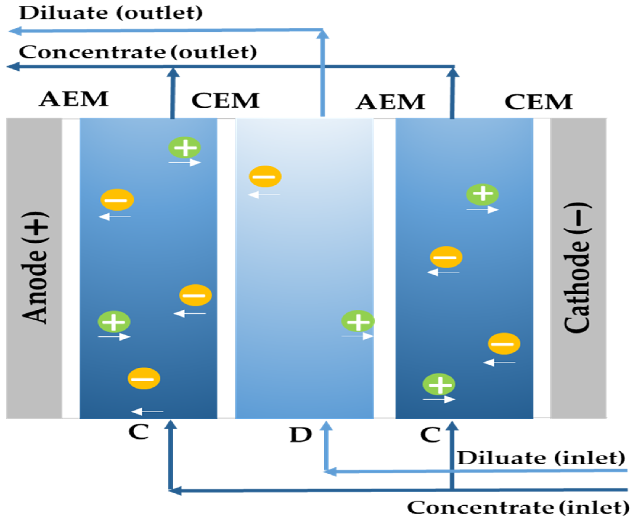
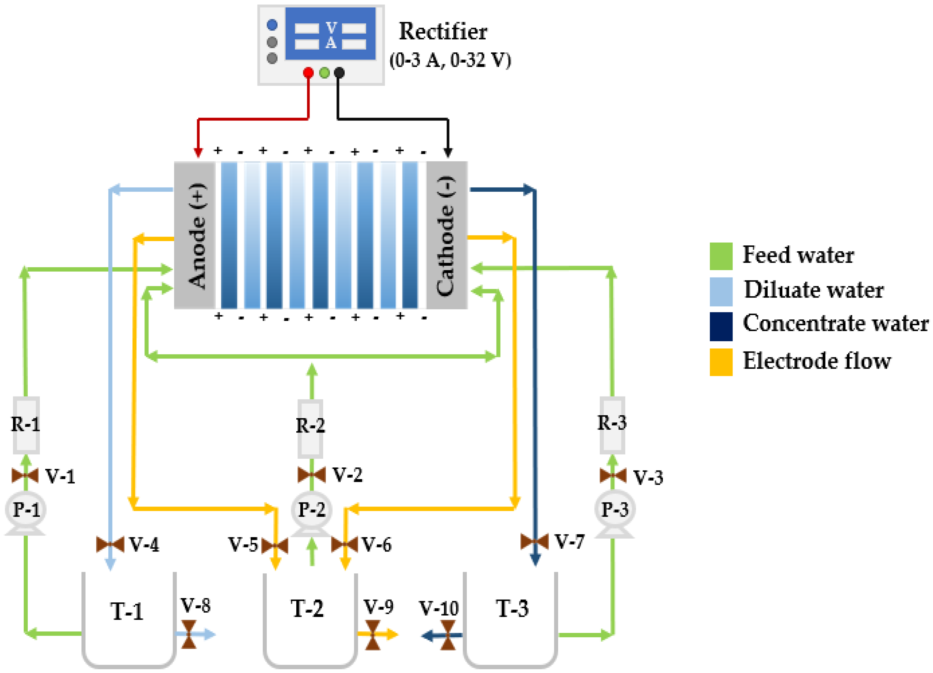
2.3. Description of the Electrodialysis Equipment

An ED/EDR system with a rate of 50 L/h was used to perform the BW desalination tests. The system had 5 CEMs and 5 AEMs from Asahi, three 0.1 HP centrifugal pumps, a 0.5-inch polyvinyl chloride (PVC) piping arrangement, 10 valves for flow circulation and sample collection, and three rotameters that were graduated at 20 L/min. The electrodes where the experimental voltage was applied, which divided the surfaces of the cationic and anionic membranes, were made of stainless steel 316 and platinized titanium, respectively (see Figure 2). A rectifier charge controller was connected to the electrodes by the red and black wire. The specific parameters of the rectifier are: nominal voltage: 220 V/110 V, max. current: 3 A, max. adjustable voltage: 32 V, Model 1672 BX-Precision. Lastly, the diluate, concentrate, and electrode waste tanks were 3 L (T-1, T-2, and T-3).

In

Table 1. Membrane design parameters.

Parameter	Value
Cell thickness (m)	0.0015
Cell height (m)	0.180
Cell width (m)	0.0925
Cell area (cm2)	166.5
Membrane thickness (m)	0.020
Membrane height (m)	0.180
Membrane width (m)	0.0925
Membrane area (cm2)	166.5

are shown the membrane design parameters.

2.4. Limiting Current Density Tests

Limiting current density (LCD) experiments were performed for each initial concentration (2000 and 5000 mg/L) with a feed stream of 50 L/h at 25 °C. Two current density (mA/cm²) vs. voltage (V) plots were obtained with the method described by [23]. Every minute, the voltage was increased, and the corresponding amperage was measured. The total measurement time was 64 min, and the voltage was varied from 0 to 30 V with 0.5 V increments. The graphs were the means of 3 repetitions.

2.5. Setup of EDR Experiments

A 3-factor factorial arrangement was designed for 12 different tests in triplicate. For this, three temperatures (25, 30, and 35 °C), two voltages (10 and 20 V), and two initial concentrations (2000 and 5000 mg/L) were used.

2.6. Operation of EDR Equipment

A total of 9 L of water was heated from an electric resistance (water heater), homogenized with a propeller agitator, and poured in the same proportion into the three tanks (3 L per tank). Subsequently, the three pumps were turned on to prepare the equipment, and the voltage was adjusted using the rectifier. Six samples were collected from the concentrate tank and six from the diluate tank at different times throughout the experiment, as shown in

Table 2. Sample collection interval.

Sample	Time (min)
1	4
2	7
3	10
4	13
5	16
6	19

. In order to maintain consistency with the measurements of the other tests, the experiment ended at 19 min. A wattmeter was used to record the energy consumed by the pump system and the rectifier during each experiment.

2.7. Process Control Parameters

The parameters used to control and monitor the evolution of the process were the percentage of ions extracted (%) and the conversion (%) [24]. The percentage of ions extracted (PIE) of the experiments was estimated as the ratio of the salts removed with respect to the salts initially contained:

$$\mathrm{PIE}=\frac{{\mathit{TDS}}_i-{\mathit{TDS}}_f}{{\mathit{TDS}}_i}\times 100$$

(2)

where ${\mathit{TDS}}_i$ and ${\mathit{TDS}}_f$ are the initial and final total dissolved solids concentration, respectively. The recovery percentage (R_%) was the volume fraction of water that was obtained as diluate; it was obtained through the following equation:

$$\mathrm{R}\%=\frac{Q_D}{Q_F}\times 100=\frac{Q_D}{Q_C+Q_D}\times 100$$

(3)

The typical recovery used in electrodialysis is around 85–90% [25]; however, in all experiments, a water conversion rate of 50% was maintained to avoid overloading the pumping system beyond its capacity.

3. Results and Discussion

3.1. Characteristics of Well Water

The characteristics of the well water sample from which the feed water was made are shown in

Table 3. Characteristics of well water.

Parameters	Value
Volume (L)	300 ± 0.2
TDS (mg/L)	638 ± 4.8
pH	8.19 ± 0.1
Electrical conductivity (mS/cm)	0.992 ± 0.007
Temperature (°C)	19.91 ± 1.3

.

3.2. Limiting Current Density Test Results

The results of the limiting current density profile are shown in Figure 3. It can be observed that the plateau for both the 2000 and 5000 mg/L samples appeared beyond 10 V at a current density of around 3 and 7 mA/cm², respectively. The limiting current density values in the ED/EDR process prior to a routine operation process allow one to know the maximum value of the electric current of the system in operation; thus undesired reactions, such as water dissociation, which causes a loss of current utilization, can be avoided [19,20]. In this regard, the nominal operating conditions for the 2000 and 5000 mg/L TDS samples were set to 10 and 20 V in order to see if the effects of temperature were maintained at applied potentials beyond 10 V in both concentrations.

3.3. Effect of Applied Voltage (10 and 20 V)

In the following section, the overall behavior of the TDS concentrations of the streams over time and the effects of the changes in voltage are explained by means of TDS plots of the diluate and concentrated streams for each experiment at a fixed temperature (Figure 4 and Figure 5). The orange and brown dotted curves correspond to the concentrated streams in the experiments at 10 and 20 V, respectively; moreover, the green and blue dotted curves correspond to the diluate streams in the experiments at 10 and 20 V, respectively. The results of the 12 tests performed are shown in

Table A1. Desalination results for the 2000 mg/L TDS sample at 25 °C.

Time (min)	10 V				20 V
	Diluate Water		Concentrated Water		Diluate Water		Concentrated Water
	EC (mS/cm)	TDS (mg/L)	EC (mS/cm)	TDS (mg/L)	EC (mS/cm)	TDS (mg/L)	EC (mS/cm)	TDS (mg/L)
0	3.14	2020.55	3.14	2020.55	3.15	2031.50	3.15	2028.60
4	2.63	1695.33	3.31	2128.42	2.03	1309.25	3.77	2426.16
7	2.30	1477.98	3.73	2404.37	1.51	974.37	4.41	2842.62
10	1.92	1234.87	3.96	2548.31	0.95	613.09	4.76	3066.94
13	1.51	970.19	4.31	2775.96	0.57	367.72	5.12	3298.57
16	1.18	757.67	4.78	3080.90	0.39	285.94	5.32	3426.72
19	0.92	589.26	5.15	3319.18	0.22	142.97	5.50	3541.36

,

Table A2. Desalination results for the 2000 mg/L TDS sample at 30 °C.

Time (min)	10 V				20 V
	Diluate Water		Concentrated Water		Diluate Water		Concentrated Water
	EC (mS/cm)	TDS (mg/L)	EC (mS/cm)	TDS (mg/L)	EC (mS/cm)	TDS (mg/L)	EC (mS/cm)	TDS (mg/L)
0	3.12	2009.28	3.12	2009.28	3.12	2010.25	3.11	2005.85
4	2.45	1575.87	3.29	2115.54	2.14	1374.94	3.58	2303.37
7	2.05	1317.62	3.65	2351.89	1.63	1046.50	4.32	2780.58
10	1.79	1150.51	4.06	2612.06	0.83	592.48	4.77	3071.45
13	1.53	878.09	4.35	2799.79	0.57	366.01	5.02	3232.45
16	1.04	667.83	4.59	2955.64	0.40	257.92	5.39	3469.44
19	0.85	545.15	4.77	3070.27	0.21	136.85	5.53	3564.11

,

Table A3. Desalination results for the 2000 mg/L TDS sample at 35 °C.

Time (min)	10 V				20 V
	Diluate Water		Concentrated Water		Diluate Water		Concentrated Water
	EC (mS/cm)	TDS (mg/L)	EC (mS/cm)	TDS (mg/L)	EC (mS/cm)	TDS (mg/L)	EC (mS/cm)	TDS (mg/L)
0	3.11	1999.62	3.11	1999.62	3.14	2023.13	3.14	2021.73
4	2.13	1374.62	3.48	2242.09	1.84	1181.74	3.66	2356.40
7	1.73	1115.73	3.96	2548.63	1.40	902.24	4.29	2763.40
10	1.35	869.40	4.27	2752.78	0.89	570.58	4.76	3066.94
13	0.88	565.75	4.59	2954.99	0.56	360.64	5.04	3244.90
16	0.68	435.67	4.82	3103.44	0.31	200.28	5.28	3398.39
19	0.57	366.44	5.06	3257.67	0.18	116.56	5.39	3468.37

,

Table A4. Desalination results for the 5000 mg/L TDS sample at 25 °C.

Time (min)	10 V				20 V
	Diluate Water		Concentrated Water		Diluate Water		Concentrated Water
	EC (mS/cm)	TDS (mg/L)	EC (mS/cm)	TDS (mg/L)	EC (mS/cm)	TDS (mg/L)	EC (mS/cm)	TDS (mg/L)
0	7.86	5064.63	7.86	5064.63	7.79	5015.15	7.79	5015.15
4	6.83	4397.45	7.93	5104.56	5.74	3697.20	8.24	5307.53
7	6.22	4008.69	8.48	5462.19	4.95	3185.22	9.56	6157.61
10	5.65	3641.18	8.94	5756.29	3.75	2415.64	10.53	6781.32
13	4.86	3126.83	9.46	6091.17	2.78	1788.39	11.41	7344.82
16	4.25	2738.29	9.86	6351.56	2.05	1319.23	12.10	7792.40
19	3.75	2414.14	10.33	6651.45	0.97	623.39	12.78	8230.32

,

Table A5. Desalination results for the 5000 mg/L TDS sample at 30 °C.

Time (min)	10 V				20 V
	Diluate Water		Concentrated Water		Diluate Water		Concentrated Water
	EC (mS/cm)	TDS (mg/L)	EC (mS/cm)	TDS (mg/L)	EC (mS/cm)	TDS (mg/L)	EC (mS/cm)	TDS (mg/L)
0	7.82	5038.44	7.82	5038.44	7.70	4958.16	7.69	4954.72
4	6.33	4073.51	8.39	5401.87	5.00	3218.39	8.84	5693.39
7	5.80	3733.05	9.16	5897.97	3.93	2528.99	10.33	6654.67
10	4.92	3168.05	9.90	6374.53	2.79	1799.66	11.38	7326.57
13	4.19	2700.51	10.61	6832.84	1.93	1241.63	12.25	7889.00
16	3.48	2240.48	11.15	7182.75	1.25	807.90	12.69	8174.51
19	2.93	1889.07	11.60	7468.25	0.81	520.35	13.14	8464.31

and

Table A6. Desalination results for the 5000 mg/L TDS sample at 35 °C.

Time (min)	10 V				20 V
	Diluate Water		Concentrated Water		Diluate Water		Concentrated Water
	EC (mS/cm)	TDS (mg/L)	EC (mS/cm)	TDS (mg/L)	EC (mS/cm)	TDS (mg/L)	EC (mS/cm)	TDS (mg/L)
0	7.81	5027.71	7.81	5029.00	7.80	5021.27	7.79	5015.90
4	6.28	4046.47	8.31	5348.42	4.92	3167.84	9.04	5823.48
7	5.36	3454.20	9.45	6087.95	3.16	2034.07	10.32	6643.50
10	4.33	2785.51	10.51	6766.29	2.29	1472.18	11.61	7474.69
13	3.39	2181.01	11.06	7124.79	1.62	1045.21	12.33	7938.37
16	2.65	1709.18	11.83	7616.59	1.14	733.19	12.93	8326.92
19	1.79	1155.55	12.42	7998.48	0.79	506.18	13.50	8696.15

in Appendix A.

In Figure 4 and Figure 5, for every diluate stream, the TDS concentration decreased over time, while the concentration of every concentrated stream increased as time marched on, as would be expected in an electrodialysis process. It can be seen that the 2000 mg/L feed water tests were able to reach concentrations below 590 and 150 mg/L when voltages of 10 and 20 V were applied, respectively. On the other hand, the 5000 mg/L tests achieved a diluate concentration between 2500 and 1000 mg/L at 10 V and below 630 mg/L at 20 V. In addition, the ratio between the diluate water concentration (D) of the 10 and 20 V tests (green and blue dotted curve) was estimated in order to visualize how much greater the concentrations in the 10 V tests were in comparison to those in the 20 V tests.

Table 4. Diluate stream concentration ratio between the 10 and 20 V tests.

Time (min)	D10V/D20V
	2000 mg/L			5000 mg/L
	25 °C	30 °C	35 °C	25 °C	30 °C	35 °C
0	1	1	1	1	1	1
4	1.2949	1.1461	1.1632	1.1894	1.2657	1.2774
7	1.5169	1.2591	1.2366	1.2585	1.4761	1.6982
10	2.0142	1.9419	1.5237	1.5073	1.7604	1.8921
13	2.6384	2.3991	1.5687	1.7484	2.1750	2.0867
16	2.6498	2.5893	2.1753	2.0757	2.7732	2.3312
19	4.1216	3.9836	3.1438	3.8726	3.6304	2.2829

shows these results for all measurement times in every test. The D_10V/D_20V value of minute 0 was established as 1, since the calculated ratios were due to the small differences in the initial concentrations among all samples.

In Table 4, it can be seen that, for all experiments, the D_10V/D_20V ratio increases as time progressed, which indicates that, for a given initial concentration and at a fixed temperature, the desalting process carried out in the 20 V tests was faster than that in the 10 V tests. This makes it clear that the larger imposed voltage removed a greater amount of salts by the end at 19 min. In addition, it can be seen that the D_10V/D_20V ratio of the 5000 mg/L tests was lower compared to that in the 2000 mg/L tests. The dependence on voltage can be described by Equation (1), which models the transport of ions in the membranes as a proportional function of the voltage. This explains how the electric field strength influences electromigration through membranes and demonstrates that in experiments in which a voltage of 20 V is applied, a higher removal of TDS will be achieved [26].

Table 5. Difference in the efficiency of experiments at 10 and 20 V.

Case	Arrangement	Ions Extracted (%) 10 V	Ions Extracted (%) 20 V	Difference (%)
1	2000 SDT-25 °C	70.84 ± 7.35	92.96 ± 2.38	22.13
2	2000 SDT-30 °C	72.87 ± 13.45	93.19 ± 3.68	20.32
3	2000 SDT-35 °C	81.67 ± 10.88	94.24 ± 0.11	12.56
4	5000 SDT-25 °C	52.33 ± 18.25	87.57 ± 1.33	35.24
5	5000 SDT-30 °C	62.51 ± 14.95	89.5 ± 1.25	27.01
6	5000 SDT-35 °C	77.02 ± 10.62	89.92 ± 4.28	12.90

presents the percentage of ions extracted (removal ratio) for every applied voltage in all cases and the increases between them. Is noteworthy that the increment in the removal efficiency was slightly larger when compared to its counterpart at the initial concentration, i.e., for case 1 there was a difference of 22.13% between the 10 and 20 V tests, while for case 4 there was a difference of 35.24%. Clearly, the main reason for this is due to the larger voltage imposed.

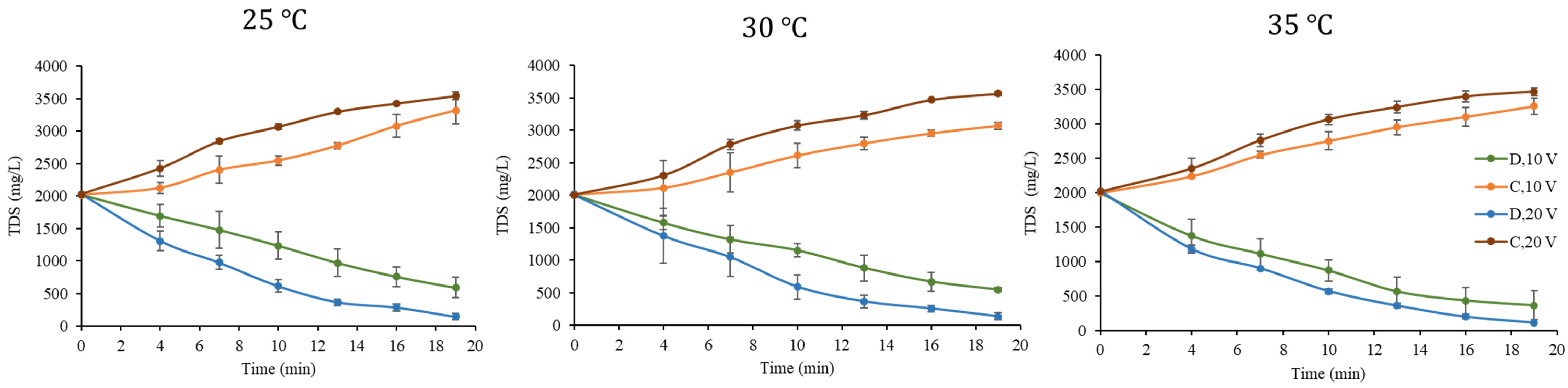
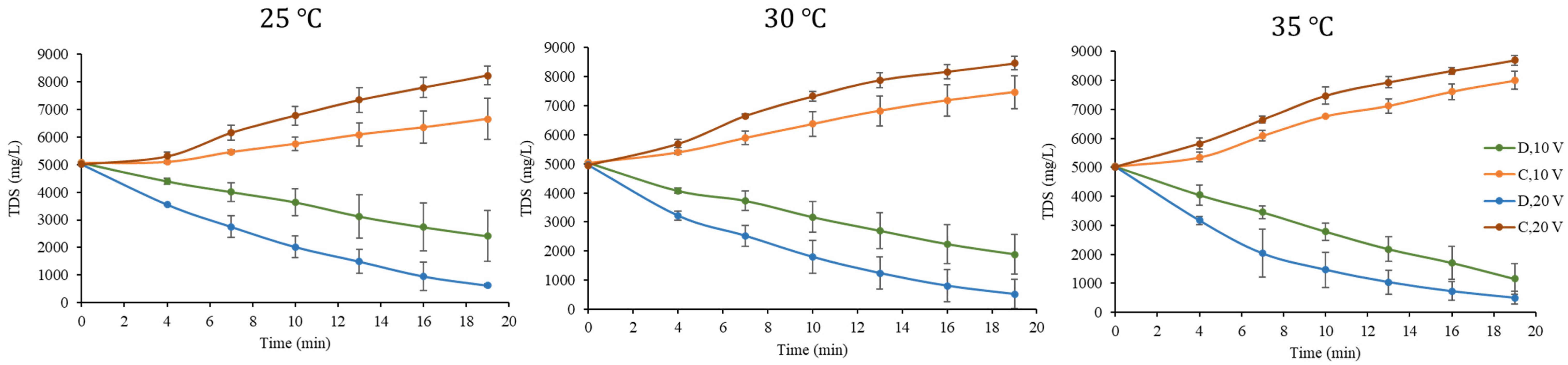
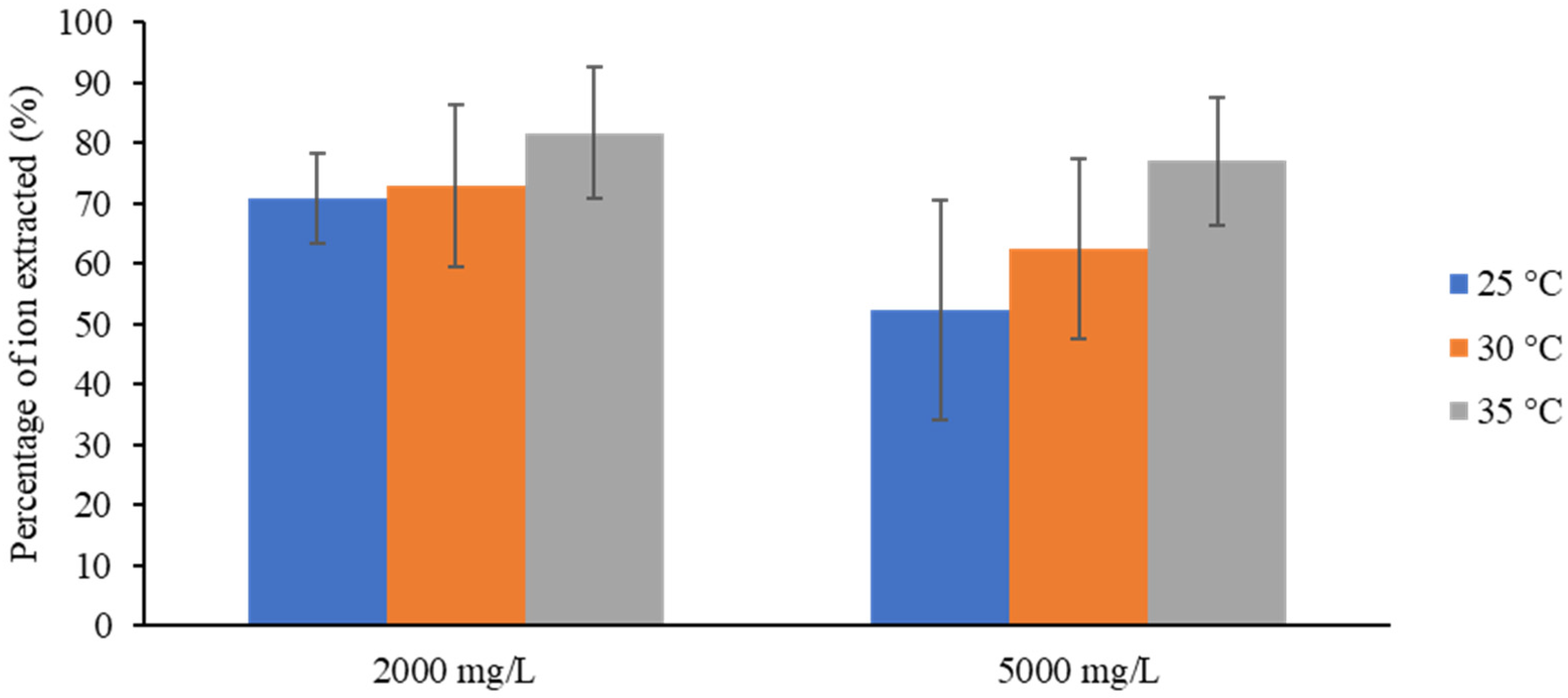
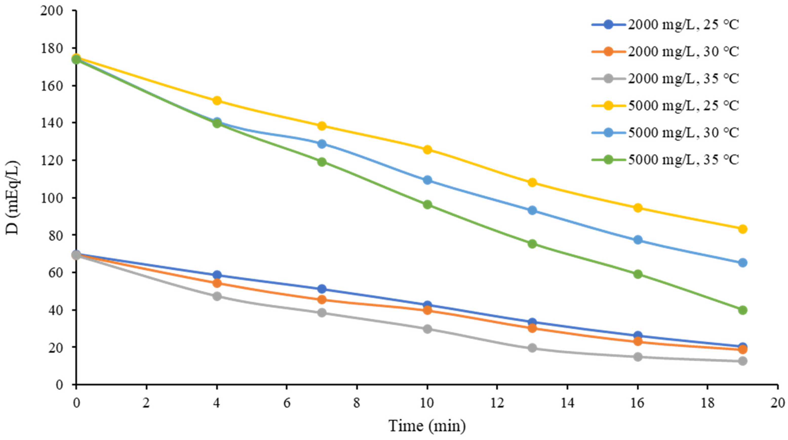
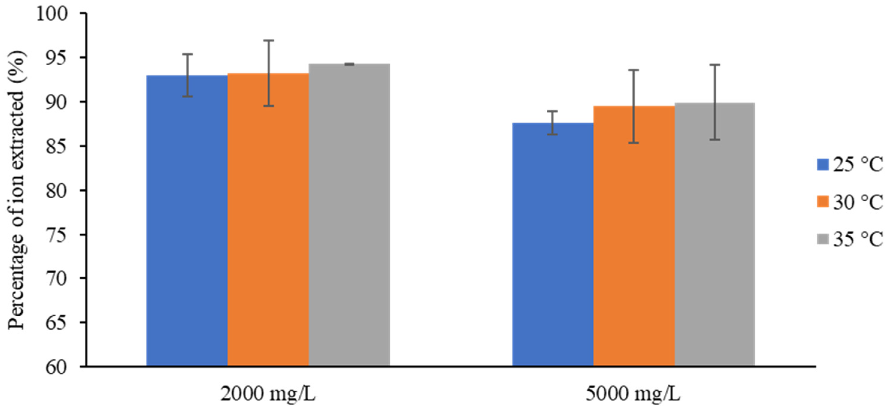
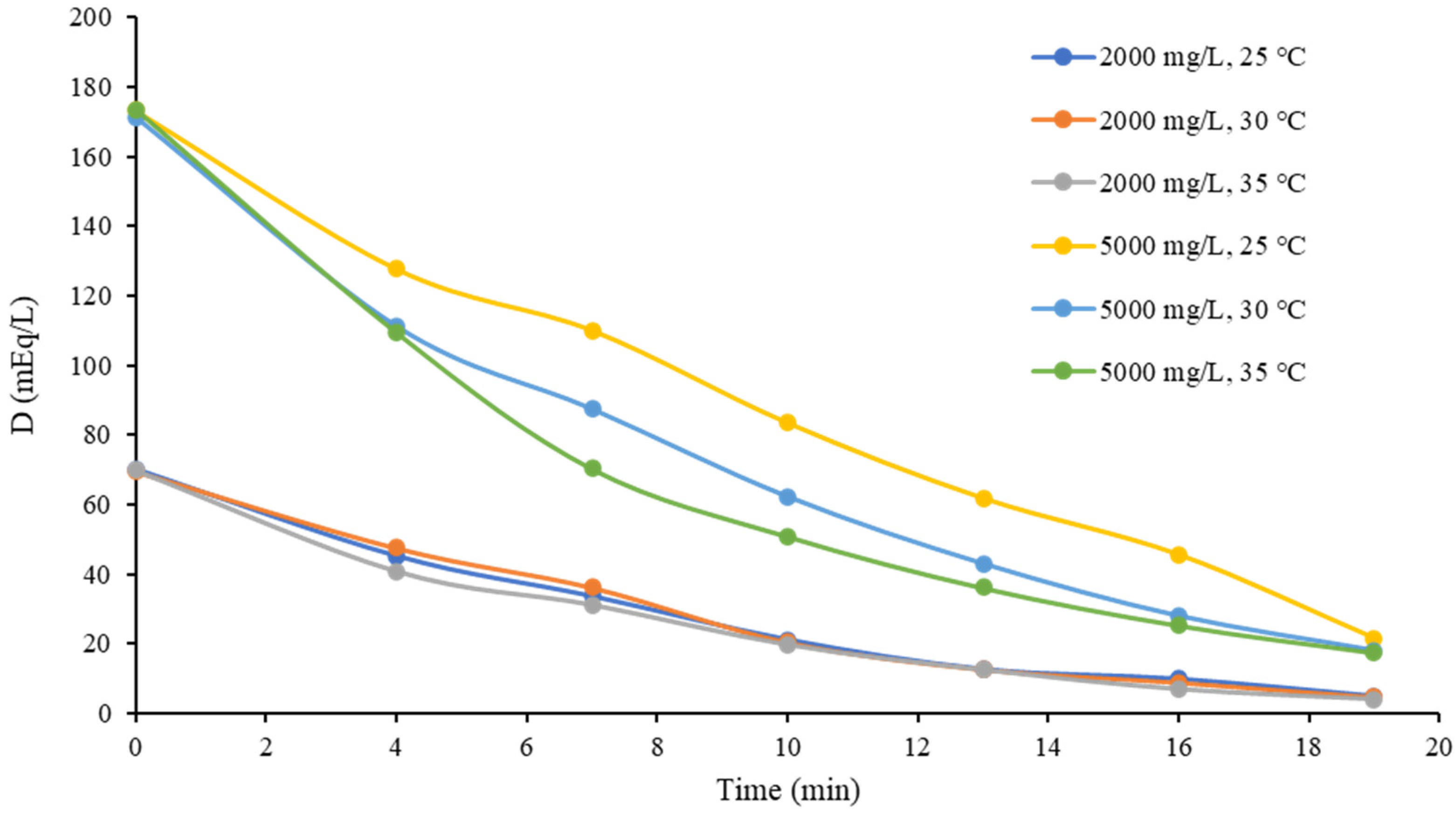
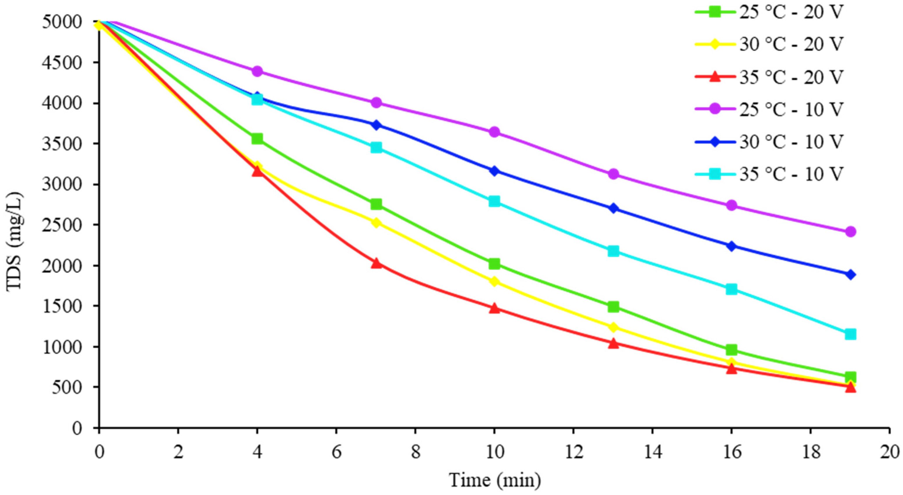
3.4. Evaluation of the Effect of Temperature on Removal Efficiency

The following section discusses the impact of the feed water temperature on ion removal. The comparison was made over the two applied voltages (10 and 20 V) and the two inlet concentrations (2000 and 5000 mg/L). It should be clarified that, in all of the tests, no differences were detected in the temperatures of the diluted streams compared to the concentrated streams at every sampling. The resulting efficiencies in the tests at 5000 mg/L and 2000 mg/L with 10 V are compiled in Figure 6 as a function of temperature.

Both solutions showed an increase in the percentage of ions extracted as the feed water temperature increased. There were improvements of 10.83% and 24.69% as the temperature increased by 10 °C in the 2000 and 5000 mg/L solutions, respectively. Other studies [21,27] in which a similar method was replicated stated that the increase in diffusivity and ion mobility with increasing temperature was the factor that defined the behavior of the removal efficiency in the process. In addition, the dilatation in the membrane network enhanced the diffusion of ions over the membrane material [28].

To compare how the changes in temperature and inlet concentration affected the process, the evolution of the diluate stream concentration (in mEq/L) during the 10 V tests is shown in Figure 7.

It is remarkable that the concentration in the 2000 mg/L (~69 mEq/L) tests decreased at a lower rate compared to the 5000 mg/L (~173 mEq/L) cases, since the former tended to be less pronounced. This behavior was due the fact that concentration polarization started to take place in the membrane boundary layer [29]. In addition, this explanation can be the reason for why the cases with the higher initial concentration (5000 mg/L) presented a more noticeable effect of temperature, since their curves had a space between them that was larger than that in the 2000 mg/L cases. The latter could be quantified by establishing a difference between the concentrations in the 35 and 25 °C test (D_25°C–D_35°C), as shown in

Table 6. Differences between the diluate stream concentrations in the 25 and 35 °C tests.

Time (min)	D25°C–D35°C (mEq/L)
	2000 mg/L		5000 mg/L
	10 V	20 V	10 V	20 V
0	0	0	0	0
4	11.0773	4.4042	12.1228	18.2840
7	12.5120	2.4914	19.1520	39.7605
10	12.6233	1.4683	29.5547	32.5869
13	13.9693	0.2445	32.6684	25.6693
16	11.1218	2.9587	35.5453	20.2417
19	7.6962	0.9122	43.4715	4.0484
Average	11.5	2.08	28.7524	23.4318

.

Table 6 presents the difference D_25°C–D_35°C at every measurement time and the averages of all cases. It is noticeable that the average concentration difference in the 5000 mg/L tests was larger compared to that in the 2000 mg/L tests.

Corresponding to the 20 V tests, the trend in the removal efficiency was similar to that in the experiments in the previous section. In Figure 8, the percentages of ions extracted for every case at 20 V are shown. It can be seen that the increase in salt separation with increasing temperature was less pronounced—it was around 1% for both feed concentrations. In addition, the applied voltage was sufficient to remove salts beyond 85%; thus, a voltage greater than 20 V no longer has much sensitivity to temperature in these ranges of operation.

This also can be noticed in Figure 9, where the 20 V TDS diluate concentration curves were very close to each other. Recalling the averages calculated in Table 6, the differences in the 20 V tests (2.08 and 23.43 mEq/L) were lower than those in the 10 V tests (11.5 and 28.75 mEq/L). This can be attributed once again to the concentration polarization and the influence of electroosmotic flux, since electroosmosis causes an increase in water transport over the membrane, which limits ion migration from the diluate to the concentrated stream and stops the decreasing tendency of its concentration because water is transported proportionally through the membrane [29,30].

3.5. Comparison with NOM-127 Standards

Another important point of comparison is the salinity of the diluate water with respect to the Official Mexican Standard (NOM-127-SSA1-1994). Ref [31] indicates 1000 mg/L TDS as a permissible limit for water for human consumption. Figure 10 and Figure 11 show how TDS was eliminated over time for the samples at the three inlet temperatures and the two voltages.

As expected, the 20 V tests were the quickest to achieve concentrations of less than 1000 mg/L TDS for diluate water, with the 35 °C samples being the first to meet this parameter. With the 2000 and 5000 mg/L samples, this removal was achieved in approximately 7.7 and 13.4 min, respectively. From this perspective, it is also possible to detect how the temperature did not produce too much of an effect when working under these voltage conditions, since the curves were almost together and the final concentration was almost the same in the final portion. Finally, in

Table 7. Mass balance of the experiments at 2000 mg/L, 35 °C, and 20 V.

	Feed Water	Diluate Water	Concentrated Water		Feed Water	Diluate Water	Concentrated Water
Cations (meq/L)				Anions (meq/L)
Ca	1.19	0.07	2.05	HCO3	0.14	0.01	0.23
Mg	5.66	0.32	9.69	SO4	3.27	0.19	5.6
Na	27.04	1.55	46.37	Cl	31.47	1.81	53.95
K	0.59	0.03	1.01	F	0.01	0	0.01
NH4	0.012	0	0	NO3	0.01	0	0.02
Ba	0.018	0	0	PO4	0.05	0	0.09
Sr	0.019	0	0	B	0.05	0	0.09
Total	34.52	1.97	59.12	Total	35	2.01	59.99

and

Table 8. Mass Balance of the experiments at 5000 mg/L, 35 °C, and 20 V.

	Feed Water	Diluate Water	Concentrated Water		Feed Water	Diluate Water	Concentrated Water
Cations (meq/L)				Anions (meq/L)
Ca	2.96	0.3	5.13	HCO3	0.34	0.03	0.59
Mg	14.03	1.42	24.35	SO4	8.11	0.82	14.04
Na	67.13	6.77	116.26	Cl	78.12	7.87	135.29
K	1.46	0.15	2.54	F	0.01	0	0.02
NH4	0	0	0.01	NO3	0.02	0	0.03
Ba	0	0	0	PO4	0.12	0.02	0.21
Sr	0	0	0.01	B	0.14	0.01	0.13
Total	85.58	8.64	148.3	Total	86.84	8.76	150.18

, the mass balances for the cases that attained the highest percentages of ions extracted are shown for each initial concentration.

3.6. Energy Demand of the Process

It is relevant to calculate the differences in energy consumption in the different tests in order to know how profitable it is to increase the voltage and temperature of the process, so the cases were compared again to see how the energy consumption behaved.

Table 9. Average energy demand of the pump and rectifier for each test.

Arrangement	Heating (kWh)		Pump (kWh)		Rectifier (kWh)
	10 V	20 V	10 V	20 V	10 V	20 V
2000 mg/L–25 °C	0.08	0.08	0.0250	0.0260	0.0125	0.0214
2000 mg/L–30 °C	0.13	0.13	0.0245	0.0253	0.0125	0.0214
2000 mg/L–35 °C	0.22	0.22	0.0245	0.0253	0.0125	0.0214
5000 mg/L–25 °C	0.16	0.16	0.0263	0.0263	0.0173	0.0312
5000 mg/L–30 °C	0.24	0.24	0.0256	0.0257	0.0173	0.0312
5000 mg/L–35 °C	0.38	0.38	0.0255	0.0255	0.0173	0.0312

shows the results corresponding to the energy used by the heating of the water, pumping equipment, and the rectifier, and

Table 10. Average total energy demand for each test.

Arrangement	10 V (kWh)	20 V (kWh)	Increased Energy Consumption (%)
2000 mg/L–25 °C	0.1175	0.1274	8.42
2000 mg/L–30 °C	0.167	0.1767	5.8
2000 mg/L–35 °C	0.257	0.2667	3.77
5000 mg/L–25 °C	0.2036	0.2175	6.83
5000 mg/L–30 °C	0.2829	0.2969	4.95
5000 mg/L–35 °C	0.4228	0.4367	3.29

shows the total consumption.

In all cases, the energy consumption or expenditure was higher in the tests in which 20 V was applied, since the rectifier required more energy in order to produce the power demand for the imposed current. On the other hand, the energy consumed by the pump decreased as the temperature rose, since the opposition of the BW to the fluid to be transported by the pump equipment was reduced [32]. The tests at 5000 mg/L in the feed were more energy demanding than those at lower concentrations because more energy was required to keep the rectifiers at the set voltage, while the pumps also needed more energy.

3.7. Water Cost Evaluation

The costs of water production in desalination vary in a wide range; this depends on different factors, among which the following are highlighted: the quality of the source water, the quality of the demanded water, and the plant capacity, among others [33]. To estimate the energy cost of the process, the water quality demanded was set to the one established by NOM-127-SSA1-1994. For all cases, the time required to reach that concentration was estimated and projected for 24 h of operation; this was in order to compute the energy consumption spread over an entire day. Finally, the cost per cubic meter of water was obtained from the average basic consumption rate given by Federal Commission of Electricity (CFE) [34]. The heating consumption was not considered in order to keep the effect of the increase in temperature on the cost.

Table 11. Energy cost per cubic meter of water.

Arrangement	Production Energy Cost (USD/m3)
	10 V	20 V
2000 mg/L–25 °C	0.52	0.66
2000 mg/L–30 °C	0.51	0.65
2000 mg/L–35 °C	0.51	0.65
5000 mg/L–25 °C	0.61	0.80
5000 mg/L–30 °C	0.60	0.79
5000 mg/L–35 °C	0.59	0.78

summarizes the energy costs of production per cubic meter of water for all arrangements.

The above data show that the price increases if the feed stream is more concentrated. On the other hand, as expected, it is observed for tests at the same voltage that the cost decreases with the increase in temperature; the same trend is detectable at 20 V. Lower-voltage operations are cheaper than their counterparts; however, fewer cubic meters are desalinated. The price range of water in desalination processes is reported to be between 0.48 and 3.59 USD/m³ [35]. This production is also below the prices of electrodialysis from recent years (0.75 USD/m³) [36]. In addition, Dévora et al. [33] reported that the price of water processed with reverse osmosis is around 0.6 USD/m³.

4. Conclusions

It is concluded that increases in temperature and voltage are parameters that positively affect the salt removal efficiency of the EDR process. The limiting current density for the 2000 mg/L sample was between 18 and 19 volts, and for the 5000 mg/L sample, it was between 11 and 12.5 volts; both processes were conducted at a flow rate of 60 L/h.

It was found that a voltage of 20 V and a temperature of 35 °C are the best combination of operating parameters for achieving the highest levels of salt removal at 89.5% and 94.24% for salinities of 5000 and 2000 mg/L, respectively. The time to reach the concentration suitable for human consumption—500 mg/L according to NOM-127-SSA1-1994—in the 5000 mg/L concentration test at 20 V and 35 °C was 13 min, while in the 2000 mg/L test at 20 V and 35 °C, it was 7 min.

Energy consumption was reduced throughout the process with the increase in temperature: 1.33% and 1.47% for the 2000 and 5000 mg/L TDS arrays at 10 V; the savings at 20 V were 1.83% and 1.39% at 2000 and 5000 mg/L TDS, respectively. All of the energy savings had an impact on the cost of production, making it more economical; the price range was between 0.52 and 0.78 USD/m³. The present study demonstrates the importance of desalination by membrane systems and the application of temperature, as the economic feasibility and time optimization make these profitable. This also represents an alternative solution for scaling up EDR processes for coastal communities that do not have water and energy by providing sustainable water.

References

1. Marshall, S.J. Hydrology. In Reference Module in Earth Systems and Environmental Sciences; Elsevier: Amsterdam, The Netherlands, 2013. [Google Scholar] [CrossRef]
2. Rijsberman, F.R. Water scarcity: Fact or fiction? Agric. Water Manag. 2006, 80, 5–22. [Google Scholar] [CrossRef] [Green Version]
3. Comisión Nacional Del Agua. In Estadísticas del Agua en México, 2017 ed.; Secretaria de Medio Ambiente y Recursos Naturales: Mexico City, Mexico, 2017; p. 291.
4. Medina, M.R.; Saavedra, R.M.; Montaño, M.M.; Gurrola, J.C. Vulnerabilidad a la intrusión marina de acuíferos costeros en el Pacífico Norte Mexicano; un caso, el acuífero costa de Hermosillo, Sonora, México. Rev. Lat.-Am. Hidrogeol. 2002, 2, 31–52. [Google Scholar] [CrossRef]
5. Rodríguez-López, J.; Robles-Lizárraga, A.; Encinas-Guzmán, M.I.; Correa-Díaz, F.; Dévora-Isiordia, G.E. Assessment of fixed, single-axis, and dual-axis photovoltaic systems applied to a reverse osmosis desalination process in northwest Mexico. Desalination Water Treat. 2021, 234, 399–407. [Google Scholar] [CrossRef]
6. Monreal, R.; Castillo, J.; Rangel, M.; Morales, M.; Oroz, L.A.; Valenzuela, H. La intrusión salina en el acuífero de la costa de hermosillo, Sonora. In Proceedings of the Acta de Sesiones de la XXIV Convención Internacional de la Asociación de Ingenieros de Minas Metalurgistas y Geólogos de México, Acapulco, Mexico, 17–20 October 2001; pp. 93–98. [Google Scholar]
7. Gillam, W.S.; McCoy, W.H. Desalination Research and Water Resources. Princ. Desalination 1967, 2, 1–20. [Google Scholar] [CrossRef]
8. Robles-Lizárraga, A.; Martínez-Macías, M.d.R.; Encinas-Guzmán, M.I.; Larraguibel-Aganza, O.d.J.; Rodríguez-López, J.; Dévora-Isiordia, G.E. Design of reverse osmosis desalination plant in Puerto Peñasco, Sonora, México. Desalination Water Treat. 2020, 175, 1–10. [Google Scholar] [CrossRef]
9. Belessiotis, V.; Kalogirou, S.; Delyannis, E. Chapter one—Desalination methods and technologies—Water and energy. In Thermal Solar Desalination; Academic Press: Cambridge, MA, USA, 2016; pp. 1–19. [Google Scholar] [CrossRef]
10. Ruan, G.; Wang, M.; An, Z.; Xu, G.; Ge, Y.; Zhao, H. Progress and Perspectives of Desalination in China. Membranes 2021, 11, 206. [Google Scholar] [CrossRef]
11. Strathmann, H. Chapter one—Overview of ion-exchange membrane processes. In Membrane Science and Technology; Elsevier: Amsterdam, The Netherlands, 2004; Volume 9, pp. 1–22. [Google Scholar] [CrossRef]
12. Strathmann, H. Assessment of electrodialysis water desalination process costs. In Proceedings of the International Conference on Desalination Costing, Limassol, Cyprus, 6 December 2004; pp. 32–54. [Google Scholar]
13. Katz, W.E. The electrodialysis reversal (EDR) process. Desalination 1979, 28, 31–40. [Google Scholar] [CrossRef]
14. Armendariz-Ontiveros, M.M.; Álvarez-Sánchez, J.; Dévora-Isiordia, G.E.; García, A.; Fimbres Weihs, G.A.; Dévora-Isiordia, G.E. Effect of seawater variability on endemic bacterial biofouling of a reverse osmosis membrane coated with iron nanoparticles (FeNPs). Chem. Eng. Sci. 2020, 223, 115753. [Google Scholar] [CrossRef]
15. Baker, R.W. Ion Exchange membrane processes—Electrodialysis. In Membrane Technology and Applications; John Wiley & Sons: Hoboken, NJ, USA, 2004; pp. 393–423. [Google Scholar]
16. Encinas-Guzmán, M.I.; Robles-Lizárraga, A.; Rodríguez-López, J.; Dévora-Isiordia, G.E. Economic evaluation of reverse osmosis brine evaporation: Environmental management in Mexico. Rev. Int. Contam. Ambient. 2021, 37, 319–327. [Google Scholar]
17. Honarparvar, S.; Zhang, X.; Chen, T.; Alborzi, A.; Afroz, K.; Reible, D. Frontiers of Membrane Desalination Processes for Brackish Water Treatment: A Review. Membranes 2021, 11, 246. [Google Scholar] [CrossRef]
18. Strathmann, H. Chapter 2 electrochemical and thermodynamic fundamentals. In Membrane Science and Technology; Elsevier: Amsterdam, The Netherlands, 2004; Volume 9, pp. 23–88. [Google Scholar] [CrossRef]
19. Marder, L.; Pérez Herranz, V. Electrodialysis control parameters. In Electrodialysis and Water Reuse, 1st ed.; Springer: Berlin/Heidelberg, Germany, 2014; pp. 25–39. [Google Scholar] [CrossRef]
20. Mavrov, V.; Pusch, W.; Kiminek, O.; Wheelwrigth, S. Concentration polarization and water splitting at electrodialysis membranes. Desalination 1993, 91, 225–252. [Google Scholar] [CrossRef]
21. Benneker, A.M.; Klomp, J.; Lammertink, R.G.H.; Wood, J.A. Influence of temperature gradients on mono- and divalent ion transport in electrodialysis at limiting currents. Desalination 2018, 443, 62–69. [Google Scholar] [CrossRef]
22. Onuki, K. Electro-electrodialysis of hydriodic acid in the presence of iodine at elevated temperature. J. Memb. Sci. 2001, 192, 193–199. [Google Scholar] [CrossRef]
23. López-García, U.; Antaño-López, R.; Orozco, G.; Torres-González, J.; Castañeda, F. Comparison on Nine Membrane Pairs for Electrodialytic Removal of Nitrate Ions. J. Water Resour. Prot. 2011, 3, 387–397. [Google Scholar] [CrossRef] [Green Version]
24. Kucera, J. Basic terms and definitions. In Reverse Osmosis; John Wiley & Sons, Inc.: Hoboken, NJ, USA, 2015; pp. 25–48. [Google Scholar]
25. Singh, R. Desalination and on-site energy for groundwater treatment in developing countries using fuel cells. In Emerging Membrane Technology for Sustainable Water Treatment; Elsevier: Amsterdam, The Netherlands, 2016; pp. 135–162. [Google Scholar]
26. Walker, W.S.; Kim, Y.; Lawler, D.F. Treatment of model inland brackish groundwater reverse osmosis concentrate with electrodialysis—Part II: Sensitivity to voltage application and membranes. Desalination 2014, 345, 128–135. [Google Scholar] [CrossRef]
27. Gherasim, C.-V.; Křivčík, J.; Mikulášek, P. Investigation of batch electrodialysis process for removal of lead ions from aqueous solutions. Chem. Eng. J. 2014, 256, 324–334. [Google Scholar] [CrossRef]
28. Amor, Z.; Malki, S.; Taky, M.; Bariou, B.; Mameri, N.; Elmidaoui, A. Optimization of fluoride removal from brackish water by electrodialysis. Desalination 1998, 120, 263–271. [Google Scholar] [CrossRef]
29. Banasiak, L.J.; Kruttschnitt, T.W.; Schäfer, A.I. Desalination using electrodialysis as a function of voltage and salt concentration. Desalination 2007, 205, 38–46. [Google Scholar] [CrossRef] [Green Version]
30. Galama, A.H.; Saakes, M.; Bruning, H.; Rijnaarts, H.H.M.; Post, J.W. Seawater predesalination with electrodialysis. Desalination 2014, 342, 61–69. [Google Scholar] [CrossRef]
31. NOM-127-SSA1-1994, Salud Ambiental. Agua para uso y consumo humano. Límites permisibles de calidad y tratamientos a que debe someterse el agua para su potabilización. In Diario Oficial de la Federación; Secretaría de Salud: Mexico City, Mexico, 2000. [Google Scholar]
32. Leitz, F.B.; Accomazzo, M.A.; McRae, W.A. High temperature electrodialysis. Desalination 1974, 14, 33–41. [Google Scholar] [CrossRef]
33. Dévora-Isiordia, G.E.; González-Enríquez, R.; Ruiz-Cruz, S. Evaluación de procesos de desalinización y su desarrollo en México. Tecnol. Cienc. Agua 2013, 4, 27–46. [Google Scholar]
34. CFE. Tarifas. Available online: https://app.cfe.mx/Aplicaciones/CCFE/Tarifas/Tarifas/tarifas_casa.asp (accessed on 15 April 2021).
35. Karagiannis, I.C.; Soldatos, P.G. Water desalination cost literature: Review and assessment. Desalination 2008, 223, 448–456. [Google Scholar] [CrossRef]
36. Al-Amshawee, S.; Yunus, M.Y.B.M.; Azoddein, A.A.M.; Hassell, D.G.; Dakhil, I.H.; Hasan, H.A. Electrodial-ysis desalination for water and wastewater: A review. Chem. Eng. J. 2020, 380, 122231. [Google Scholar] [CrossRef]
Figure 1. Diagram of the desalination principle for electrodialysis [12].
Separations 08 00229 g001
Figure 2. Piping and instrumentation diagram of the electrodialysis equipment with a rate of 50 L/h.
Separations 08 00229 g002
Figure 3. Limiting current density tests for the 2000 and 5000 mg/L samples.
Separations 08 00229 g003
Figure 4. The evolution of the TDS in tests of 2000 mg/L TDS.
Separations 08 00229 g004
Figure 5. The evolution of the TDS in tests of 5000 mg/L TDS.
Separations 08 00229 g005
Figure 6. Effect of the inlet temperature on removal efficiency in experiments at 10 V.
Separations 08 00229 g006
Figure 7. Diluate stream concentration over time at 10 V.
Separations 08 00229 g007
Figure 8. Effect of inlet temperature on removal efficiency in the experiments at 20 V.
Separations 08 00229 g008
Figure 9. Diluate stream concentration over time at 20 V.
Separations 08 00229 g009
Figure 10. Desalination of the 2000 mg/L TDS samples at the chosen temperatures and initial concentrations.
Separations 08 00229 g010
Figure 11. Desalination of the 5000 mg/L TDS samples at the chosen temperatures and initial concentrations.
Separations 08 00229 g011