Numerical Investigation of 2D Ordered Pillar Array Columns: An Algorithm of Unit-Cell Automatic Generation and the Corresponding CFD Simulation

Abstract

This paper presents a numerical investigation into the generation of 2D ordered pillar array columns for liquid chromatography columns, focusing on the development of an algorithm for the automatic creation of unit-cell morphologies and their subsequent computational fluid dynamics (CFD) simulation. The algorithm is developed to incorporate functional and operational constraints, which ensure that the generated structures are permeable and suitable for chromatographic separations. The functional constraints include the principal pathway and no dry void constraints, while the operational constraints involve symmetry and porosity thresholds. The algorithm’s efficacy is demonstrated with a reduction rate of 97.8% for order 5 matrices. CFD simulations of the generated morphologies reveal that the homogeneity of the fluid velocity profile within the unit cell is a key determinant of separation performance, suggesting that refining the resolution of discrete unit cells could enhance separation efficiency. Future work will explore the inclusion of more complex morphologies and the impact of particle shape and size on separation efficiency.

1. Introduction

Over the past two decades, ordered stationary phases have gradually developed as a superior alternative, offering improved performance. Knox pointed out that it was possible to obtain significant improvements in the reduced plate height by providing a high degree of homogeneity in the structure [1]. In 1998, He et al. first fabricated ordered pillar array columns (PACs) for 2D liquid chromatography chips using deep reactive ion etching, opening up new possibilities for high-performance chromatography [2]. Op De Beeck et al. provided a theoretical foundation for PACs constructed from diamond-shaped, radially elongated pillars, concluding that such arrays could significantly reduce the minimum plate height by a factor of 6 [3]. De Smet et al. [4] and Gzil et al. [5] further developed this concept using finite element analysis and evaluated several possible PAC configurations with different particle shapes, demonstrating that the separation impedance of ordered diamond pillars was 40% lower than that of circular and hexagonal pillar arrays. Dolamore et al. also assessed the impact of bed configuration on 3D ordered packing via CFD simulations, where non-spherical particles can both reduce mobile-phase band broadening and increase permeability compared with spheres in ordered packed beds [6].

This previous work followed a “top-down” approach, with focus on specific morphologies as directed by the intuition of the authors, e.g., radially elongated diamond pillars for PACs [7], triply periodic minimal surfaces [8,9] or other 2- or 3D structures [10,11]. This approach leaves the morphology solutions space largely unexplored, significantly restraining investigation of potentially strong structures that could find application in the chromatography space. In this regard, a “bottom-up” approach to morphology generation that could explore the entire morphology space has the potential to uncover solutions that are not restricted or biassed by human instinct and perceptions.

A tool for morphology generation based on an automated algorithm that is unbiased by human stereotypes, opinions, and misconceptions has the potential to support bespoke regular morphologies designed to minimize band broadening and offer emphasized retentive properties for certain analytes to further enhance separations. On the other hand, the modelling of chromatographic stationary phases under non-retentive conditions is an economical starting point for key considerations such as permeability and band broadening [6,8,12,13,14,15,16,17], simplifying the computations of the fluid flow and mass transfer properties by discounting for retentive properties.

In this work, a numerical algorithm was designed and optimized to explore the entire design space of possible 2D configurations for PACs. PACs morphologies were idealized as a matrix defining the regions of the mobile and the solid phases. In particular, this work aims to do the following: (1) to develop an algorithm to generate 2D PAC ordered morphologies; (2) to develop constraints to ensure that the generated structures can be applied for chromatographic systems and limit the total number of generated morphologies; (3) to evaluate the performance of the developed constraints; (4) to analyze the separation performance of generated structures and induce a general trend to improve column performance.

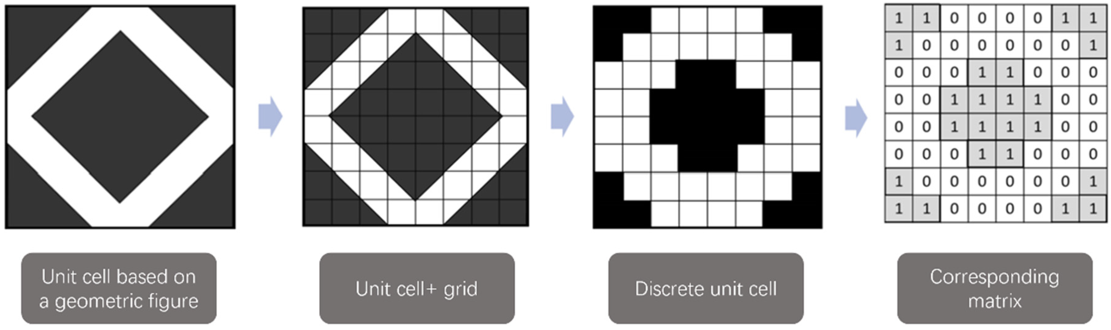
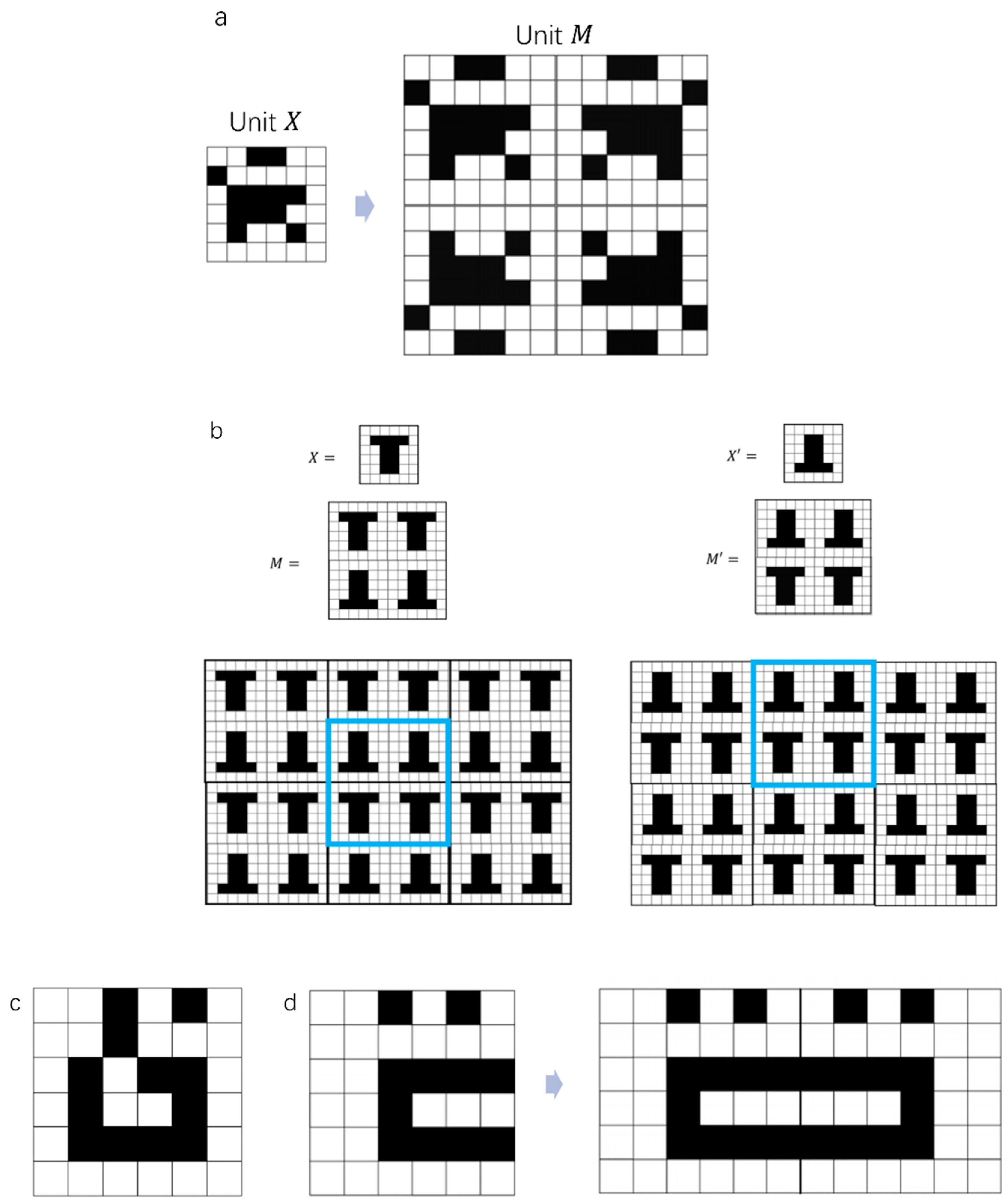
2. Numerical Algorithm for the Generation of PAC Morphologies

A numerical algorithm was designed to generate all possible 2D PACs at a given resolution. To explore the entire domain space of 2D morphologies, the unit cell is represented as an array of discrete pixels. For example, Figure 1 showcases a generic square pillar unit cell in an 8 × 8 grid. Each pixel in the unit cell can take two possible values, with white pixels representing areas available for fluid flow (and assigned a value of 0 in the associated matrix), while black pixels indicate areas occupied by the solid phase (and assigned a value of 1 in the associated matrix). The resolution of the discrete unit cell is increased by reducing the pixel size, with the side result of greatly increasing the computational resources needed for the exploration and generation of all possible morphologies.

The number of possible structures increases exponentially with the grid definition according to $2^{\left(n^2\right)}$, with n corresponding to the resolution. Because of this, attempting to generate all possible discrete unit cells from high-definition grids is particularly time and resource intensive. Rather than using single elements to generate a new matrix, a column-based method is introduced to construct the basic matrix $X$ (Supporting Information Section S1). Appropriate constraints were developed and imposed on the numerical algorithm to reduce by up to 2 orders of magnitude the domain space of the possible matrix permutations.

Symmetry constraint: Ordered and periodic solid phases provide higher performances in terms of separation than disordered ones, owing to the regularity they confer on the flow [4,5,6,18,19]. Due to the 2D nature of the problem, the ordered unit cell was generated by symmetrical reflection about the x and y axes, creating a 2n × 2n unit cell from a less computationally intensive n × n matrix $X$ (Figure 2a). This aspect crucially decreases the possible combinations of morphologies by a factor of $2^{\left({4n}^2\right)}/2^{\left(n^2\right)}=2^{\left({3n}^2\right)}$. This procedure also offers an opportunity to further decrease the number of potential permutations. In fact, it is possible for two different units, $X$ and $X^{\prime }$, to create the same array pattern, as demonstrated in Figure 2b. This happens when the two corresponding matrices $X$ and $X^{\prime }$ are symmetric about either their rows or their columns, distinguishing the two cases’ vertical symmetry and horizontal symmetry, respectively, i.e., symmetry with respect to the x or y axis. To do this, the algorithm must not create the second matrix of a pair after the first one has been generated. The details of the implementation of the vertical and horizontal symmetry conditions, denoted as VS and HS, is described in the Supporting Information Section S3.

Fluid flow constraint: Fluid connectivity between the inlet and outlet of the unit cell is a prerequisite for chromatographic functionality. To meet this requirement, the unit cell must include at least one channel that spans the two opposing sides, here defined as principal pathways, and characterized by a continuous sequence of adjacent white pixels bridging the inlet and outlet sides of the unit cell. Fluid flow can only occur through two adjacent white pixels sharing a full side.

No dry void constraint: Morphologies may present voids which cannot be reached by the fluid. These can either be confined within the morphology described by matrix $X$ (Figure 2c) or created by its reflection about the x and y axes to generate the final unit cell (Figure 2d). Both of these conditions were implemented by differentiating between principal and secondary pathways (Supporting Information Section S2). The possible cases for principal and secondary pathways are described in Figure 2 and Figure S1 in the Supporting Information.

Porosity constraint: Finally, the last constraint assumes generation of only those morphologies with a reasonable porosity value between 0.33 and 0.7, in line with conventional chromatographic practices, to ensure a good balance between column capacity and pressure drops [20]. The details of the implementation of the porosity constraint are described in the Supporting Information Section S4.

The discrete unit $X$ is mathematically described as a square matrix $X$ of order $n$, whose elements $x_{i,j}$ correspond to each pixel characterizing the PAC. To reduce the time for creating a full matrix (instead of generation of all $x_{i,j}$ elements) a column addition approach has been employed to generate all possible permutations of the matrix $X$, with a new column $x_{:,j}$ following a previously introduced $x_{:,j-1}$ column to obtain a progressively growing matrix $X_{n\times j}=\left(x_{:,1}\dots x_{:,j}\right)$ (see Supplementary Information). Every time a new column is inserted a check is produced to fulfil the fluid flow and no dry void conditions (here denoted with the acronym PP, Principal Pathways), as well as the vertical and horizontal symmetry (here denoted with VS and HS) and the porosity (PO) constraints, allowing for the early rejection of potential patterns.

3. Computational Fluid Dynamics Methods

3.1. Governing Equations for CFD Models

All morphologies were simulated in COMSOL Multiphysics (version 5.4) using the finite element method to simulate the fluid velocity profile and the dispersion of the tracer in the system. All simulations complied with the Stokes flow condition (Re < 1). The viscosity of the mobile phase was set as the dynamic viscosity of water at room temperature (1 × 10⁻³ Pa·s) and the molecular diffusion coefficient was assumed to be 1 × 10⁻⁹ m²/s as per Gzil et al. [5]. Whilst the CFD models utilized in this work are non-dimensional, by selecting appropriate scale factors the Navier–Stokes (NS) equation can also be non-dimensionalized. The scale factors and the dimensionless variables for the incompressible NS equation are reported in

Table 1. The scaling factors of the incompressible NS equation. The variables with $*$ are the dimensionless variables after transformation.

Dimensional Variables	Scale Factor	Dimensionless Variables
Length $r$	Characteristic length of mobile phase $L$	${\mathit{r}}^{*}={\displaystyle \frac{\mathit{r}}{L}}$ & ${\nabla }^{*}=L·\nabla$
Velocity $u$	Characteristic velocity $U$	$u^{*}={\displaystyle \frac{u}{U}}$
Time $t$	Characteristic time ${\displaystyle \raisebox{1ex}{$L$}\!\left/ \!\raisebox{-1ex}{$U$}\right.}$	$t^{*}={\displaystyle \frac{t}{L/U}}={\displaystyle \frac{t}{\tau }}$
Pressure $p$	Pressure (in Stokes regime) ${\displaystyle \frac{\mu ·U}{L}}$	$p^{*}={\displaystyle \frac{p·L}{\mu ·U}}$
Tracer concentration $c$	Reference concentration $c_{ref}$	$c^{*}=c/c_{ref}$

.

By applying these dimensionless variables into the equation, the NS equation can be transformed as follows:

$${\displaystyle \frac{\partial u^{*}}{\partial t^{*}}}+\left(u^{*}·{\nabla }^{*}\right)u^{*}=-{\displaystyle \frac{1}{Re}}{\nabla }^{*}{p}^{*}+{\displaystyle \frac{1}{Re}}{\nabla }^{*2}{u}^{*}+{\displaystyle \frac{1}{{Fr}^2}}\widehat{g}$$

(1)

where $Fr$ is the Froude number [21] as ${\displaystyle \raisebox{1ex}{$U$}\!\left/ \!\raisebox{-1ex}{$\sqrt{g_{0}L}$}\right.}$. $g_0$ here is the local external force field, e.g., gravity in many applications. In the chromatographic system where the inertial force is much weaker than the viscous term, the inertia term can be neglected, leaving the equation as the creeping motion, which is as follows:

$$Re{\displaystyle \frac{D{u}^{*}}{D{t}^{*}}}=-{\nabla }^{*}{p}^{*}+{\nabla }^{*2}{u}^{*}$$

(2)

For the Stokes flow condition, where the Reynolds number is smaller than 1, the equation can be reduced to the following Stokes equation:

$$-{\nabla }^{*}{p}^{*}+{\nabla }^{*2}{u}^{*}=0$$

(3)

The non-dimensional NS equation is utilized to determine the velocity field within the column. However, to investigate the purification performance, a concentration field of tracer is required. Without considering the interaction between the tracer and the solid phase, there are two types of motions of the tracer in the fluid: advection and diffusion. Advection is the tracer transport process by the fluid bulk motion. Tracers tend to spread or disperse in cases when the distribution of the fluid velocity is not uniform. Another motion of the tracer is molecular diffusion. The tracer in a high-concentration region diffuses to regions with a lower concentration. Compared to advection, the diffusion process is much slower as it is caused by the particle random walk. However, diffusion also has a strong influence on the column separation efficiency if the separation time or the column length is long enough. The advection–diffusion process can be described as the following equation:

$${\displaystyle \frac{\partial c}{\partial t}}+u·\nabla c=D_m{\nabla }^{2}c$$

(4)

where $c$ is the local concentration of the tracer. To non-dimensionlize this equation, a new scaling factor for concentration $c_{ref}$ is involved (see Table S1), which is usually taken as either the feed or the initial values of the adsorbate concentration in solution encountered in the process. The non-dimensional variable $c^{*}$($=c/c_{ref}$) is utilized to transform the equation as follows:

$${\displaystyle \frac{\partial c^{*}}{\partial t^{*}}}+u^{*}·{\nabla }^{*}{c}^{*}={Pe}^{-1}{\nabla }^{*2}{c}^{*}$$

(5)

3.2. Boundary Conditions and Tracer Inlet

Figure 3 represents a stretch of the setting of boundary conditions, where the blue region is the fluid part and the black region is the solid part. Two kinds of boundaries were applied into the model: no-slip boundary and periodic boundary. The periodic boundaries are used to simulate a column with infinite width [22] (red lines in Figure 3). In practice, this corresponds with neglecting the column walls and wall effect. The no-slip boundaries are applied to the fluid–solid interface, where the fluid has zero velocity [23,24].

The inlet concentration of the tracer is assumed to follow a Dirac function $\delta \left(t\right)$ at time 0, with mean and variance equal to 0. This is as follows:

$$\delta \left(t\right)=\left\{\begin{array}{c}+\infty ,t=0\\ 0,t\ne 0\end{array}\right.$$

(6)

The Dirac function can cause a large concentration gradient at the column inlet, which will promote model instability. In order to reduce this problem, a function comprising two hyperbolic tangent terms is adopted, smoothing the gradients preceding and proceeding the solute pulse as follows:

$$c_{in}=C_{max} \left(\tanh \left({\displaystyle \frac{t}{a_1}}+b_1\right)+\tanh \left({\displaystyle \frac{-t}{c_1}}+d_1\right)\right)$$

(7)

where $c_{in}$ is the inlet concentration, $C_{max}$ is the maximum concentration, and $a_1$, $b_1$, $c_1$, and $d_1$ are constants which control the steepness and width of the impulse ($a_1$ = 0.2, $b_1$ = 0.6, $c_1$ = 0.2, and $d_1$ = 0.6).

The time-dependent solver in COMSOL is used for RTD simulation, and the backward differentiation formula (BDF) is used as the time-stepping strategy.

Table 2. Values of $h$ for Peclet numbers of 5 and 20 at different tracer inlet concentrations.

${\mathit{C}}_{\mathit{m}\mathit{a}\mathit{x}}$/mol/L	0.5	1	10	20	40
Pe = 5	0.729	0.729	0.722	0.728	0.732
Pe = 20	0.310	0.308	0.309	0.308	0.309

summarizes the $h$ values of five different $C_{max}$ values with errors smaller than 1% for Peclet numbers of 5 and 20 for an example square pillar. The small errors indicate that the tracer dispersion process is independent of the inlet tracer concentration.

The reduced HETP ($h$) was employed as an indicator of the chromatographic performance of the morphologies, and was calculated from residence time distribution (RTD) simulations following the method described by Jiang and Dimartino [7] and first illustrated by Dolamore et al. [8,13,25]. Briefly, after solving for the steady-flow field, a concentration pulse of an ideal non-retained tracer was introduced at the column inlet and the advection–diffusion process was simulated. The concentration profile at the outlet was then employed to determine the plate height based on the ratio of the increase in the concentration peak variance ($∆{\sigma }^2)$ to the increase in the average retention time ($∆t)$ [26,27]. This is shown as follows:

$$h={\displaystyle \frac{∆{\sigma }^2}{{\left(∆t\right)}^2}}·{\displaystyle \frac{l}{d_h}}$$

(8)

where $l$ and $d_h$ are the length and the hydraulic diameter of the unit cell. The $h$ values were then fitted to the Van Deemter equation to determine the minimum reduced HETP, $h_{min}$.

The permeability was also evaluated in the simulations through the following to estimate the resistance to fluid flow:

$$k=\epsilon {\displaystyle \frac{\widehat{u}\mu }{\frac{dP}{dz}·d_h^2}}$$

(9)

where $k$ is the non-dimensional permeability, $\epsilon$ is the bed porosity, $\widehat{u}$ is the mean flow velocity, $\mu$ is the fluid viscosity, and $dP/dz$ is the pressure drop across the unit cell. The model validation process is reported in Supporting Information Section S5.

3.3. Space Discretization of the CFD Model

For a 2D structure, a number of triangular elements are utilized to cover the entire space domain, as well as some quadrilateral elements close to solid boundaries. The element size governs the overall mesh resolution, where smaller elements yield higher grid density and improved simulation accuracy at the expense of exponentially increasing computational resources and memory requirements. A mesh preliminary independence study is performed to select the proper mesh resolution.

The mesh discretization can be generated by the COMSOL software (version 5.4) automatically. The type and resolution of local details such as corners and boundaries can be altered manually. There are nine levels of the automatically established mesh. Figure 4 illustrates six representative meshes of square pillar configurations, each characterized by two key parameters: (1) average mesh quality, a dimensionless metric quantifying element aspect ratios (with values approaching 1 indicating ideal regular elements) [28]; (2) total element count across the ten-unit cell column structure. Notably, regions containing irregular geometries frequently exhibit a localized mesh quality below 0.1. Quantitative comparisons of these metrics for different resolution levels are systematically tabulated in

Table 3. Mesh quality for the structures in Figure 4 at different resolutions.

Mesh Number	a (Ref)	b	c	d	e	f
Total element number	345,542	138,508	38,246	25,984	15,580	2418
Average mesh quality	0.851	0.845	0.827	0.816	0.792	0.756

.

The separation efficiency of this morphology is evaluated under different meshes. Mesh a (Figure 4a), whose quality value is 0.851, is the highest resolution mesh that the software can automatically generate. This mesh served as a reference to against which compare the influence of resolution on the computed column performance parameters, permeability and $h$. Figure 5 shows the simulation results. In general, the percentage of error compared to the reference value drops almost linearly as the average mesh quality increases. For the three meshes with quality higher than 0.8, both errors of permeability and $h$ (reduced HETP) are smaller than 0.05, indicating that these meshes are able to offer reasonably accurate simulation results. Using these three meshes (b, c, and d), the calculation resources can be significantly diminished as the total element numbers are much smaller than the reference mesh. For example, the simulation time of mesh d is around ten times smaller than the time of the reference mesh. In this work, before running simulations, the mesh quality was checked firstly to ensure that the quality value was higher than 0.8.

4. Results and Discussion

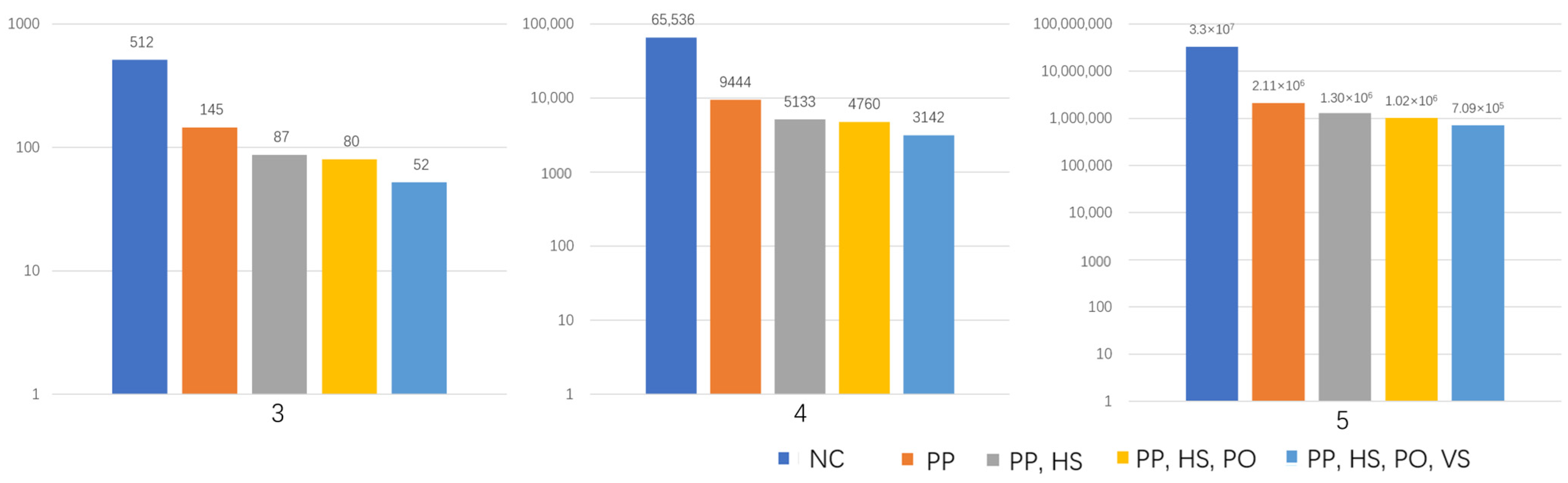
4.1. Impact of the Implementation of the Constraints on Size of Domain Space

Figure 6 reports the number of matrices obtained for the matrices of the orders of 3, 4, and 5 as the constraints are cumulatively implemented. The total reduction rates of the algorithm with all of the constraints are 89.9%, 95.2%, and 97.8% for the orders of 3, 4, and 5, respectively, showing a significant reduction in the number of generated morphologies by the numerical algorithm. Among all of the constraints, the principal pathway (PP) is a critical functional constraint to ensure fluid flow in the generated morphologies. This also produces a significant decrease in potential permutations for matrix $X$, with a relative reduction of 71.7%, 85.6%, and 93.6% for the orders of 3, 4, and 5, respectively, compared to the benchmark case. As the horizontal symmetry (HS) condition is introduced, the number of potential matrices is effectively reduced further down to 11.3%, 6%, and 2.5% for orders 3, 4, and 5, respectively, as also observed for the vertical symmetry (VS) condition with a relative reduction of 5%, 2.5%, and 0.94% for orders 3, 4, and 5, respectively. The decrease associated with the porosity (PO) has a smaller impact at 1.4%, 0.6%, and 0.8% for orders 3, 4, and 5, respectively. While the HS and VS conditions are equivalent, the VS model is implemented after all of the other constraints for practical convenience given the column addition procedure for matrix generation.

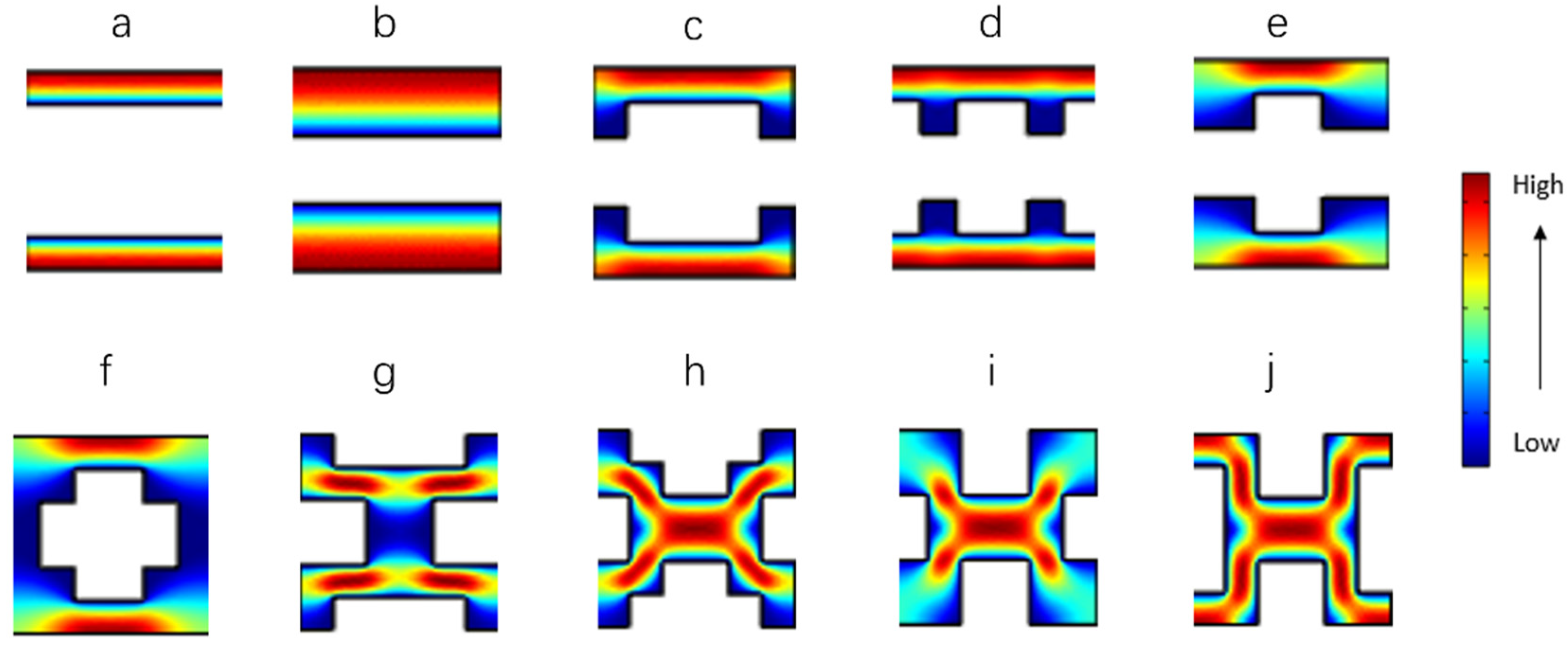
4.2. Effect of Unit-Cell Morphology on Fluid Flow and Band Broadening

As a case study, the separation performance of structures generated for a unit X of order 3 was investigated using CFD simulations to reveal the fluid velocity profiles as well as to estimate the permeability and HETP. Some examples of generated morphologies are reported in Supporting Information Section S6. Figure 7 presents the velocity contour plots for the example unit cells (i.e., local velocity normalized against average interstitial fluid velocity). It is worth mentioning that under laminar flow conditions, different inlet flow rates will not have a significant effect on the velocity contour plots. Two main classes can be distinguished from the structures generated. The first is characterized by a combination of linear channels (Figure 7a,b) or their variations (Figure 7c–e), and in which every fluid channel is not interconnected. The fluid passes through the unit cells with little resistance to the flow, leading to a high non-dimensional permeability (see Table 1). By contrast, the separation efficiency of these morphologies is low, as evidenced by the high $h_{min}$ values in

Table 4. Values of minimum reduced HETP, $h_{min}$, and non-dimensional permeability, $k$, and the corresponding separation impedance, ${\phi }_{min}$, for the morphologies in Figure 7.

	a	b	c	d	e	f	g	h	i	j
Porosity, $\epsilon$	0.33	0.66	0.44	0.44	0.55	0.77	0.55	0.55	0.66	0.55
Permeability, $k$	0.11	0.21	0.12	0.18	0.12	0.08	0.08	0.06	0.04	0.04
Minimum height equivalent to a theoretical plate, $h_{min}$	0.56	0.55	1.71	2.05	1.30	1.77	1.67	1.13	0.61	0.33
Minimum separation impedance, ${\phi }_{min}$	0.94	0.96	10.72	12.27	7.74	30.15	19.17	11.70	6.13	1.49

, probably associated with axial dispersion in the straight channels [25,29,30]. The second class of structures presents interconnecting channels with different lengths of the connecting segment. The normalized fluid velocity is close to zero in those configurations with shorter connections (Figure 7f,g) and shows that the fluid mainly travels along the axial channels rather than through the interconnections, leading to a high degree of axial dispersion and poor performance in terms of HETP (Table 4). Morphologies with wider connections (Figure 7h–j) encourage transverse dispersion, inhibiting axial dispersion and hence performing better in chromatographic terms. The permeability values of these structures are relatively low, corresponding to higher flow resistance on such morphologies compared to the other morphologies (Table 4). In general, an ordered pattern is not a sufficient condition for a homogeneous fluid velocity profile, directly impacting on separation performance. For example, a high proportion of the unit cell in Figure 7h is occupied by flow in the lowest velocity quartile due to the dead zones in the corners and the edges of the unit cell. Figure 7i,j shows a significant increase in fluid homogeneity, which leads to improved performance in terms of the minimum reduced plate height compared to the pattern of Figure 7h (Table 4). This observation agrees with the work of Van Deemter [1,31], which demonstrated that the flow resistance and solute dispersion increased in line with the inhomogeneity of the fluid velocity field. Billen et al. [32] also reported the influence of the homogeneity of the fluid velocity field on band broadening. This observation indicates the need for simulations of unit cells of higher order to reduce the number of dead zones created by the shape corners and the particle edges.

While the computational findings presented in this study provide valuable insights into the design principles of 2D ordered pillar array columns (PACs), the practical realization of these structures remains a critical consideration. The morphologies generated in this work, particularly those with interconnected channels, are amenable to fabrication using existing microfabrication techniques. For instance, deep reactive ion etching, as demonstrated by He et al. [2], has been employed to create high-aspect-ratio pillar arrays with sub-micron precision for microfluidic chromatography chips. Similarly, advancements in two-photon lithography micromachining 3D printing could enable rapid prototyping of complex PAC geometries, including those with non-circular pillar shapes or interconnected pathways [11,33,34,35,36,37].

5. Conclusions

This study presents an algorithm for generating 2D ordered pillar array column (PAC) morphologies using a discrete pixel-based unit-cell approach. By implementing functional constraints (principal pathway and no dry voids) and operational constraints (symmetry and porosity), the algorithm reduces the total number of possible morphologies by up to 97% for order 5 matrices, significantly lowering computational costs. The principal pathway constraint proves most impactful, achieving reductions of 71.7–93.6% across resolutions, while porosity constraints contribute minimally (~1%). Computational fluid dynamics (CFD) simulations reveal two structural classes; Type 1 (linear channels) exhibits high permeability but poor separation efficiency due to axial dispersion, whereas Type 2 (interconnected pathways) enhances transverse dispersion, yielding superior separation performance despite lower permeability. Fluid velocity homogeneity emerges as a critical determinant of efficiency, with refined unit-cell resolutions showing potential to minimize dead zones and further improve performance.

The algorithm proposed is a convenient tool to explore the entire space of regular morphologies for chromatographic beds. Being unbiased by human input, the algorithm has the potential to uncover bespoke morphologies for specific applications requiring precise retentive properties. Building on the foundation established in this study, future extensions accounting for selectivity and loading will broaden the applicability of our approach across a range of scientific and industrial contexts. In pillar array columns, the findings can inform the design and fabrication of next-generation 2D liquid chromatography chips with enhanced performance. For 3D printed columns, the algorithm can guide the optimization of microstructures to improve separation outcomes. Beyond chromatography, the methodology holds promise for applications in heat transfer systems, where tailored structural designs can enhance thermal performance, and in fluid-driven chemical reactions, where optimized geometries can improve reaction efficiency and catalyst support.

References

1. Knox, J.H. Band dispersion in chromatography—A universal expression for the contribution from the mobile zone. J. Chromatogr. A 2002, 960, 7–18. [Google Scholar] [CrossRef]
2. He, B.; Tait, N.; Regnier, F. Fabrication of Nanocolumns for Liquid Chromatography. Anal. Chem. 1998, 70, 3790–3797. [Google Scholar] [CrossRef]
3. Op De Beeck, J.; Callewaert, M.; Ottevaere, H.; Gardeniers, H.; Desmet, G.; De Malsche, W. On the Advantages of Radially Elongated Structures in Microchip-Based Liquid Chromatography. Anal. Chem. 2013, 85, 5207–5212. [Google Scholar] [CrossRef]
4. De Smet, J.; Gzil, P.; Vervoort, N.; Verelst, H.; Baron, G.V.; Desmet, G. On the optimisation of the bed porosity and the particle shape of ordered chromatographic separation media. J. Chromatogr. A 2005, 1073, 43–51. [Google Scholar] [CrossRef]
5. Gzil, P.; De Smet, J.; Vervoort, N.; Verelst, H.; Baron, G.V.; Desmet, G. Computational study of the band broadening in two-dimensional etched packed bed columns for on-chip high-performance liquid chromatography. J. Chromatogr. A 2004, 1030, 53–62. [Google Scholar] [CrossRef]
6. Dolamore, F.; Dimartino, S.; Fee, C.J. Numerical Elucidation of Flow and Dispersion in Ordered Packed Beds: Nonspherical Polygons and the Effect of Particle Overlap on Chromatographic Performance. Anal. Chem. 2019, 91, 15009–15016. [Google Scholar] [CrossRef]
7. Jiang, Q.; Dimartino, S. Simulation of the performance of pillar array columns using the pore-throat ratio as efficiency descriptor. J. Chromatogr. A 2025, 1743, 465704. [Google Scholar] [CrossRef]
8. Dolamore, F.; Houlton, B.; Fee, C.J.; Watson, M.J.; Holland, D.J. A numerical investigation of the hydrodynamic dispersion in triply periodic chromatographic stationary phases. J. Chromatogr. A 2022, 1685, 463637. [Google Scholar] [CrossRef] [PubMed]
9. Lauriola, C.; Venditti, C.; Desmet, G.; Adrover, A. Dispersion properties of triply periodic minimal surface stationary phases for LC: The case of superficial adsorption. J. Chromatogr. A 2025, 1743, 465676. [Google Scholar] [CrossRef] [PubMed]
10. Moussa, A.; Adrover, A.; Desmet, G. Theoretical Prediction of the Ideal Support Shape of 3D-Ordered Liquid Chromatography Supports. Anal. Chem. 2025, 97, 10360–10368. [Google Scholar] [CrossRef] [PubMed]
11. Vankeerberghen, B.; Op de Beeck, J.; Desmet, G. Column-Only Band Broadening in a Porous Shell Radially Elongated Pillar Array Column. Anal. Chem. 2024, 96, 3618–3626. [Google Scholar] [CrossRef] [PubMed]
12. Schure, M.R.; Maier, R.S.; Kroll, D.M.; Ted Davis, H. Simulation of ordered packed beds in chromatography. J. Chromatogr. A 2004, 1031, 79–86. [Google Scholar] [CrossRef] [PubMed]
13. Dolamore, F.; Fee, C.; Dimartino, S. Modelling ordered packed beds of spheres: The importance of bed orientation and the influence of tortuosity on dispersion. J. Chromatogr. A 2018, 1532, 150–160. [Google Scholar] [CrossRef] [PubMed]
14. Schure, M.R.; Maier, R.S. How does column packing microstructure affect column efficiency in liquid chromatography? J. Chromatogr. A 2006, 1126, 58–69. [Google Scholar] [CrossRef]
15. Daneyko, A.; Khirevich, S.; Höltzel, A.; Seidel-Morgenstern, A.; Tallarek, U. From random sphere packings to regular pillar arrays: Effect of the macroscopic confinement on hydrodynamic dispersion. J. Chromatogr. A 2011, 1218, 8231–8248. [Google Scholar] [CrossRef]
16. Schure, M.R.; Maier, R.S.; Kroll, D.M.; Davis, H.T. Simulation of Packed-Bed Chromatography Utilizing High-Resolution Flow Fields: Comparison with Models. Anal. Chem. 2002, 74, 6006–6016. [Google Scholar] [CrossRef]
17. Daneyko, A.; Hlushkou, D.; Khirevich, S.; Tallarek, U. From random sphere packings to regular pillar arrays: Analysis of transverse dispersion. J. Chromatogr. A 2012, 1257, 98–115. [Google Scholar] [CrossRef]
18. Horváth, K.; Lukács, D.; Sepsey, A.; Felinger, A. Effect of particle size distribution on the separation efficiency in liquid chromatography. J. Chromatogr. A 2014, 1361, 203–208. [Google Scholar] [CrossRef]
19. Smits, W.; Nakanishi, K.; Desmet, G. The chromatographic performance of flow-through particles: A computational fluid dynamics study. J. Chromatogr. A 2016, 1429, 166–174. [Google Scholar] [CrossRef]
20. Walls, D.; Walker, J.M. Protein Chromatography; Humana Press: Totowa, NJ, USA, 2017; Volume 1485, ISBN 9781493964109. [Google Scholar]
21. Hager, W.H.; Castro-Orgaz, O. William Froude and the Froude number. J. Hydraul. Eng. 2017, 143, 2516005. [Google Scholar] [CrossRef]
22. Makov, G.; Payne, M.C. Periodic boundary conditions in ab initio calculations. Phys. Rev. B 1995, 51, 4014–4022. [Google Scholar] [CrossRef] [PubMed]
23. Richardson, S. On the no-slip boundary condition. J. Fluid Mech. 1973, 59, 707–719. [Google Scholar] [CrossRef]
24. Sahraoui, M.; Kaviany, M. Slip and no-slip velocity boundary conditions at interface of porous, plain media. Int. J. Heat Mass Transf. 1992, 35, 927–943. [Google Scholar] [CrossRef]
25. Dolamore, F. In Silico Analysis of Flow and Dispersion in Ordered Porous Media; University of Canterbury: Christchurch, New Zealand, 2017. [Google Scholar] [CrossRef]
26. Rimmer, C.E. Heftmann: Chromatography, 6th edition. Fundamentals and applications of chromatography and related differential migration methods. Part A: Fundamentals and techniques. Anal. Bioanal. Chem. 2005, 382, 1447–1448. [Google Scholar] [CrossRef]
27. Poole, C.F. The Essence of Chromatography; Elsevier: Amsterdam, The Netherlands, 2003; ISBN 978-0-444-50198-1. [Google Scholar]
28. Mesh Element Quality and Size. n.d. Available online: https://doc.comsol.com/5.5/doc/com.comsol.help.comsol/comsol_ref_mesh.15.18.html (accessed on 2 May 2025).
29. Caluin, G.J. Dynamics of Chromatography Principles and Theory; CRC Press: Boca Raton, FL, USA, 2017; ISBN 9781315275871. [Google Scholar]
30. Guiochon, G.; Shirazi, D.G.; Felinger, A. Fundamentals of Preparative and Nonlinear Chromatography; Academic Press: Cambridge, MA, USA, 2006; ISBN 978-0-12-370537-2. [Google Scholar]
31. van Deemter, J.J.; Zuiderweg, F.J.; Klinkenberg, A. Commentary from Current Contents ® No. 3 January 19 1981, Longitudinal diffusion and resistance to mass transfer as causes of nonideality in chromatography. Chem. Eng. Sci. 1995, 50, 3867. [Google Scholar] [CrossRef]
32. Billen, J.; Gzil, P.; Vervoort, N.; Baron, G.V.; Desmet, G. Influence of the packing heterogeneity on the performance of liquid chromatography supports. J. Chromatogr. A 2005, 1073, 53–61. [Google Scholar] [CrossRef]
33. Ovsianikov, A.; Chichkov, B.N. Three-dimensional microfabrication by two-photon polymerization technique. Methods Mol. Biol. 2012, 868, 311–325. [Google Scholar] [CrossRef]
34. Gittard, S.D.; Nguyen, A.; Obata, K.; Koroleva, A.; Narayan, R.J.; Chichkov, B.N. Fabrication of microscale medical devices by two-photon polymerization with multiple foci via a spatial light modulator. Biomed. Opt. Express 2011, 2, 3167–3178. [Google Scholar] [CrossRef]
35. Emons, M.; Obata, K.; Binhammer, T.; Ovsianikov, A.; Chichkov, B.N.; Morgner, U. Two-photon polymerization technique with sub-50 nm resolution by sub-10 fs laser pulses. Opt. Mater. Express 2012, 2, 942–947. [Google Scholar] [CrossRef]
36. De Malsche, W.; Op De Beeck, J.; De Bruyne, S.; Gardeniers, H.; Desmet, G. Realization of 1 × 10⁶ Theoretical Plates in Liquid Chromatography Using Very Long Pillar Array Columns. Anal. Chem. 2012, 84, 1214–1219. [Google Scholar] [CrossRef]
37. De Malsche, W.; Eghbali, H.; Clicq, D.; Vangelooven, J.; Gardeniers, H.; Desmet, G. Pressure-Driven Reverse-Phase Liquid Chromatography Separations in Ordered Nonporous Pillar Array Columns. Anal. Chem. 2007, 79, 5915–5926. [Google Scholar] [CrossRef]
38. Karcher, H. The triply periodic minimal surfaces of Alan Schoen and their constant mean curvature companions. Manuscripta Math. 1989, 64, 291–357. [Google Scholar] [CrossRef]
39. Karcher, H.; Polthier, K. Construction of triply periodic minimal surfaces. Philos. Trans. R. Soc. London. Ser. A Math. Phys. Eng. Sci. 1996, 354, 2077–2104. [Google Scholar] [CrossRef]
40. Meeks, W.H., III. The theory of triply periodic minimal surfaces. Indiana Univ. Math. J. 1990, 39, 877–936. [Google Scholar] [CrossRef]
41. Schoen, A.H. Infinite Periodic Minimal Surfaces Without Self-Intersections; National Aeronautics and Space Administration: Washington, DC, USA, 1970; Volume 5541. [Google Scholar]
42. Jung, Y.; Torquato, S. Fluid permeabilities of triply periodic minimal surfaces. Phys. Rev. 2005, 72, 056319. [Google Scholar] [CrossRef]
Figure 1. A generic unit cell for a squared PAC represented as an 8 × 8 matrix.
Separations 12 00184 g001
Figure 2. (a) Example of generation of a symmetric M unit cell of order 2n from a generic morphology X of order n. (b) Representative example of the vertical symmetry condition, with two different units X and X creating the same array pattern after reflection and repetition in the x and y directions (bordered by the blue square). (c) Examples of dry voids contained within matrix X. (d) Examples of dry voids created upon reflection over the x and y axes.
Separations 12 00184 g002
Figure 3. Examples of boundaries in a unit cell. The black area is the stationary phase, and the purple area is the fluid channel. Periodic boundaries, coloured in red, are set at the top and bottom of the cell. The blue arrow shows the direction of the fluid flow.
Separations 12 00184 g003
Figure 4. (af) Six examples of mesh at different resolutions for the same unit cell. Mesh (a) has the highest resolution and is utilized as the reference mesh in the mesh independence testing. Additional data of meshes are reported in Table 3.
Separations 12 00184 g004
Figure 5. (a) Percentage errors of the permeability to the reference simulation of Figure 4; (b) percentage errors of h to the reference. k r e f and h r e f are the permeability and h values of mesh a.
Separations 12 00184 g005
Figure 6. The number of permutations possible in X matrices with orders between 3 and 5 generated from the programme under sequential implementation of constraints. NC: no constraints (orange); PP: principal pathway constraint implemented; HS and VS: horizontal and vertical symmetry constraints implemented, respectively; PO: porosity constraint implemented.
Separations 12 00184 g006
Figure 7. (aj) Examples of morphologies obtained for a unit X of order 3 (unit M of order 6) with the fluid velocity contours obtained by CFD simulations. The local velocity is normalized against average interstitial fluid velocity. Additional data of meshes are reported in Table 4.
Separations 12 00184 g007