Hyphenation of Thermodesorption into GC × GC-TOFMS for Odorous Molecule Detection in Car Materials: Column Sets and Adaptation of Second Column Dimensions to TD Pressure Constraints

Abstract

Vehicle interior air quality is an issue of growing interest among car manufacturers and customers. GC-MS is the benchmark method for the analysis of indoor air or material emissions. It is suitable for the quantification of target pollutants and the most abundant compounds. It fails, however, to uncover the true molecular complexity of these samples. In the present study, we describe the development of a TD-GC × GC-TOFMS method designed to detect polar and potentially odorous molecules in car material emissions. Attention is paid to the hyphenation of the thermodesorber and the gas chromatograph, both at software and hardware levels, and the constraints due to pressure limitations on the thermodesorber (evaluated at 414 kPa/60 psi at the end of the temperature ramp and at 138 kPa/20 psi at rest). A compromise was made for the 2D column length and diameter to balance separation and pressure (50 × 0.18 × 0.18 cm × mm × µm + 60 cm transfer line selected). On various materials, we were able to observe several hundreds of polar molecules, among them were between 75 and 150 odorants per material. This work lays the foundation for the widespread screening of potential odorants in car material emissions.

1. Introduction

Modern cars are very complex constructs made of a wide variety of materials, of which a growing proportion is synthetic. Most of these materials are likely to emit volatile organic compounds (VOCs) in a vehicle’s cabin, constituting a potential nuisance to the drivers and passengers that needs to be monitored [1]. For this reason, several studies relying on gas chromatography (GC) have already been conducted on the molecules present in the car cabins of newly produced cars [2,3,4] or used ones [5,6] or to evaluate the effect of influencing factors (such as vehicle price or driving and parking behaviour) [7,8,9]. The vast majority of the molecules identified in these studies were aliphatic or aromatic hydrocarbons, and their wide diversity often resulted in low-resolution regions in the chromatograms wherein not all peaks could be identified [5,6].

In addition to monitoring vehicle interior air quality (VIAQ), car manufacturers have also developed methods for assessing the odour of these emissions [10,11], such as the series of VDA 276 (Verband der Automobilindustrie, from the combined work of German car manufacturers) [12] and ISO 12219 standards [13]. From this experience, it has been noted that minor changes in the formulation of a material may have a strong impact on the perceived odour of the emissions. Indeed, global odour often results from polar molecules representing a minority in terms of global abundance for this category of materials [14], and a mixture of several odorants can result in an odour very different from the original odorants smelled separately [15,16]. This effect can be emphasised for recycled elements, as the raw materials they are made from inherently have a variable composition, yielding more potentially odorous molecules.

To detect and prevent the presence of malodorous molecules, car manufacturers need analytical tools. Methods relying on human smelling capacity, such as panels [17,18,19,20,21] or GC–olfactometry (GC-O) techniques [22,23,24], exist, but they are very expensive and time-consuming. Panels give no information on molecular composition, and GC-O requires molecules to be separated on the chromatogram so that they can be identified. However, as previously mentioned, typical GC methods fail to fully separate the complex samples that are material emissions. Moreover, odorous polar molecules are rarely detected and are not separated properly from the barely to non-odorous major non-polar compounds in common GC analyses [5,14].

Thus, it is necessary to develop new methods to better detect potentially odorous polar molecules in vehicle interior air. Comprehensive bidimensional gas chromatography (GC × GC), combining two different columns interfaced by a modulator, is a modern analytical technique offering three main improvements in comparison to classical GC: (i) a much higher peak capacity [25], (ii) a structured 2D chromatogram for chemical family identification [26], and (iii) better sensitivity due to refocusing on the modulator [27]. All these elements give GC × GC the potential to separate low-concentration potentially odorous polar molecules from the large number of hydrocarbons present in car material emissions.

In this paper, we present a method combining thermodesorption (TD), comprehensive bidimensional gas chromatography (GC × GC), and time-of-flight mass spectrometry (TOFMS) to undercover the true molecular complexity of material emissions. We aim to create a database of odorants from various car material emissions, focusing on individual molecules instead of clusters belonging to the same family. The present work deals with analytical instrument optimisation and early results towards odorous molecules.

To this day, no tool reliably predicts whether or not a molecule is odorous from its structure alone [21,28,29]. Therefore, any polar molecule may be considered an analyte of interest, and most chemical families must be compatible with analytical conditions. For this broad untargeted screening, the analytical method developed was obtained through an experimental process, with a final goal of observing the largest variety of polar molecules. The present work does not aspire to explain odours by the individually detected odorants alone but to confront, in future works, the global chemical composition of emissions with their global odour perceived by humans.

In the first part, we detail the implementation of our method for the selection of the column set in terms of stationary phase combination. In our instrumental configuration, detailed in the Section 2, the TD was subjected to the total column back pressure at rest and during the whole temperature program. To the best of our knowledge, few experimental TD-GC × GC studies have included aspects on pressure drop [30,31], and none of them have reported compatibility issues between high pressure and TD. As we faced such issues, we provide a discussion in the second part regarding the experiments conducted to adapt the system, through ²D column dimension variations, while trying to maintain the separation performance of the column set selected in the first part.

2. Materials and Methods

2.1. Sample Preparation

All material samples were provided by Renault Group (Guyancourt, France). A wide variety of materials, chosen to be representative, were used for prospective experiments. Among them were 2 ABS (Acrylonitrile Butadiene Styrene), 1 PCABS (Poly Carbonate–ABS), 4 different PP (Poly Propylene), 1 natural and 1 synthetic skin, 6 textiles, and 1 putty. They were complemented by 4 interior air samples. For the Part A experiments, one PP and one synthetic skin were selected as model samples. In Part B, we studied one trunk mat, one Polyurethane foam (PU), and one textile.

The materials were sampled using an internal Renault method adapted from ISO 12219-3 [32]. Discs of materials with a diameter of 6.4 cm were cut from a plate and placed in microchambers MCTE250T, provided by Markes International (Bridgend, UK). The thickness of these materials was variable (a few mm), but the exposed surface was constant at 32 cm². The materials were heated for 20 min at 65 °C at a dew point of 10.4 °C. Under a stream of pure air at 50 mL/min, 1 L of their emissions was collected in Tenax TA tubes (Poly(2,6-diphenylphenylene oxide)), supplied by Sigma-Aldrich (Saint-Quentin-Fallavier, France). The tubes were stored refrigerated and analysed at most two weeks after sampling.

As samples of material emissions were available in limited amounts, system suitability tests were conducted using a mixture of 48 compounds covering a large number of chemical families (see Figure S1 for composition and general peak positions). These samples were prepared by depositing a droplet of standard at the top of a sampling tube, assisted by a gas stream, using the Calibration Solution Loading Rig (CSLR) from Markes International (Bridgend, UK). This method previously achieved a reliable preparation of standard tubes, as well as quantitation for these 48 compounds for a 10 ng deposit, with a limit of detection of the order of 0.1–1 ng [33].

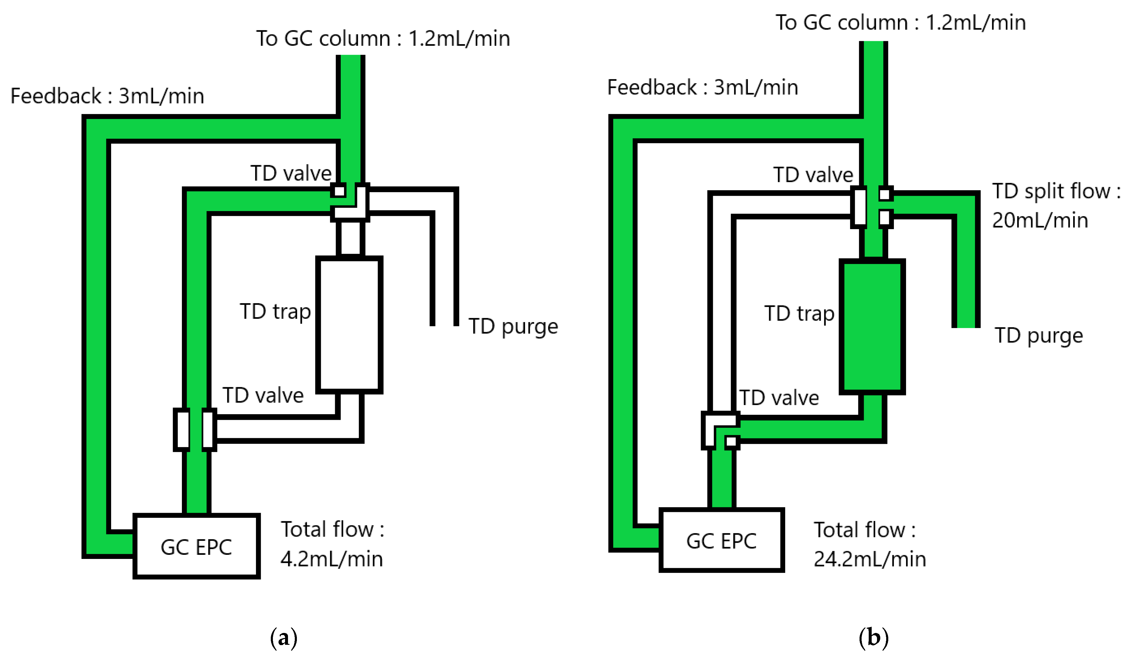
2.2. TD-GC Hyphenation

Once loaded with material emissions, the tubes were analysed using a system composed of a TD100-xr from Markes International (Bridgend, UK) and a GC × GC-TOFMS Pegasus BT4D from LECO (Villepinte, France). The first device was monitored using the software Markes Instrument Control version 2.0.5 and the second one by ChromaTOF version 5.51. The Pegasus BT4D combines a TOFMS detector and a GC device equipped with a modulator and a secondary oven for a potential secondary GC column, thus making it suitable for GC × GC. From the thermodesorber perspective, the association is the same in the GC or GC × GC configuration. According to both instrument manufacturers, this was the first time they had ever been combined.

The global system was supplied with helium as a carrier gas (Alphagaz 1, Air Liquide, France), plugged into both instruments (the TD supply is used only for desorption from sample to trap, which works independently and will therefore be ignored hereafter). The GC carrier gas was pressure-regulated using a GC Electronic Pressure Controller (EPC), then sent into the TD. The TD’s valves maintained a constant flow of 1.2 mL/min into the GC device at all times.

All tubes were desorbed at a flowrate of 50 mL/min and at 270 °C for 10 min (including 3 min to reach the temperature) into a cold trap “General Purpose” U-T11GPC-2S (Markes International, Bridgend, UK) at −30 °C. Then, the cold trap was desorbed at 300 °C for 5 min with a split flow of 20 mL/min and a column inlet flow of 1.2 mL/min with helium as a carrier gas towards the GC × GC through a 150 cm deactivated silica capillary connected to the ¹D column. Split flow was redirected (not represented in Scheme 1) towards the initial sampling tube for recollection (the tube temperature was between 50 and 60 °C).

In this instrumental configuration, the GC EPC controls the pressure for the whole system, and the TD assumes the role of the GC injector, only controlling the split flow during injection (the GC’s own injector is bypassed). Moreover, 3 mL/min of carrier gas is redirected from the TD system to the EPC for pressure feedback. To notify this configuration to the GC instrument, its septum purge time during the injection must be set at 999.99 min, and the feedback flow has to be set with the “septum purge flow” parameter. These carrier gas flows are summarised in Scheme 1.

At the beginning of every analysis, the ChromaTOF software relays the run instructions to the GC device, with the risk of overwriting the previous settings and disturbing communication between the instruments. It also does not allow for the use of methods wherein the septum purge time exceeds the oven program, making only 1000 min programs possible. To solve this issue, we conceived a GC method bearing the gas-monitoring instruction (pressure-controlled constant helium flow of 1.2 mL/min) with septum purge time at 59,999.4 s, a septum purge flow of 3 mL/min, and a fake 1000 min oven program. In later experiments, the GC programs on ChromaTOF had their injector parameter set to “none”. The oven program could still be modified freely, but the septum purge time could not, preventing its overwriting. Thus, the hyphenation of the TD and GC × GC instruments was achieved at a software level.

2.3. Global GC × GC–TOFMS Settings

The different sets of columns used for GC × GC separations are summarised in

Table 1. Stationary phases and dimensions of column sets used in the experiments in Part A; material limitations prevented the use of the same secondary column length; Rxi: Restek; ZB: Phenomenex; DB: Agilent.

Column Set	Short Name	1D phase	2D Dimensions (cm × mm × µm)	2D Phase	Configuration	Modulation Period (s)
Rxi-5MS–ZB-WAX	5–WAX	5% diphenyl	195 × 0.1 × 0.1	100% polyethylene-glycol	Normal	12
Rxi-5MS–ZB-50	5–50	5% diphenyl	175 × 0.1 × 0.1	50% diphenyl	Normal	10
DB-17MS–DB-5	50–5	50% diphenyl	115 × 0.1 × 0.1	5% diphenyl	Reverse	6
Rxi-5MS–DB-210	5–210	5% diphenyl	118 × 0.1 × 0.1	50% trifluoropropyl	Normal	5
ZB-1701–DB-5	1701–5	14%-cyanopropyl-phenyl	84 × 0.1 × 0.1	5% diphenyl	Reverse	2
Rxi-5MS–ZB-1701	5–1701	5% diphenyl	122 × 0.1 × 0.1	14%-cyanopropyl-phenyl	Normal	6

. All the ¹D columns shared the same dimensions: 30 m × 0.25 mm × 0.25 µm. They were provided by Agilent (Les Ulis, France), Restek (Lisses, France) and Phenomenex (Le Pecq, France). The GC × GC was used with a temperature program starting at 40 °C, held for 2 min, and then heated up to 220 °C at 2 °C/min. The temperature of the secondary oven was set 5 °C higher than that of the primary oven, and the modulator temperature was set 15 °C higher than that of the secondary oven. The modulation period of the quad-jet modulator ranged from 2 to 12 s and was adapted to the highest ²D retention time observed to prevent wrapping around. Cold jet time was set at a sixth of the modulation period during preliminary experiments and 0.5 s after.

During the Part B experiments, only the 5–1701 set was used but with various ²D column dimensions. A segment of 7 cm of the ²D column was present in the modulator and the 43 cm remaining in the secondary oven, while the junction with the ¹D column was right at the entrance of the modulator. For convenience, a 60 cm transfer line in deactivated silica matching the diameter of the secondary column was also added between the ²D column and the detector (including 31 cm inside the MS transfer line at 250 °C, the rest being in the secondary oven). The temperature offsets of the secondary oven and modulator with respect to the primary oven were raised to 15 and 30 °C, respectively. The modulation period of the quad-jet modulator ranged from 2 (for 50 cm column) to 4 s (for 100 cm column), consisting of 2 cycles with 0.5 s of cold jet and 0.5 to 1.5 s of hot jet.

The mass spectrometer was used with electronic ionisation at 70 eV, using a scan range of m/z from 45 to 300 at a scan frequency of 200 Hz.

Both acquisition and data processing were conducted using ChromaTOF software. A general Peak Finding (PF) method was employed with an S/N ratio of 500. Most of the time in GC × GC, the ¹D peak of a compound is sampled into several ²D sub-peaks over several modulation periods, resulting in a spot on the colour plot. Such sub-peaks stemming from successive modulations, with similar ²D retention times and identical m/z, are combined by ChromaTOF into a single line of data (individual mass spectra and area are summed). This is what we will call a peak hereafter. Peaks in the aliphatic hydrocarbon elution region were excluded. After that, manual checking was conducted to delete artefact peaks or combine duplicated peaks of successive modulations into a single one. All peaks were attributed based on their mass spectra by comparison with the NIST 2020 database, and they received a score depending on their similarity with the closest match, ranging up to 1000. Peaks with a similarity below 700 were automatically deleted. No changes were made to the proposed attributions.

3. Results

3.1. Part A, Choice of Set of Column

3.1.1. Preliminary Experiments

A wide variety of vehicle material emissions were analysed on the column sets presented in Table 1 in order to screen the largest number of polar molecules. For all the sets, aliphatic hydrocarbons were separated from more polar molecules on our settings. Polar molecule families had variable retention times depending on the secondary column phase, especially for the 5–WAX configuration for benzaldehyde, enones, and lactones, which compelled modulation periods of up to 12 s with some wrapping around still occurring. In this configuration, these excessively large retention times were detrimental to global separation. The 5–50 configuration presented little resolution between polar non-aromatic compounds, making their identification difficult. The 5–210 configuration did not allow for the observation of as many peaks overall as the other configurations. The three remaining column configurations out of the six presented in Table 1 achieved satisfactory separations for preliminary experiments in terms of peak number and separation space occupancy. These configurations consisted of one normal and two reverse configurations: 5–1701, 1701–5, and 50–5.

During these experiments, cold jet duration was left to the default value, being a sixth of the modulation period (and half of hot jet duration). This may have had an impact on peak broadening or a too high retention of high boiling point compounds at the end of the analysis. This should not impact the previous conclusions, as the drawbacks of the rejected configurations were too high. For later experiments, cold jet duration was fixed at 0.5 s. Due to the large variety of studied samples, no further optimisation was made on this parameter to keep the method versatile. For more specific applications, it could be possible to increase cold jet duration at the beginning of the analysis to better trap light compounds and decrease it at the end to release heavy ones better.

From this first screening, two materials were selected as model samples because they covered the largest variety of molecules and situations: a PP emitting a large number of non-polar molecules and a wide variety of diluted polar ones and a synthetic leather emitting a large panel of polar molecules. Thus, these two materials alone were considered sufficient for assessing the separation quality of a column configuration.

3.1.2. Column Phases Selection

The three remaining column configurations needed to be compared using objective numerical criteria. According to our objective, i.e., observing the largest possible number of potentially odorous polar molecules, we decided to use as a performance criterion the number and quality of observed peaks based on similarity criteria regarding the NIST 2020 database. Our hypothesis was that high similarity corresponded to a low-noise and well-resolved peak, regardless of a correct attribution. From our own experience, the true nature of a peak with a similarity above 900 is often close to the proposition, belongs to the same chemical family for a similarity above 800, and may remain undetermined below 800.

The peaks in the aliphatic hydrocarbon elution region, bearing little to no odour and therefore being of no interest in our study, were excluded. Apart from them, all peaks were considered as targets. The number of peaks above each similarity threshold was counted, and the result is presented in Figure 1. The corresponding chromatograms are available in Figure S2. Both materials presented very complex emissions, with several hundreds of relevant peaks detected. These results also stress the contribution of GC × GC over classical GC, as the peak capacity in classical GC could only reach one thousand in ideal and near-theoretical conditions [25,34], meaning that classical GC can only manage the separation of one or two hundred compounds at most.

The same observations could be made for both the mostly non-polar emitting PP and the mostly polar emitting leather: the 5–1701 column configuration yielded the highest number of detected peaks for every similarity threshold. Therefore, a first column with a low-polarity 5%-diphenyl phase and a second column with a polar 14%-cyanopropylphenyl phase were selected.

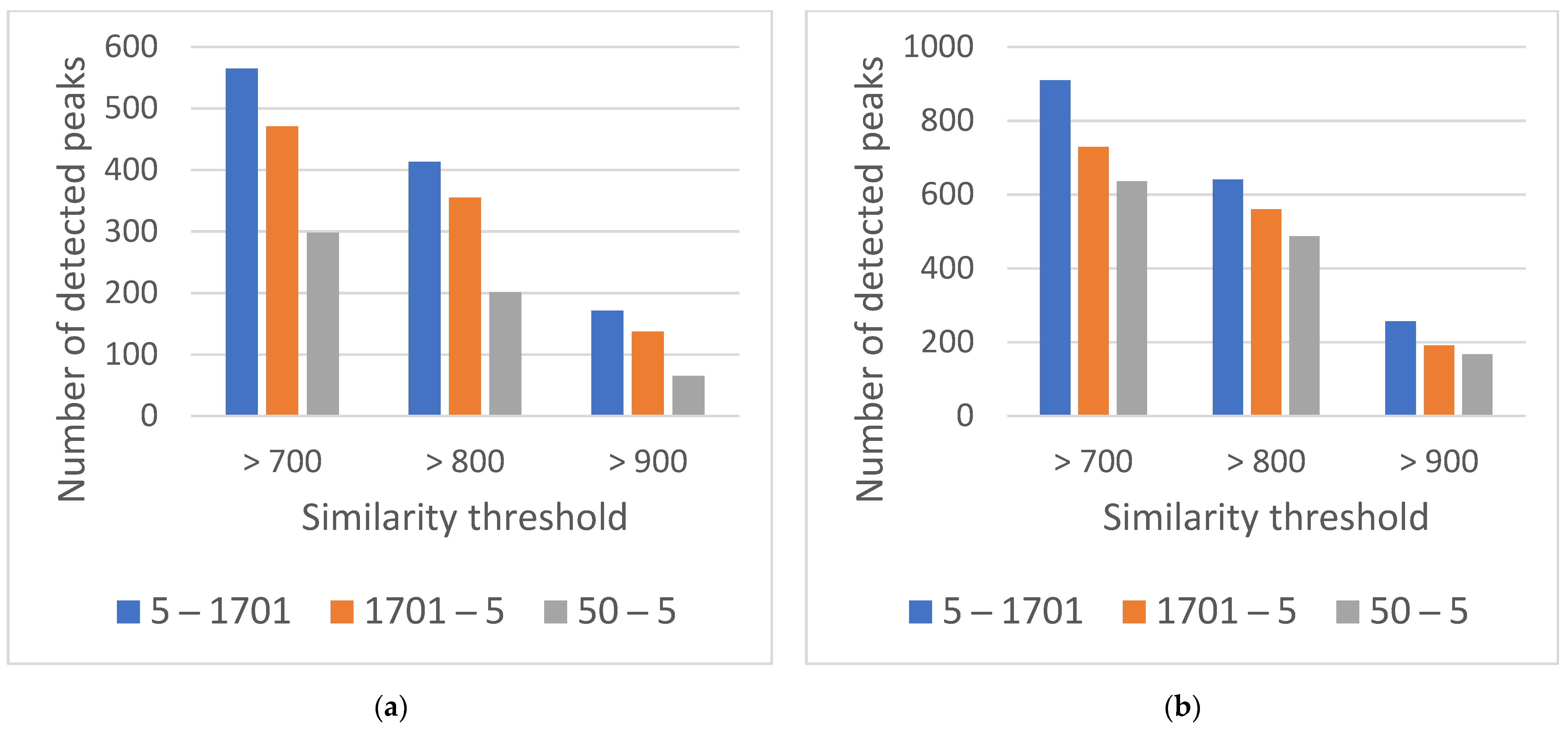
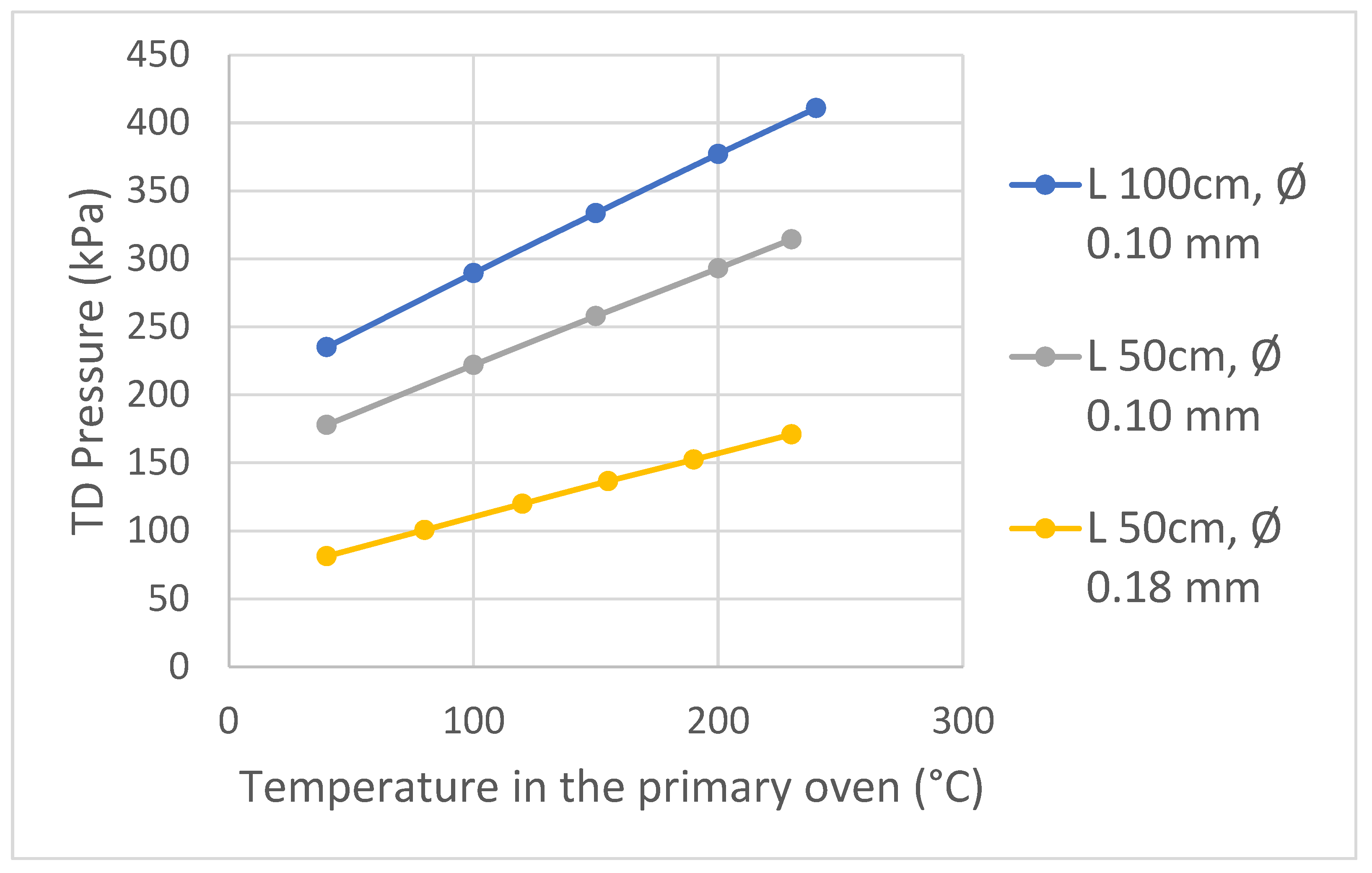
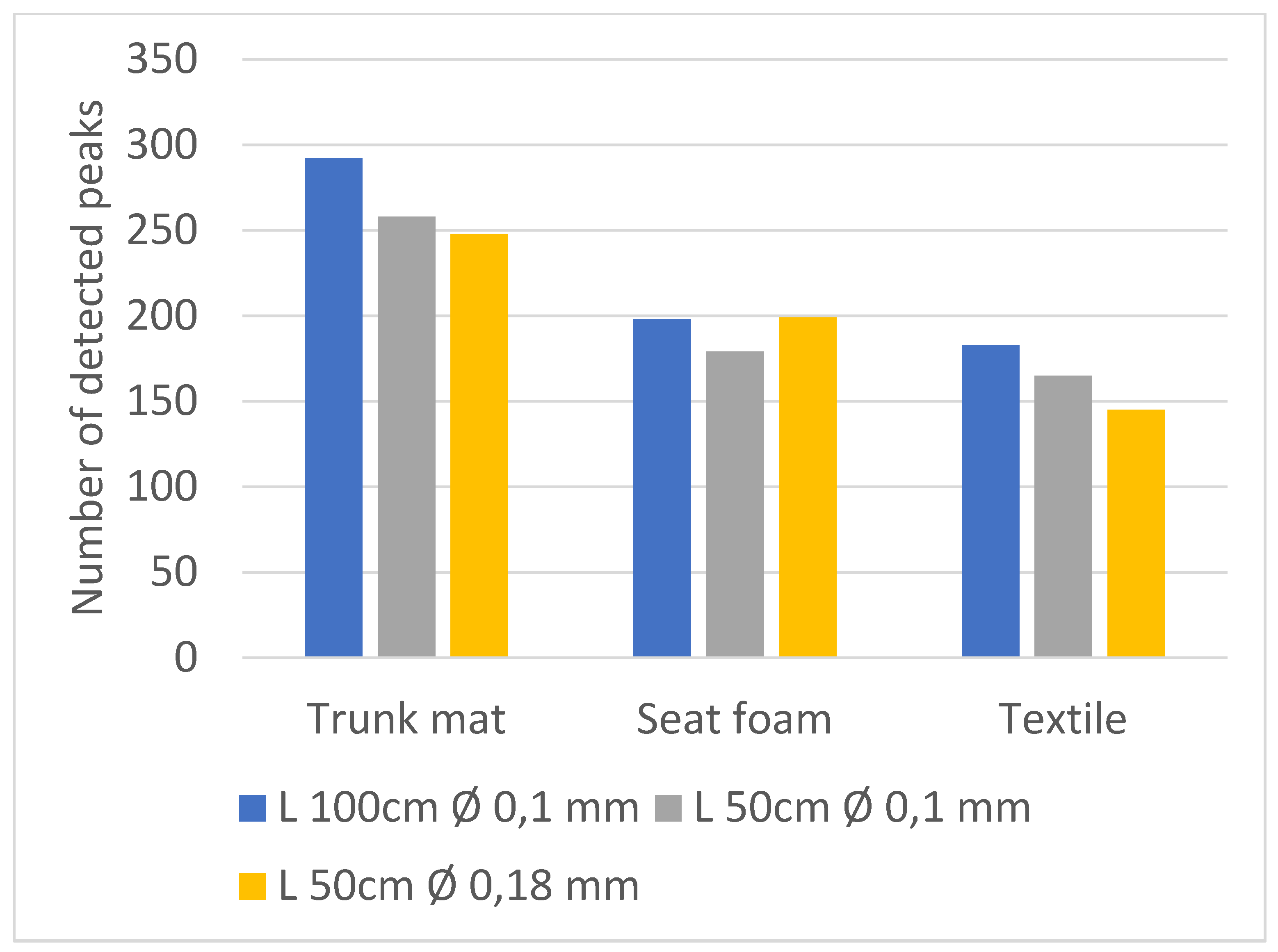
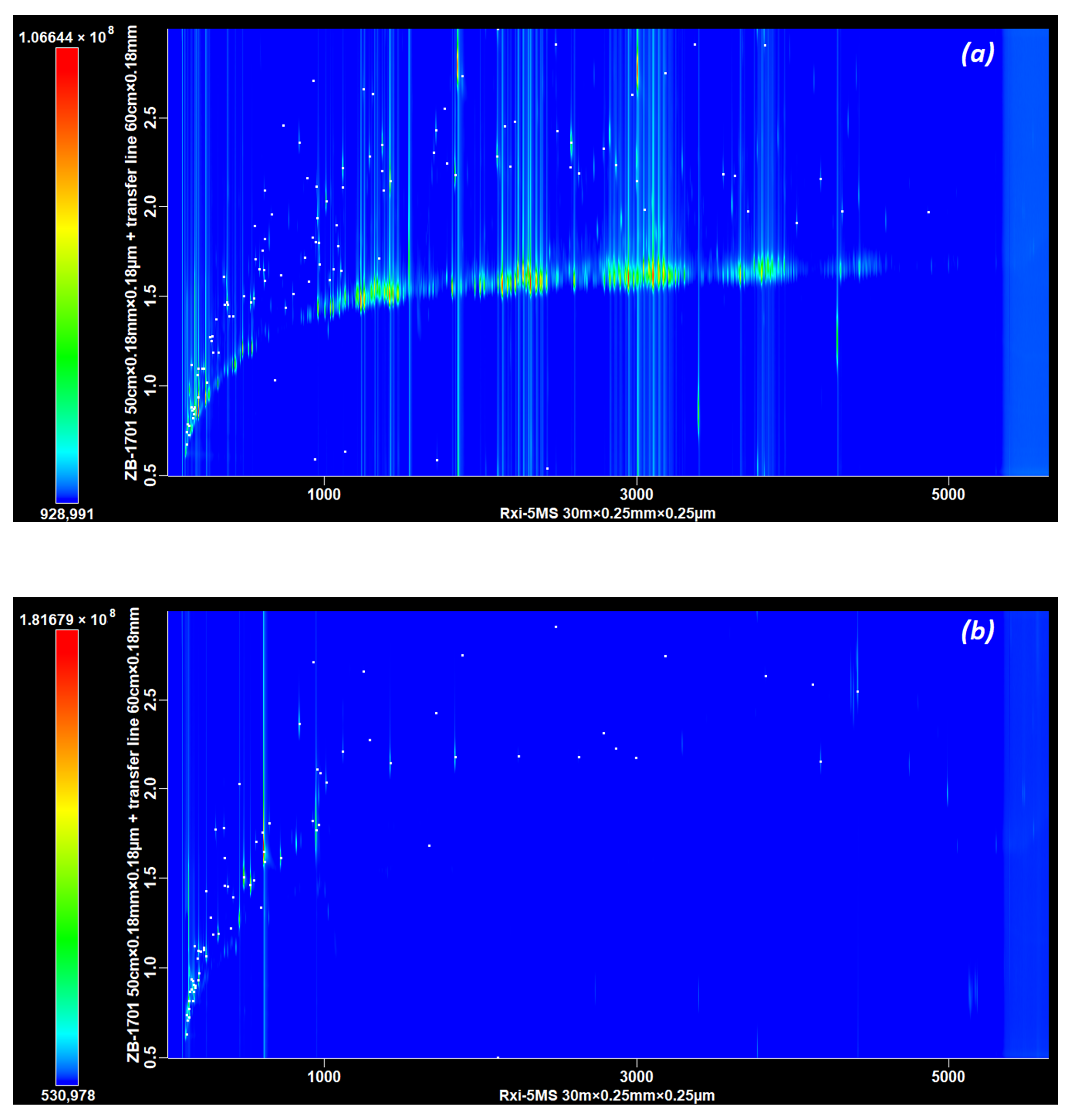
3.2. Part B, Selecting the Dimensions of the ²D Column

The Influence of the Length and Diameter of the Second Dimension Column

In our instrumental configuration, the thermodesorber bypassed and assumed the role of the injector. Therefore, it had to withstand heavy pressure, because it was connected to two columns in series, for an extended time. During the experiments described in Part A, the pressures at the inlet of the TD were generally around 207 kPa/30 psi at rest (40 °C in the primary oven) and 414 kPa/60 psi at the end of the temperature program (220 °C). According to the thermodesorber’s manufacturer, this device must not operate above 60 psi, a respected condition that was adhered to. However, working regularly at such pressures increased the maintenance frequency and may prove to be detrimental for the TD in the long term. A pressure of 138 kPa/20 psi at rest seemed a safer limit, and any further decrease would benefit the device.

In GC × GC, the secondary column bears the largest part of a pressure drop. For example, a 50 cm column with an internal diameter of 0.1 mm is equivalent to a 20 m column with an internal diameter of 0.25 mm [35]. Therefore, based on the protocol of Part A and the selected column configuration (5–1701), it was decided to study the effects of the secondary column diameter and length on global pressure in order to preserve the thermodesorber. At the same time, the quality of separation already achieved needed to be maintained, a factor that was evaluated by the same means as in Part A, i.e., according to the number of potential odorants observed.

Thus, four configurations for the secondary column were studied: two lengths, 50 and 100 cm, and two combinations of diameters and stationary phase thicknesses, 0.1 × 0.1 and 0.18 × 0.18 mm × µm, to maintain constant the phase ratio of β = 500. After the second column, as a 60 cm transfer line with a matching diameter was added before the mass spectrometer, the length of the secondary column had to be shortened compared to that in Part A. Out of these four configurations, the 100 cm long and 0.18 mm wide one presented abnormally high pressure (ranging from 210 to 363 kPa) and poor separation overall. These two elements point out a probable issue with the column or its installation. Unfortunately, it was not possible to redo the experiments due to the limited number of samples; this configuration was not included in the following results.

The effect of ²D configurations on pressure is presented in Figure 2. Only the 50 cm long and 0.18 mm wide column achieved a safety threshold of 138 kPa/20 psi at rest. It illustrated experimentally the much larger impact on the pressure drop of the secondary column in comparison to the primary one in bidimensional gas chromatography, despite its much smaller length.

Following the same logical process as in Part A, the performances of the three column configurations were compared for three materials in terms of the number of peaks observed: a trunk mat (multi-layer wood and felt), a PU foam, and a textile. The results are presented in Figure 3. Similarly to Figure 1, the three chosen thresholds share similar behaviours; therefore, only the threshold of 800 is represented here.

Of the three configurations, the 100 cm long and 0.1 mm wide one (the closest to the Part A protocol) permitted us to observe the greatest number of peaks, with 224 on average. This result is consistent with the fact that thin-film and small-diameter columns provide high efficiency at high gas velocity, thus limiting the loss of performance [36]. However, the 50 cm long and 0.18 mm wide column performed decently, with 197 peaks observed on average.

This loss of performance, amounting to 12% in terms of the average number of observed peaks in comparison to the best column, can be considered acceptable in regard to the benefit for the chromatographic system in the long term. Therefore, the shortest and widest secondary column was eventually selected. This completed the TD-GC × GC-TOFMS hardware hyphenation.

In the end, the protocol developed in this part was considered to have been validated for the study of car material emissions. Its application to another sample of polypropylene allowed for the observation of 858 peaks, including hydrocarbons, out of which 144 were considered potentially odorous molecules, and 113 were reported to be odorous (Figure 4a). With such a large number of odorants, it may prove difficult to explain global odour with only a few of them. Moreover, these odorous molecules were widespread on the chromatogram, and it was not possible to restrict them to a few families or a small contour plot. In this chromatogram, the apparent tailing in the ²D dimension is due to imperfectly modulated concentrated hydrocarbons and the choice of high contrast for the colour plot. This had a very limited impact on peak detection and identification.

The same protocol was also applied to three other materials (one ABS, one decor, and one dashboard, chromatograms in Figure 4b–d) for the search of odorous molecules. This was achieved by comparing the potential odorants retained to chemical databases, primarily Pubchem and The Good Scents Company. Including the aforementioned PP, between 75 and 147 odorous molecules were confirmed to be emitted by these four materials. The 20 most abundant molecules (based on the peak area on the chromatogram) for each material are presented in

Table 2. Lists of the 20 most abundant (based on peak area) odorous molecules detected in the emissions of (a) PP, (b) ABS, (c) dashboard, and (d) décor.

(a) PP
Name	CAS Number	Area	1D Retention Time (s)	2D Retention Time (s)
Tetrahydrofuran	109-99-9	5.31 × 108	169.989	0.884
Diphenyl ether	101-84-8	3.89 × 108	2577.336	2.362
Benzoic acid, methyl ester	93-58-3	3.04 × 108	1369.914	2.351
Nonanal	124-19-6	2.06 × 108	1419.912	2.145
Ethylbenzene	100-41-4	1.96 × 108	527.466	1.468
1-Butanol	71-36-3	1.94 × 108	194.9874	1.099
acetone	67-64-1	1.92 × 108	124.992	0.79
Benzene	71-43-2	1.83 × 108	194.9874	0.939
Naphthalene	91-20-3	1.71 × 108	1712.388	2.43
3-Penten-2-one, 4-methyl-	141-79-7	1.56 × 108	377.4756	1.471
1-Hexanol, 2-ethyl-	104-76-7	1.54 × 108	1117.428	2.218
p-Xylene	106-42-3	1.54 × 108	549.9648	1.49
1-Decanol	112-30-1	1.50 × 108	2104.866	2.283
Decanal	112-31-2	1.42 × 108	1834.884	2.179
Pyridine, 2,4,6-trimethyl-	108-75-8	1.33 × 108	954.936	1.942
Acetic acid	64-19-7	9.30 × 107	147.4908	1.119
1-Dodecanol	112-53-8	7.23 × 107	2864.814	2.237
Phenol	108-95-2	7.17 × 107	944.94	1.804
Benzaldehyde, 3,4-dimethyl-	5973-71-7	7.16 × 107	1882.38	2.691
Furan, 2,3-dihydro-	1191-99-7	6.91 × 107	147.4908	0.801
(b) ABS
Name	CAS Number	Area	1D Retention Time (s)	2D Retention Time (s)
Styrene	100-42-5	2.83 × 109	612.462	1.652
Phenol	108-95-2	2.29 × 109	947.442	1.768
2-Propenenitrile	107-13-1	1.89 × 109	132.4914	0.821
Benzene, chloro-	108-90-7	1.47 × 109	482.469	1.509
Ethylbenzene	100-41-4	9.96 × 108	524.9664	1.464
Methyl methacrylate	80-62-6	6.08 × 108	242.4846	1.069
Benzene, (1-methylethyl)-	98-82-8	4.32 × 108	719.952	1.614
Toluene	108-88-3	3.92 × 108	319.9794	1.193
Ethyl Acetate	141-78-6	3.68 × 108	162.4896	0.871
1-Butanol	71-36-3	2.84 × 108	194.9874	1.101
Propanenitrile	107-12-0	2.50 × 108	147.4908	0.941
Benzaldehyde	100-52-7	2.47 × 108	837.444	2.366
Benzene	71-43-2	1.79 × 108	194.9874	0.936
Carbon disulfide	75-15-0	1.71 × 108	134.9916	0.731
2-butanone	78-93-3	1.65 × 108	154.9902	0.888
Pyrrole	109-97-7	1.44 × 108	302.4804	1.773
Methane, dichloro-	75-09-2	1.10 × 108	132.4914	0.776
Nonanal	124-19-6	8.88 × 107	1419.912	2.146
Formic acid	64-18-6	8.02 × 107	119.9922	0.741
Acetic acid	64-19-7	7.79 × 107	167.4894	1.125
(c) Dashboard
Name	CAS Number	Area	1D Retention Time (s)	2D Retention Time (s)
Pyridine	110-86-1	2.01 × 108	284.982	1.351
Furfural	98-01-1	1.39 × 108	454.971	2.009
Acetic acid	64-19-7	1.21 × 108	149.9904	1.604
Nonanal	124-19-6	1.16 × 108	1419.912	2.146
Decanal	112-31-2	8.78 × 107	1834.884	2.182
Dodecanoic acid	143-07-7	8.49 × 107	3184.794	2.738
Octanoic acid	124-07-2	7.95 × 107	1744,89	2.991
Nonanoic acid	112-05-0	7.93 × 107	2117.364	2.956
Sulphur dioxide	7446-09-5	6.95 × 107	494.9682	0.61
Decanoic acid	334-48-5	6.89 × 107	2484.84	2.904
1-Hexanol, 2-ethyl-	104-76-7	5.61 × 107	1117.428	2.209
Formic acid	64-18-6	5.13 × 107	117.4926	0.744
Hexanal	66-25-1	4.76 × 107	379.9758	1.453
2-Tridecanone	593-08-8	4.52 × 107	2944.812	2.201
Furan, 2,5-dimethyl-	625-86-5	4.15 × 107	242.4846	1.021
1-Dodecanol	112-53-8	3.72 × 107	2867.316	2.228
2(5H)-Furanone	497-23-4	3.48 × 107	744.954	0.959
Benzaldehyde	100-52-7	3.04 × 107	839.946	2.36
Carbon disulfide	75-15-0	2.99 × 107	134.9916	0.72
Heptanal	111-71-7	2.80 × 107	647.46	1.806
(d) Decor
Name	CAS Number	Area	1D retention Time (s)	2D Retention Time (s)
1-Methoxy-2-propyl acetate	108-65-6	6.14 × 109	562.464	1.772
Styrene	100-42-5	3.27 × 109	612.462	1.651
Acetic acid, butyl ester	123-86-4	2.81 × 109	412.4736	1.409
2-Propanol, 1-methoxy-	107-98-2	2.66 × 109	212.4864	1.08
Isobutyl acetate	110-19-0	2.43 × 109	332.4786	1.273
Ethyl Acetate	141-78-6	1.80 × 109	164.9892	0.879
Benzene, 1,2,4-trimethyl-	95-63-6	1.38 × 109	964.938	1.812
p-Xylene	106-42-3	1.19 × 109	549.9648	1.494
Triethylamine	121-44-8	1.16 × 109	217.4862	0.915
Toluene	108-88-3	1.08 × 109	319.9794	1.186
Acetic acid	64-19-7	1.08 × 109	149.9904	1.107
2-Propenenitrile	107-13-1	1.06 × 109	129.9918	0.826
o-Xylene	95-47-6	8.42 × 108	617.46	1.583
Ethylbenzene	100-41-4	8.21 × 108	527.466	1.461
Mesitylene	108-67-8	6.09 × 108	874.944	1.713
Nonanal	124-19-6	5.89 × 108	1419.912	2.149
1-Hexanol, 2-ethyl-	104-76-7	4.74 × 108	1117.428	2.206
α-Methylstyrene	98-83-9	3.93 × 108	924.942	1.827
Benzene, 1,2,3-trimethyl-	526-73-8	3.74 × 108	1074.93	1.892
Ethanol, 2-butoxy-	111-76-2	2.95 × 108	659.958	1.946

. As the exhaustive identification of odorants is very time-consuming, it was conducted on very limited samples, none of them being studied during Part A or Part B.

These last results are a preliminary proof of concept of the variety of molecules the method developed allow us to observe. During our experiments, we observed that the response factor between different molecules may vary more than an order of magnitude, which may alter their relative abundance. Moreover, peaks with an area above 1 × 10⁹ may saturate the detector. Thus, without individual calibration curves, these areas must be considered as indicative. According to the areas measured during system suitability tests with a mixture containing 1 to 10 ng of 48 molecules, the individual compound amount was estimated ranging from 10 to 1000 ng.

4. Conclusions

In this study, we described the successful hyphenation between a Markes TD100-xr thermodesorber and a LECO Pegasus BT4D GC × GC-TOFMS device. Their combination is a first, and proper communication between the two instruments was not trivial and required some tricks. Moreover, without optimisation, our instrumental configuration resulted in the subjection of the thermodesorber to high pressures, close to its recommended limit. The first experimental protocol achieved was adapted by shortening and enlarging the ²D column in order to reduce the global pressure drop. According to our global objective of mapping the potential odorants observed in vehicle material emissions, a special criterion was established to rate the separation performance. It consisted of enumerating the number of non-aliphatic hydrocarbon peaks, associated with their quality, which was assessed using their similarity score in mass spectrometry. An acceptable balance had to be found between the performances in terms of the number of compounds detected and the sustainability of the system, with a pressure that had more than halved at the cost of 12% fewer observed peaks.

The two main parameters selected for the final protocol were the phase combination of the two columns (5%-diphenyl and 14%-cyanopropylphenyl) and the dimensions of the ²D column (50 cm × 0.18 mm × 0.18 µm). This experimental approach allowed us to observe several hundreds of polar potentially odorous molecules while keeping the pressure at rest below 100 kPa.

These results lay the foundation for further experiments on the observed molecules, starting with broader screening and the construction of a comprehensive odorant database. As every step of this study involved the selection of representative vehicle materials, our protocol should be suitable for any material used in this field, maybe even for synthetic materials of other origins, but this prospect remains to be confirmed by considering a wider range of other materials, including recycled ones. For further study, we expect to confront the global observed odorants with the olfactory perception of humans.

References

1. Brancher, M.; Griffiths, K.D.; Franco, D.; De Melo Lisboa, H. A review of odour impact criteria in selected countries around the world. Chemosphere 2017, 168, 1531–1570. [Google Scholar] [CrossRef] [PubMed]
2. Zhang, G.-S.; Li, T.-T.; Luo, M.; Liu, J.-F.; Liu, Z.-R.; Bai, Y.-H. Air pollution in the microenvironment of parked new cars. J. Affect. Disord. 2008, 43, 315–319. [Google Scholar] [CrossRef]
3. Faber, J.; Brodzik, K.; Gołda-Kopek, A.; Łomankiewicz, D. Benzene, toluene and xylenes levels in new and used vehicles of the same model. J. Environ. Sci. 2013, 25, 2324–2330. [Google Scholar] [CrossRef] [PubMed]
4. Brodzik, K.; Faber, J.; Łomankiewicz, D.; Gołda-Kopek, A. In-vehicle VOCs composition of unconditioned, newly produced cars. J. Environ. Sci. 2014, 26, 1052–1061. [Google Scholar] [CrossRef] [PubMed]
5. Yoshida, T.; Matsunaga, I. A case study on identification of airborne organic compounds and time courses of their concentrations in the cabin of a new car for private use. Environ. Int. 2006, 32, 58–79. [Google Scholar] [CrossRef] [PubMed]
6. Yoshida, T.; Matsunaga, I.; Tomioka, K.; Kumagai, S. Interior Air Pollution in Automotive Cabins by Volatile Organic Compounds Diffusing from Interior Materials: I. Survey of 101 Types of Japanese Domestically Produced Cars for Private Use. Indoor Built Environ. 2006, 15, 425–444. [Google Scholar] [CrossRef]
7. Yoshida, T.; Matsunaga, I.; Tomioka, K.; Kumagai, S. Interior Air Pollution in Automotive Cabins by Volatile Organic Compounds Diffusing from Interior Materials: II. Influence of Manufacturer, Specifications and Usage Status on Air Pollution, and Estimation of Air Pollution Levels in Initial Phases of Delivery as a New Car. Indoor Built Environ. 2006, 15, 445–462. [Google Scholar] [CrossRef]
8. Janicka, A.B.; Reksa, M.; Sobianowska-Turek, A. The impact of car vehicle class on volatile organic compounds (VOC’s) concentration in microatmosphere of car cabin. J. KONES 2010, 17, 207–212. [Google Scholar]
9. Chen, X.; Feng, L.; Luo, H.; Cheng, H. Analyses on influencing factors of airborne VOCS pollution in taxi cabins. Environ. Sci. Pollut. Res. 2014, 21, 12868–12882. [Google Scholar] [CrossRef]
10. Xu, B.; Chen, X.; Xiong, J. Air quality inside motor vehicles’ cabins: A review. Indoor Built Environ. 2016, 27, 452–465. [Google Scholar] [CrossRef]
11. Buchecker, F.; Loos, H.M.; Buettner, A. Investigations on the impact of hardening on the odour of an aqueous cavity preservation for automotive applications using sensory and instrumental analysis. Talanta Open 2022, 5, 100095. [Google Scholar] [CrossRef]
12. VDA 276-3 (05/2022), VDA Webshop. Available online: https://webshop.vda.de/VDA/vda-276-3-052022 (accessed on 6 December 2022).
13. ISO 12219-1:2021; Interior Air of Road Vehicles—Part 1: Whole Vehicle Test Chamber—Specification and Method for the Determination of Volatile Organic Compounds in Cabin Interiors. ISO: Geneva, Switzerland. Available online: https://www.iso.org/standard/72410.html (accessed on 15 May 2022).
14. Buchecker, F.; Baum, A.; Loos, H.M.; Buettner, A. Follow your nose—Traveling the world of odorants in new cars. Indoor Air 2022, 32, e13014. [Google Scholar] [CrossRef]
15. Boyle, J.A.; Djordjevic, J.; Olsson, M.J.; Lundström, J.N.; Jones-Gotman, M. The Human Brain Distinguishes between Single Odorants and Binary Mixtures. Cereb. Cortex 2008, 19, 66–71. [Google Scholar] [CrossRef]
16. Laing, D.G.; Eddy, A.; Best, D.J. Perceptual characteristics of binary, trinary, and quaternary odor mixtures consisting of unpleasant constituents. Physiol. Behav. 1994, 56, 81–93. [Google Scholar] [CrossRef] [PubMed]
17. Jaubert, J.-N.; Gordon, G.; Dore, J.-C. Une organisation du champ des odeurs. I: Recherche de critères objectifs. Parfums Cosmét. Arômes 1987, 77, 53–56. [Google Scholar]
18. Jaubert, J.-N.; Gordon, G.; Dore, J.-C. Une organisation du champ des odeurs. II: Modèle descriptif de l’organisation de l’espace odorant. Parfums Cosmét. Arômes 1987, 71–82. [Google Scholar]
19. Verriele, M.; Plaisance, H.; Vandenbilcke, V.; Locoge, N.; Jaubert, J.N.; Meunier, G. Odor evaluation and discrimination of car cabin and its components: Application of the “field of odors” approach in a sensory descriptive analysis. J. Sens. Stud. 2012, 27, 102–110. [Google Scholar] [CrossRef]
20. Agapakis, C.M.; Tolaas, S. Smelling in multiple dimensions. Curr. Opin. Chem. Biol. 2012, 16, 569–575. [Google Scholar] [CrossRef] [PubMed]
21. Kaeppler, K.; Mueller, F. Odor Classification: A Review of Factors Influencing Perception-Based Odor Arrangements. Chem. Senses 2013, 38, 189–209. [Google Scholar] [CrossRef]
22. Brattoli, M.; Cisternino, E.; Dambruoso, P.R.; De Gennaro, G.; Giungato, P.; Mazzone, A.; Palmisani, J.; Tutino, M. Gas Chromatography Analysis with Olfactometric Detection (GC-O) as a Useful Methodology for Chemical Characterization of Odorous Compounds. Sensors 2013, 13, 16759–16800. [Google Scholar] [CrossRef]
23. Delahunty, C.M.; Eyres, G.; Dufour, J.-P. Gas chromatography-olfactometry. J. Sep. Sci. 2006, 29, 2107–2125. [Google Scholar] [CrossRef] [PubMed]
24. Giungato, P.; Di Gilio, A.; Palmisani, J.; Marzocca, A.; Mazzone, A.; Brattoli, M.; Giua, R.; de Gennaro, G. Synergistic approaches for odor active compounds monitoring and identification: State of the art, integration, limits and potentialities of analytical and sensorial techniques. TrAC Trends Anal. Chem. 2018, 107, 116–129. [Google Scholar] [CrossRef]
25. Mondello, L.; Tranchida, P.Q.; Dugo, P.; Dugo, G. Comprehensive two-dimensional gas chromatography-mass spectrometry: A review. Mass Spectrom. Rev. 2008, 27, 101–124. [Google Scholar] [CrossRef] [PubMed]
26. Murray, J.A. Qualitative and quantitative approaches in comprehensive two-dimensional gas chromatography. J. Chromatogr. A 2012, 1261, 58–68. [Google Scholar] [CrossRef]
27. Lee, A.L.; Bartle, K.D.; Lewis, A.C. A Model of Peak Amplitude Enhancement in Orthogonal Two-Dimensional Gas Chromatography. Anal. Chem. 2001, 73, 1330–1335. [Google Scholar] [CrossRef]
28. Czerny, M.; Brueckner, R.; Kirchhoff, E.; Schmitt, R.; Buettner, A. The Influence of Molecular Structure on Odor Qualities and Odor Detection Thresholds of Volatile Alkylated Phenols. Chem. Senses 2011, 36, 539–553. [Google Scholar] [CrossRef]
29. Chastrette, M. Data Management in Olfaction Studies. SAR QSAR Environ. Res. 1998, 8, 157–181. [Google Scholar] [CrossRef] [PubMed]
30. Blomberg, J.; Schoenmakers, P.J.; Beens, J.; Tijssen, R. Compehensive two-dimensional gas chromatography (GC × GC) and its applicability to the characterization of complex (petrochemical) mixtures. J. High Resolut. Chromatogr. 1997, 20, 539–544. [Google Scholar] [CrossRef]
31. Ochiai, N.; Sasamoto, K. Selectable one-dimensional or two-dimensional gas chromatography–olfactometry/mass spectrometry with preparative fraction collection for analysis of ultra-trace amounts of odor compounds. J. Chromatogr. A 2010, 1218, 3180–3185. [Google Scholar] [CrossRef]
32. ISO 12219-3:2012; Interior Air of Road Vehicles—Part 3: Screening Method for the Determination of the Emissions of Volatile Organic Compounds from Vehicle Interior Parts and Materials—Micro-Scale Chamber Method. ISO: Geneva, Switzerland. Available online: http://www.iso.org/cms/render/live/en/sites/isoorg/contents/data/standard/05/48/54866.html (accessed on 30 August 2019).
33. Jores, C.D.S.; Klein, R.; Legendre, A.; Dugay, J.; Thiébaut, D.; Vial, J. Preparation of Thermodesorption Tube Standards: Comparison of Usual Methods Using Accuracy Profile Evaluation. Separations 2022, 9, 226. [Google Scholar] [CrossRef]
34. Wilson, R.B.; Siegler, W.C.; Hoggard, J.C.; Fitz, B.D.; Nadeau, J.S.; Synovec, R.E. Achieving high peak capacity production for gas chromatography and comprehensive two-dimensional gas chromatography by minimizing off-column peak broadening. J. Chromatogr. A 2011, 1218, 3130–3139. [Google Scholar] [CrossRef]
35. Shellie, R.; Marriott, P.; Morrison, P.; Mondello, L. Effects of pressure drop on absolute retention matching in comprehensive two-dimensional gas chromatography. J. Sep. Sci. 2004, 27, 503–512. [Google Scholar] [CrossRef]
36. Mommers, J.; van der Wal, S. Column Selection and Optimization for Comprehensive Two-Dimensional Gas Chromatography: A Review. Crit. Rev. Anal. Chem. 2021, 51, 183–202. [Google Scholar] [CrossRef]
Scheme 1. A simplified scheme of the carrier gas flow in the thermodesorber (a) at rest/during program and (b) during injection. Carrier gas flows are represented in green.
Separations 11 00162 sch001
Figure 1. Number of peaks per similarity threshold for polypropylene (a) and synthetic leather (b).
Separations 11 00162 g001
Figure 2. The influence of the secondary column dimension on the TD pressure.
Separations 11 00162 g002
Figure 3. Number of potential odorants detected at similarity threshold of 800 depending on second column dimensions.
Separations 11 00162 g003
Figure 4. Chromatograms of 4 materials with the validated protocol: (a) PP, (b) ABS, (c) dashboard, and (d) décor. x axis: 1D retention time (s). y axis: 2D retention time (s). Each white square represents one of the identified odorant (75 in dashboard and ABS, 113 in PP, and 143 in dashboard).
Separations 11 00162 g004aSeparations 11 00162 g004b