Review

A Review of Prediction and Optimization for Sequence-Driven Scheduling in Job Shop Flexible Manufacturing Systems

by
Prita Meilanitasari
1 and
Seung-Jun Shin
2,*
1
Graduate School of Technology and Innovation Management, Hanyang University, Seoul 04763, Korea
2
Division of Interdisciplinary Industrial Studies, Hanyang University, Seoul 04763, Korea
*
Author to whom correspondence should be addressed.
Processes 2021, 9(8), 1391; https://doi.org/10.3390/pr9081391
Submission received: 16 July 2021 / Revised: 2 August 2021 / Accepted: 5 August 2021 / Published: 11 August 2021
(This article belongs to the Special Issue Modeling, Simulation and Control of Flexible Manufacturing Systems)

Abstract

:
This article reviews the state of the art of prediction and optimization for sequence-driven scheduling in job shop flexible manufacturing systems (JS-FMSs). The objectives of the article are to (1) analyze the literature related to algorithms for sequencing and scheduling, considering domain, method, objective, sequence type, and uncertainty; and to (2) examine current challenges and future directions to promote the feasibility and usability of the relevant research. Current challenges are summarized as follows: less consideration of uncertainty factors causes a gap between the reality and the derived schedules; the use of stationary dispatching rules is limited to reflect the dynamics and flexibility; production-level scheduling is restricted to increase responsiveness owing to product-level uncertainty; and optimization is more focused, while prediction is used mostly for verification and validation, although prediction-then-optimization is the standard stream in data analytics. In future research, the degree of uncertainty should be quantified and modeled explicitly; both holistic and granular algorithms should be considered; product sequences should be incorporated; and sequence learning should be applied to implement the prediction-then-optimization stream. This would enable us to derive data-learned prediction and optimization models that output accurate and precise schedules; foresee individual product locations; and respond rapidly to dynamic and frequent changes in JS-FMSs.

1. Introduction

Flexible manufacturing systems (FMSs) are manufacturing systems that can fabricate diverse product types simultaneously under programmed control at various workstations [1]. FMSs consist of a group of workstations that are interconnected through automated material handling systems and storage systems, and controlled by a computer-integrated system [2]. Along with the advancement of not only manufacturing technology, but also information and communication technology (ICT), FMSs have evolved to handle more diverse product types with greater efficiency and effectiveness. A multimodal factory is a representative example of a modern FMS, which can fabricate and assemble various products demanded across heterogeneous industrial sectors in a single facility [3].
Earlier FMSs were complex, heavy, and poorly adaptive; meanwhile, recent FMSs have become simpler, lightweight, and highly adaptive. The trend in FMS development is advancing toward a smaller version of the traditional FMS, i.e., flexible manufacturing cells (FMCs) [2]. An FMC comprises two or more computerized numerical control (CNC) machines, and produces a variety of products cell-by-cell, thereby making FMSs more agile and flexible. However, uncertainty is a critical issue in FMSs. The increased agility and flexibility of recently developed FMSs has resulted in increased uncertainty. Uncertainty refers to any unpredictable events that disturb manufacturing operations owing to limited machine capacity, diverse setup and processing times, sudden orders, machine failures, deadlocks, cost fluctuations, or demand changes, as well as other, unknown reasons [4]. Uncertainty naturally has negative impacts on targeted performance metrics, such as lead time, due date, production time, inventory, and throughput [2]. Therefore, it is essential to resolve uncertainty issues to increase—or at least, sustain—the targeted performance in FMSs by determining the cause and effect of uncertainty with quantitative and predictable means.
FMSs can be subdivided into open shops, flow shops, and job shops based on job processing orders [5]. Among them, the job shop type is commonly used because it is easy to set up, add, change, or remove resources as needed, with the flexibility to increase the capacity to cope with demand changes [6]. The job shop processes each job on machines within a given processing time, and the machines can process only one operation for each job [7]. Accordingly, job shop flexible manufacturing systems (JS-FMSs) refer to job-shop-style FMSs, where a set of available machines is selected for individual jobs and higher flexibility and complexity are demanded in scheduling [7]. Job flows are dynamic in JS-FMSs; because a job flow can frequently change owing to time-dependent dynamics, information regarding job arrivals and their arrival times is difficult to obtain in advance [8]. In JS-FMSs, the timing of job arrivals is important because it can be used to determine when each job arrives in the designated machine, and it is largely associated with scheduling problems. When the timing of job arrivals is unknown, it is difficult to derive accurate schedules that consider the in situ status. As a result, scheduling problems have mostly relied on assumptions under which jobs arrive randomly or serially, as well as approximations where descriptive statistics such as the mean and deviation are used instead of accurate values for individual jobs [8].
Scheduling refers to the allocation of limited resources over time to perform a given set of jobs [9]. Scheduling involves two types of decisions: (1) allocation decisions—that is, which machines will be assigned to perform the given jobs—and (2) sequencing decisions—that is, which and when jobs will be performed in the designated machines [9]. Production scheduling is generally established based on dispatching rules that include earliest due date (EDD), shortest processing time (SPT), and first-come-first-serve (FCFS) [10]. However, such stationary dispatching rules may cause large discrepancies between schedules and actual results, owing to the dynamics and uncertainty in JS-FMSs. In addition, they rarely trace the exact locations of individual products in (near) real time, because they also rely on assumptions and approximations, as described above. In this regard, prediction is significant for scheduling so that manufacturers can foresee the allocations and sequences of product flows. Schedule prediction allows proactive actions to increase productivity or prepare alternatives to cope with uncertainty. Schedule optimization is also important to determine the best allocations and sequences under constraints, thereby enhancing the target performance. Accordingly, many previous studies have endeavored to develop mathematical and heuristic algorithms for the prediction and optimization of scheduling by considering major uncertainty factors (refer to Section 3). However, most of these studies are biased toward optimization rather than prediction.
Sequencing refers to the order of processing a set of tasks over available resources [8]. Naturally, sequencing involves the determination of the allocations and flows of a set of tasks with regard to resources, products, and jobs. Sequencing is typically complex in JS-FMSs. Uncertainty also forces sequences to be changed and disrupted frequently. Thus, sequencing should be determined prior to scheduling, and it should be adaptively updated whenever changes occur in an actual JS-FMS. Sequences can be divided into three categories, as shown in Figure 1. The resource sequence is related to the macro-level process flow, as determined by resource allocation. The product sequence represents the flows and positions of individual products on a certain resource. This sequence allows the traceability of products. The job sequence refers to the micro-level process flow occurring in each job. The product sequence needs to be considered as an important viewpoint, because schedules that necessitate the calculation of time-domain performances can be feasibly created after the product sequence has been identified preferentially.
The scheduling and sequencing of an FMS is a traditional problem. Accordingly, review papers have provided remarkable analyses of the relevant literature. However, we discovered certain limitations in existing review papers, as detailed in Section 2.1. Existing reviews are confined to optimization problems based on methods and objective functions; moreover, they rarely incorporate uncertainty issues, and they limit the importance of sequencing, particularly at the product level.
This article presents a review of prediction and optimization for sequence-driven scheduling in JS-FMSs. The objectives of this study are to (1) provide analytical information concerning the state of the art of schedule prediction and optimization; (2) offer insight into the causality between sequencing and scheduling; and (3) discuss challenges and future research directions to promote the accuracy and robustness of schedule prediction and optimization. In particular, this article introduces sequence learning, which is a branch of machine learning that involves sequence prediction, generation, recognition, and decision. This article proposes that a sequence-learning-based approach can be leveraged to create data-driven models from learning data to adaptively incorporate the dynamics and uncertainty in JS-FMSs.
The remainder of this paper is organized as follows: Section 2 explains the scope and methodology of the literature review; Section 3 presents our macro- and micro-level analyses of the literature; Section 4 discusses the challenges and future directions; and Section 5 summarizes our conclusions.

2. Scope and Method

This section explains the scope and methods of our literature analysis. Section 2.1 analyzes previous review papers relevant to scheduling in FMSs; Section 2.2 and Section 2.3 describe the scope and methodology of our literature review, respectively.

2.1. Review of Previous Reviews

FMS scheduling is a typical and traditional problem in the field of manufacturing. Because of this, dozens of review papers have reviewed and analyzed the relevant literature. These reviews have provided meaningful information and findings on FMS scheduling from holistic and in-depth perspectives. Table 1 summarizes the review papers on FMS scheduling; we analyze them in terms of keywords, production type, and their findings. These reviews have contributed to introducing approaches, technologies, methodologies, and systems regarding FMS scheduling to manufacturing and computer engineers, technicians, and scientists. However, the previous review papers exhibit the following limitations:
  • They are confined to optimization problems, with bias toward algorithms and objective functions [7,11,12,13];
  • They rarely accommodate uncertainty issues and their subsidiary factors, such as setup time, buffer size, and transportation time [7,11,14];
  • They are limited in addressing the importance of product allocations and sequences, owing to dependency on stationary dispatching rules [7,14,15].
Table 1. Review papers on scheduling in FMSs.
Author KeywordProduction TypeFindings
Zhu X and Wilhelm (2006) [11]
Scheduling in sequence-dependent setup (SDS)
Optimization
Single machine
Parallel machine
Flow shop
Job shop
Classify lot sizing and sequence-dependent setup (SDS) in flow shop and job shop scheduling.
Suggest a new objective function and new approach with combination of lot sizing and SDS
Demir and İşleyen (2013) [14]
Flexible job shop scheduling problem (FJSP)
Optimization
Flexible job shop
Compare and classify optimization solution models using mathematical formulations in terms of binary variables.
Propose a time-indexed model for FJSP
Chaudhry and Khan (2016) [12]
Flexible job shop scheduling (FJSS)
Flexible job shop
Classify FJSS techniques based on variations in methods using a survey method
Gao et al. (2019) [13]
FJSP
Optimization
Resource sequence
Flexible job shop
Classify literature using swarm intelligence and evolutionary algorithms for solving FJSP
Zhang et al. (2019) [15]
Job shop
Optimization
Prediction
Dynamic job shop
Classify job shop scheduling problem (JSP) in terms of methods and constraints
Build a framework to solve JSP in Industry 4.0.
Xie et al. (2020) [7]
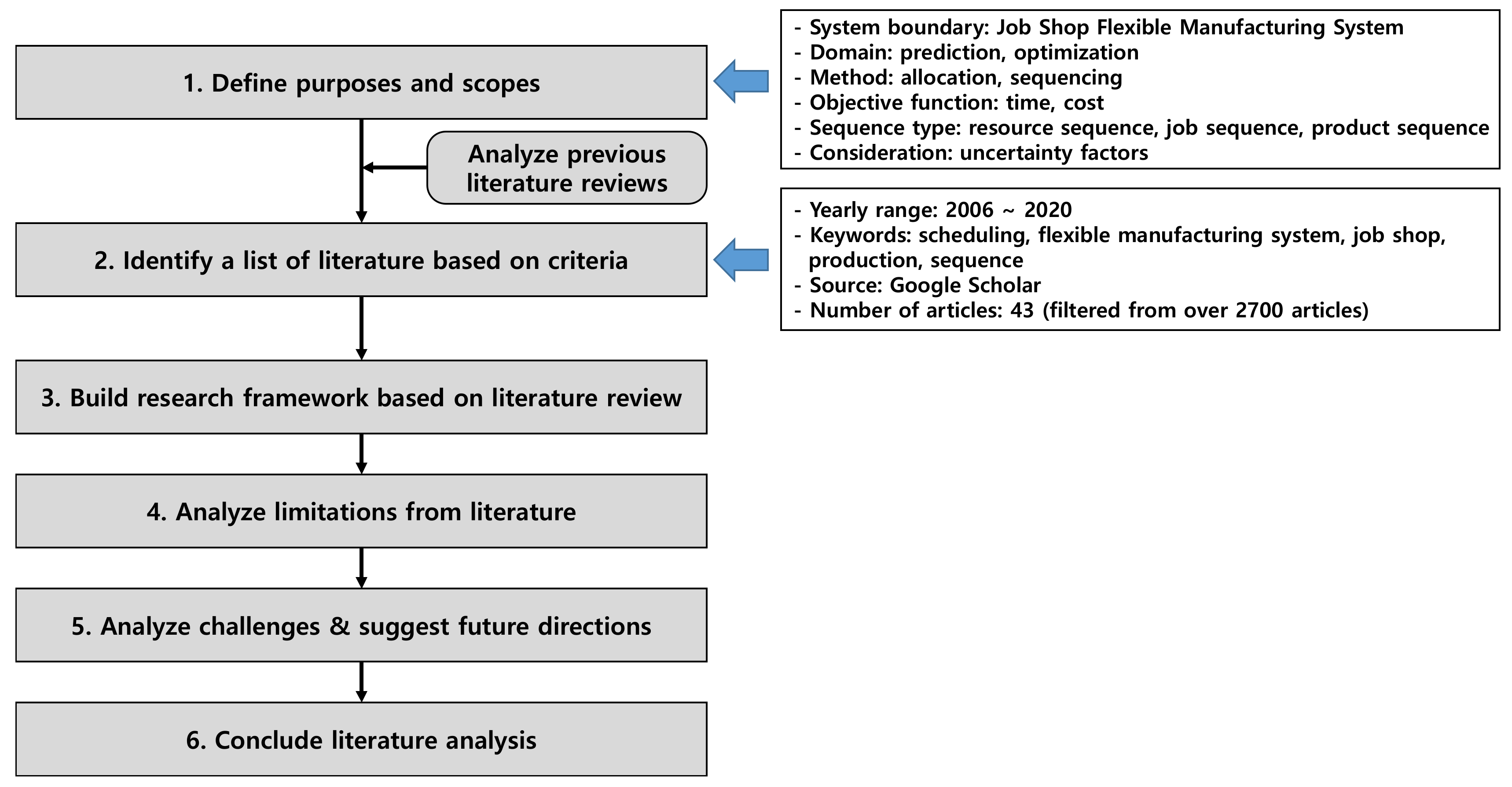
FJSP
Optimization
Total Flexible job shop
Partial Flexible job shop
Classify literature based on mathematical modelling (MILP, LP, etc.); heuristic (hybrid); and metaheuristic (GA, VNS)

2.2. Scope

To provide a different view from the previous review papers, we select “optimization”, “prediction”, “schedule”, “sequence”, and “uncertainty” as primary aspects. We set up the target areas to provide more concise information and insights. The scope of our literature review is as follows:
System boundary: job shop flexible manufacturing systems (JS-FMS);
Domain: prediction and optimization;
Primary method: scheduling and sequencing;
Objective function: time indicators and cost indicators;
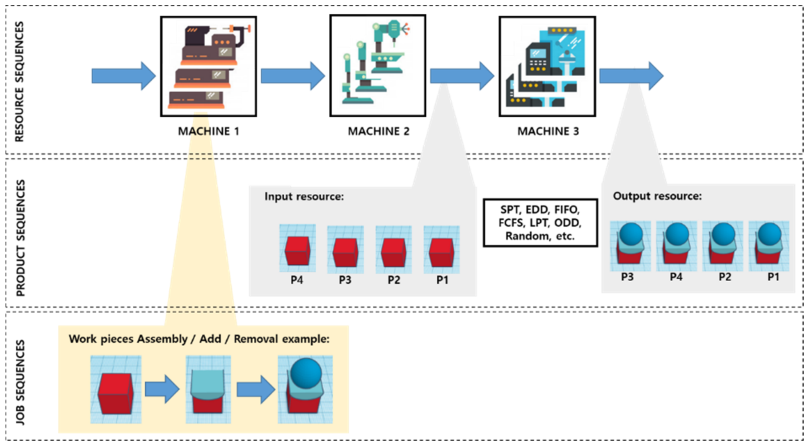
Sequence type: resource sequence, job sequence, and product sequence;
Consideration: uncertainty factors.

2.3. Methodology

Figure 2 illustrates the research methodology; this methodology is revised from Rasheed and Wahid [16], and Akbar and Irohara [17], as they suggest reasonable and logical procedures for literature review and analysis. In the first step, the purpose and scope of the review are defined, as described in Section 2.2. Second, a list of literature within the target areas is identified. Here, we searched for the following keywords using Google Scholar: “scheduling”, “flexible manufacturing system”, “job shop”, “production”, and “sequence”. We obtained over 2700 articles from online journal sources. We then chose the literature filtered by only journals and international proceedings from the past 14 years (2006–2020). The determination of this duration stems from our judgment that the relevant technologies have recently been growing rapidly.
We extracted 47 articles that directly related to the scope of our research from online sources, as presented in Table 2. Third, the research framework is constructed from our in-depth review processes. This step derives classification criteria based on the findings in the literature. Fourth, the limitations of the literature are analyzed. Fifth, the current challenges and future directions are discussed to provide insights. Finally, our literature review is concluded in the sixth step.

3. Literature Analysis

This section describes the analysis of the literature review. Constructing a research framework that classifies and summarizes the research streams derived from the articles of interest would facilitate an effective elucidation. Section 3.1 introduces the research framework and our review summary; Section 3.2 explains the details of our literature review.

3.1. Review Summary

The research framework is illustrated in Figure 3; this framework comprises the layers of domain, method, objective, sequence type, and uncertainty. In Figure 3, we derive items from the individual articles reviewed. Table 3 summarizes the articles in terms of their domain, method, objective, sequence type, and uncertainty.
The domain layer is separated into optimization and prediction. Each article is separated depending on whether it concentrates on optimization to improve the target performance with the best input parameters, or prediction to determine the relationship between the input parameters and the target performance. In our analysis, most of the articles of interest concern optimization. Meanwhile, some articles consider prediction as well as optimization, although they mainly aim at optimizing the target performance, followed by prediction for verification and validation purposes.
The method layer is classified into metaheuristic, mathematical modeling, and machine learning; this classification is based on the major methods used to solve the problem described in each article. Metaheuristic and mathematical modeling methods were used in many of the studies; this is attributed to the fact that these articles addressed optimization problems, wherein metaheuristic and mathematical modeling are commonly used. On the other hand, machine learning has become increasingly popular, as it yields knowledge and insights from historical and training data [18].
The objective layer contains diverse performance indicators that relate to time or cost domain metrics, as well as the objective function that identifies the optimization purpose of the indicators. Productivity is critical in JS-FMSs, as described in Section 1. Many articles have contributed to minimizing production time, wasted time, and production costs by deriving models or solutions optimized for target indicators. Some articles solve multi-objective optimization problems that involve more than two indicators. Meanwhile, others solve single-objective optimization problems. Note that environmentally conscious indicators have recently received attention, owing to the increased importance of environmental issues, even in JS-FMSs; however, these are beyond the scope of this article (refer to [17] for details).
The sequence type layer indicates the sequence types and dispatching rules. Many of the articles apply common dispatching rules (e.g., FIFO, RAND, and SPT) to optimize machine and job sequences; they rely on static dispatching rules, and do not consider the dynamics and changes of such sequences during production. Moreover, the availability of product sequences is not meaningfully incorporated, despite its significant influence on machine and job sequences.
The uncertainty layer involves uncertainty factors including limited machine capacity, diverse processing time, sudden orders, machine failure, deadlock, cost fluctuation, demand change, and unknown reasons. Many of the articles considered setup time and processing time as uncertainty factors. Some articles apply the concept of sequence-dependent setup time (SDST). Here, SDST means that the start time of a job in a machine is determined depending on the finish time of the previous job [19]. A mutual causality between setup time and processing time exists in scheduling and, thus, this complex relationship hinders the accurate anticipation of resource, job, or product sequences. In this regard, uncertainty affects schedules and sequences, and can thus create a large gap between the desired and actual results. However, determining the uncertainty and its associated influences can be ambiguous and difficult, hence the term “uncertainty”.
Table 3. Summary of articles.
NoAuthorsOptimization(O)/
Prediction(P)
TechniquesObjectiveSequenceUncertainty
ResourceJobProductDispatching Rule
1Luo et al. (2008) [20]OACO & LSMS, WL SPTN/A
2Pezzella et al. (2008) [21]OGAMS MWR & MORPT
3Vinod et al. (2008) [22]O & PSIMULATIONMT, MFT, MST, MNS FIFO, SPT, EDD, EMDD, CR, SSPT, SIMSET, JSPT, JEDD, JEMDD, JCR, JSSPTST & PT
4Qiu et al. (2009) [23]OGAMS RANDN/A
5Song et al. (2010) [24]OGA and LSMS RANDN/A
6Wang et al. (2010) [25]OFBSMS, TWL, CMW N/AMA
7Bagheri et.al. (2011) [26]OVNSMS & MT RANDST
8Moslehi et al. (2011) [27]OPSOMS, TWL, KT SPTPT
9Wan et al. (2011) [28]OGAMS RAND, MWR, MORN/A
10Xue et al. (2011) [29]OHDSTC SDST
11Agrawal et al. (2012) [30]O&PGAMS & TMT SDPT
12Gao et al. (2012) [31]O&PPDHSMS & MT SPT, EFTRAND, MWR, MORN/A
13Özgüven et al. (2012) [32]OMIGPMT, MS, WL SDST & PT
14Xiong et al. (2012) [33]O&PGAMS RANDMB
15Xu et al. (2012) [34]ODAMMS N/AComplex Product
16Chen et al. (2013) [35]OWBMRMT FIFO, WSPT, SPRT, RRrule, WBMRN/A
17Kechadi (2013) [36]O & PRNNMS WSPT & WLPTPT
18Yuan et al. (2013) [37]OHHS
(NN & HS)
MS MWRN/A
19Liu et al. (2014) [38]OGAMS RANDN/A
20Song et al. (2014) [39]ODSPMS SDPN/A
21Moghadam et al. (2014) [40]O & PGAMS RANDPT & WL
22Rossi (2014) [41]OSIAMS SDUE
23Abdelmaguid (2015) [42]OTS, NSFMS RAND & MODST & PT
24Palacios et al. (2015) [43]O & PHGA
(GA & TS)
TT & MS N/APT
25Ham et al. (2016) [44]OMIP & CPMS SDN/A
26Torkaman et al. (2017) [45]OMIPIC SDST, Q, PT, NoP
27Gong et al. (2018) [46]O & PHGAMS, TWC, GP(+)* N/AN/A
28Jamrus et al. (2018) [47]OPSO & GACT RANDPT
29Shen et al. (2018) [19]OMILP & TSMS SDST & PT
30Zhang et al. (2018) [48]OMILP & CPMS ECT, JMRW, MLWMB, MU, RO
31Novas (2019) [49]OCPMS SDMC
32Li et al. (2019) [50]OSHMS & TSC RANDST
33Huang et al. (2019) [51]O & PHGA
(GA & SA)
MS SPTTTransfer Time
34Wu et al. (2019) [52]ODDE, SA, CSAMS N/APT
35Zhang et al. (2019) [53]O & PIH-PSO
(PSO, GA, SA)
MS, ML, PC, BML SDST
36Zhao et al. (2019) [54]ODRLMS N/AN/A
37Zhou et al. (2019) [55]O & PMAHHTTO & WT RANDBML & EC
38Abreu et al. (2020) [56]O & PHGA(GA, SA, VNS)MS SDST
39Defersha et al. (2020) [57]OGAMS SDST
40Fattahi et al. (2020) [58]OPSO & PVNSMS RANDN/A
41Gu et al. (2020) [59]OPSOMS, BML, TW RAND & GSOPT
42Lin (2020) [60]OGAMS RANDPT
43Luo (2020) [61]ORLTT FIFO, EDD, MRT, SPT, LPTNew Job Insertion
44Wang et al. (2020) [62]OABCMS RANDPT
45Wu et al. (2020) [63]OCSAMS FIFOPT
46Wu et al. (2021) [64]OBranch and BoundTT N/APT
47Wu et al. (2021) [65]ODDE, IG, GAMS N/APT
* (+): purpose maximization; N/A: information not available.

3.2. Detailed Analysis
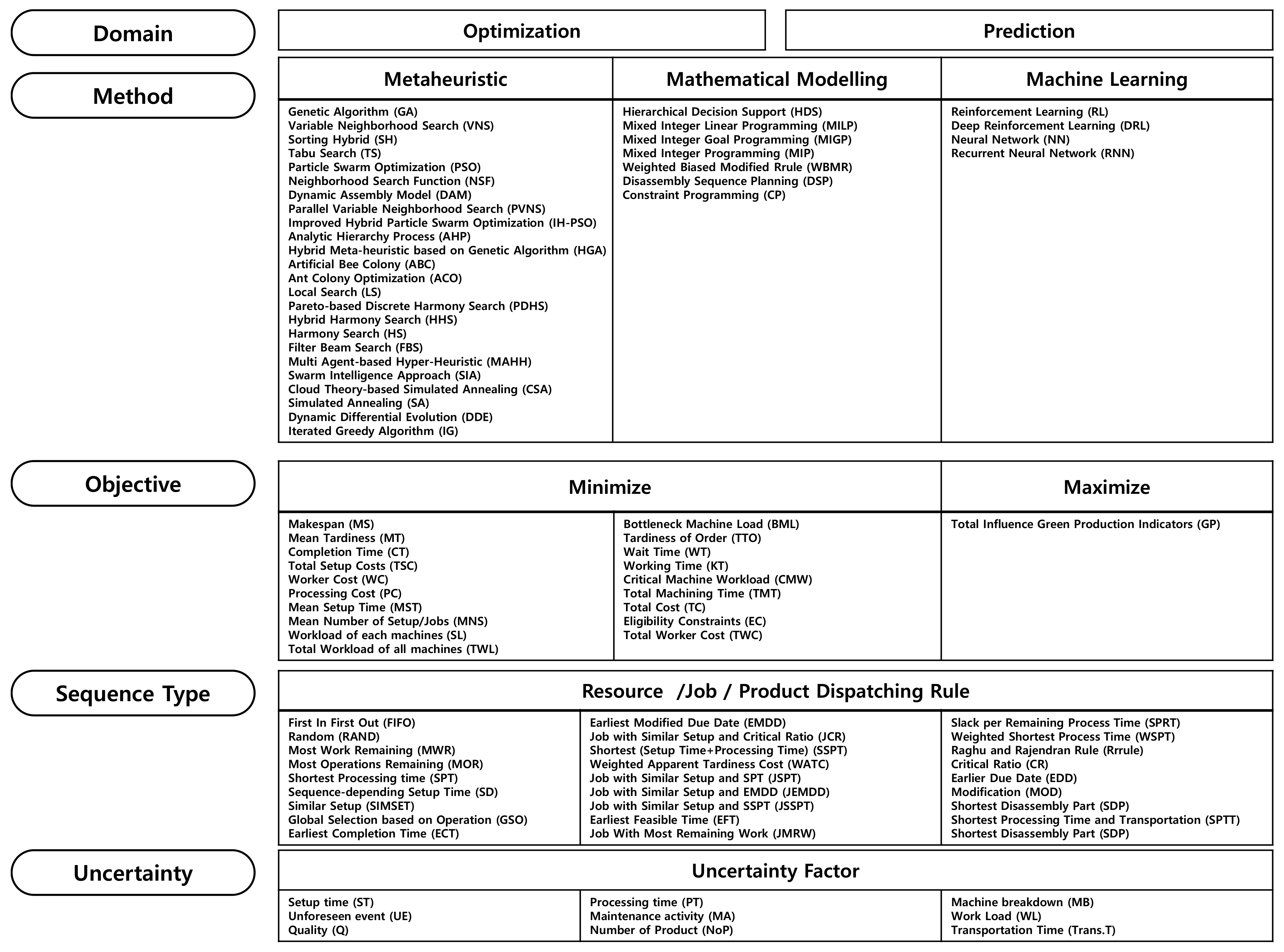
This subsection explains the details of our literature analysis in terms of the domain, method, objective, sequence type, and uncertainty layers.

3.2.1. Domain

Prediction and optimization are challenging. Many real-world analytics problems are always faced with prediction and optimization issues; meanwhile, “predict-then-optimize” is known as the standard stream [46]. However, we find that “optimize-then-predict” is a common stream in the research area of JS-FMSs. This is because optimizing schedules and sequences is the most typical problem in JS-FMSs. Predicting schedules and sequences is generally used to verify and validate the results derived from the optimization algorithms and solutions.
In our analysis, all of the articles are focused on schedule and sequence optimization, as shown in Table 3. Some of them develop optimization algorithms and then carry out predictions to demonstrate whether their algorithms are effective and efficient under given scenarios. In this case, it is difficult to clearly separate optimization and prediction. Vinod et al. [22], Agrawal et al. [30], Zhang et al. [53], Abreu et al. [56], Huang et al. [51], Gao et al. [31], Moghadam et al. [40], Zhou et al. [55], Xiong et al. [33], Palacios et al. [43], Kechadi [36], and Gong et al. [46] combine optimization and prediction. They first develop optimization algorithms and solutions for their desired objectives (e.g., time, cost, and workload). Second, they obtain predictive results or measure predictive performance on resource, product, and job sequences by running their algorithms and solutions. However, they are limited in their ability to accurately predict the positions and allocations of individual products; this is because their algorithms and solutions use theoretical and stationary approaches, which rarely accommodate rapid and frequent changes in JS-FMSs.
In this context, optimization is still important in the research area of JS-FMSs. Furthermore, prediction is also important to accurately anticipate the sequences of resources, jobs, and products, even in complex and dynamic JS-FMS environments. This prediction should be applied not only to verify and validate results, but also to develop algorithms and solutions that respond to real situations. Thus, the standard stream—i.e., “predict-then-optimize”—in the research area of JS-FMSs can be built.

3.2.2. Method

Scheduling in JS-FMSs is well known as a nondeterministic polynomial (NP-hard) problem [63]. NP stands for a nondeterministic algorithm that cannot be presented as a polynomial equation for decision problems [64]. It is usually difficult to find the optimal solution of an NP-hard problem because it requires an exponential computing time to reach optimality, and can rarely identify whether the solution reaches real optimum [64,65,66]. Because of this difficulty, most scheduling methods in JS-FMSs build upon nondeterministic algorithms, where direct and heuristic approaches are commonly used [65]. In this regard, we classify the methods into three categories: metaheuristics, mathematical modeling, and machine learning. Our classification is based on the method used primarily in each article, although some of the articles are controversial because they simultaneously use more than two methods.
First, metaheuristics is a probabilistic approximation technique that solves optimization problems efficiently by instantiating the generic schema to individual problems on soft computing algorithms [67]. Metaheuristics do not guarantee the optimal solution; instead, they compute suboptimal and reasonable solutions for NP-hard problems within a marginable time [67]. Metaheuristic methods can be subdivided into trajectory-based, population-based, or hybrid approaches.
The trajectory-based approach manipulates a candidate solution at each search step, and then replaces the solution with the best solution found in its neighborhood [67,68]. Bagheri et al. [26] solved an FJSP with SDST to minimize the makespan and mean tardiness using a variable neighborhood search. Abdelmaguid [42] also solved an FJSP using a Tabu search (TS) algorithm that utilized a randomized neighborhood search function. Shen et al. [19] developed a TS algorithm with specific neighborhood functions and a diversification structure to minimize the makespan.
The population-based approach simultaneously maintains several candidate solutions at each search step, and then modifies and recombines them based on common guidelines [67]. Most of the articles that adopt this approach use a genetic algorithm (GA), among many metaheuristic methods. Pezzella et al. [21] presented a GA that integrated the generation of the initial population, the selection of individuals for reproduction, and the reproduction of new individuals. Luo et al. [20] proposed an ant colony optimization (ACO) with local search to balance the workloads between machines, in which ants tended to select the machine with less processing time. Qiu et al. [23] presented a GA that considered the number of operations in each job during the generation of the initial population, and determined different probabilities for every individual and gene during the mutation. Song and Xu [24] applied a hybrid GA with chaotic local search to exploit global and local search abilities. Wang and Yu [25] proposed a filtered-beam-search-based heuristic algorithm with the constraint of machine availability. Moslehi and Mahnam [27] developed an integrated multi-objective approach based on particle swarm optimization (PSO) for an extensive search of solution space and a local search algorithm for reassigning machines to operations and rescheduling the results from the PSO. Wan et al. [28] presented an integrated GA that used a mix of different selection criteria for choosing the best individual and selected a critical operation. Agrawal et al. [30] described a multi-objective GA to solve the FJSP, where alternative machines are available to process the same job. Gao et al. [31] proposed a Pareto-based discrete harmony search algorithm to minimize the makespan and mean tardiness. Xiong et al. [33] developed a multi-objective evolutionary algorithm to robustly cope with random machine breakdowns. Rossi [41] proposed a swarm intelligence approach based on a disjunctive graph model with resource flexibility and separable setup times. Moghadam et al. [40] developed a GA that used an operation-order-based global selection to consider operation processing times and machine workloads. Liu et al. [38] presented a refined GA to integrate probability concepts into a real-parameter encoding method. Jamrus et al. [47] developed an advanced GA that integrated a PSO with a Cauchy distribution and genetic operators with uncertain processing times. Gong et al. [46] developed a hybrid GA with a three-layer chromosome-encoding method for processing time, environmental protection, and human factors. Wang and Xie [62] provided an artificial bee colony algorithm based on an adaptive neighborhood search strategy under the gray system theory. Lin et al. [60] developed a GA that contained a different chromosome representation for the joint decision of process planning and scheduling. Defersha and Rooyani [57] developed a two-stage GA that comprised a solution encoding in the first stage and a common GA approach in the second stage. Wu et al. [52] found the optimal solution to minimize makespan in an assembly scheduling problem via the comparison of dynamic differential evolution (DDE), simulated annealing (SA), and cloud-theory-based simulated annealing (CSA). Wu et al. [63] proposed CSA-driven hyper-heuristic algorithms to incorporate scenario-dependent processing times to solve a robust two-stage assembly problem. Wu et al. [64] applied a branch-and-bound method for a customer order scheduling problem on parallel machines along with scenario-dependent processing times and due dates. Wu et al. [65] provided their advanced model to minimize makespan using DDE, a GA, and an iterated greedy algorithm for the same two-stage three machines in the assembly scheduling problem.
The hybrid approach utilizes problem-dependent knowledge in a search algorithm, or combines several metaheuristic techniques to improve search speed capabilities and find better optimal solutions [67]. Palacio et al. [43] proposed a GA hybridized with TS and heuristic seeding to minimize the total time needed to complete all jobs, thereby increasing the feasibility and connectivity of their algorithms. Zhang et al. [53] developed a hybrid algorithm that combined PSO with GA and SA. This algorithm was designed to utilize the fast convergence speed of the traditional PSO algorithm, which inherits excellent genes. Huang and Yang [51] suggested a hybrid GA integrated with SA by modifying the initialization method and genetic operations, as well as employing an external elitism memory library. Abreu and Prata [56] presented a hybrid metaheuristic based on GA, SA, variable neighborhood descent, and path relinking to solve a variant of an unrelated parallel machine scheduling problem. Fattahi et al. [58] combined a PSO algorithm for global exploration of the search space, and a parallel variable neighborhood search algorithm for local search in the vicinity of solutions obtained in each iteration.
Second, the mathematical modeling method converts real problems into descriptive, deterministic, or stochastic models to derive their solutions using mathematical formulae and statements. Hierarchical decision support (HDS), mixed-integer linear programming (MILP), mixed-integer goal programming (MIGP), mixed-integer programming (MIP), weight-biased modified RRrule (WBMR), disassembly sequence planning (DSP), and constraints programming (CP) are representative mathematical modeling techniques. Among them, MILP shows effectiveness for optimization, because it is a flexible and powerful method for solving large and complex industrial problems [69]. MILP differs from linear programming (LP) by adding the condition that at least one of the variables should be integers [70]. MILP can be employed to solve an optimization problem in which unknown variables and continuous real variables exist, constraints are formed in linear equations or inequalities, and the objective function is set as a linear function for minimization or maximization [71].
Xue et al. [29] proposed an optimization model of aggregate production planning, family disaggregation planning, and family scheduling problems in a hierarchical production planning system considering sequence-dependent family setup times. Song et al. [39] presented a disassembly sequence planning that included a disassembly hybrid graphic model, object inverse-directed method, and model reconstruction method to reduce the effort required to remove extra parts in a selectable disassembly. Zhang and Wang [48] proposed a CP model to minimize the makespan by incorporating SDST, part sharing, and disruptions such as machine breakdown, material unavailability, and rush orders. Ham and Cakici [44] applied a CP approach, and demonstrated its superiority with parallel batch-processing machines, compared with another MILP approach. Novas [49] described a CP model that addressed lot splitting for determining the number of sublots or parts in a sublot, as well as the scheduling of production tasks for assigning operations on the sublots. Chen and Matis [35] developed a WBMR model as a dispatching rule to minimize the tardiness of weighed jobs with unequal ready time and recirculation.
Third, machine learning has received attention as a data-driven method, and a few studies have applied such methods in the area of JS-FMSs. Machine learning methods train models from data to explain data, perform clustering, extract association rules, predict outcomes, and make decisions without being explicitly programmed [72,73]. Machine learning techniques can be divided into supervised, unsupervised, and semi-supervised methods [74]. Supervised learning typically contains labeled training datasets. It relies on human decision-making to supervise x and y variables, followed by the computer’s calculation for deriving a predictive function—y = f(X) + ε (ε: error term)—from a training dataset [20]. Representative techniques include linear regression (LR), decision trees, rule-based classifiers, naïve Bayes classification, k-nearest neighbors classifiers, Markov chains, neural networks (NN), linear discriminant analysis, support vector regression, and reinforcement leaning (RL). Meanwhile, unsupervised learning has an unlabeled training dataset [72]. These methods are designed to understand the origin of the training dataset itself, and find meaningful patterns therein [73]. Clustering is a representative example of unsupervised learning.
Luo [61] proposed an RL model with a deep Q network to cope with continuous production states, and to select the best dispatching rule among the six. Zhao et al. [54] suggested an RL model that united curriculum learning and parameter transfer to develop an automatic sequence-planning system for workpieces. Kechadi et al. [36] applied a recurrent NN approach to find optimal solutions by minimizing the energy state of the NN, thereby minimizing the schedule length in a cyclic FJSP.
We conclude that metaheuristics and mathematical modeling methods are dominant in the research area of JS-FMSs. This dominance results from the fact that the most common problems in JS-FMSs are optimization problems. Metaheuristic and mathematical methods work effectively for deriving the optimal solutions that contain the argument of decision variables to minimize or maximize an objective function within constraints. Machine learning appears to be a remarkable trend in JS-FMSs, because it has been broadly used in the computer science field. We expect that the number of studies applying machine learning methods will increase, as has been widely applied in other research areas in manufacturing. We envision that machine learning may become collaborative rather than competitive with metaheuristics and mathematical modeling methods. For example, Zhou et al. [55] proposed a multi-agent-based hyper-heuristic algorithm to achieve effective machine selection and job sequencing in a multi-objective FJSP; this algorithm adopts a metaheuristic for solving an optimization problem, and machine learning to avoid overfitting.

3.2.3. Objective

The objective consists of “indicators” and an “objective function.” The indicators generally include makespan, lead time, throughput, machine utilization, due date reliability, inventory levels, work-in-progress, quality, and so on. The objective function represents the minimization, maximization, or satisfaction of the indicators within the constraints. On the one hand, maximization concerns the increase in efficiency-related indicators such as the total influence green production indicators (GP). On the other hand, minimization concerns the decrease in time- and cost-related indicators, including makespan (MS), mean tardiness (MT), completion time (CT), total setup costs (TSC), worker cost (WC), processing cost (PC), mean setup time (MST), mean number of setup/jobs (MNS), workload of each machine (WL), total workload of all machines (TWL), bottleneck machine load (BML), tardiness of order (TTO), wait time (WT), working time (KT), critical machine workload (CMW), total machining time (TMT), total cost (TC), eligibility constraints (EC), and total worker cost (TWC). Among them, the MT is used to minimize itself [22] or minimize the maximum MT [32]. As the MT is the average of the tardiness of a job, it represents the average customer delivery performance [32]. Certain production activities can be permissibly delayed within a given time. In the case of minimizing the MT, production can be delayed by the minimum time, and can be completed in the fastest time. In the case of minimizing the maximum MT, whether the maximum lateness is allowed within the due time or not can be checked, provided that the other objective criteria have been satisfied.
In Table 3, 39 articles set their objective as the minimization of the makespan in JS-FMSs. Here, the makespan—frequently called completion time or maximum completion time—represents the cumulative time required to complete all operations on machines. This makespan is measured as the period from the starting time of the first operation to the ending time of the last operation [28]. Minimizing the makespan delivers a faster response time to make the JS-FMS more flexible.

3.2.4. Sequence Type

The sequence can be defined as the order of processing a set of tasks on available resources [75], which can be divided into three types: resource (machine), job, and product sequences, as mentioned in Section 1. As the resource or machine sequence indicates the allocation and sequence of machines, some of the articles provide good solutions for the best machine allocations at the production level [22,27,29,30,33,38,51,61]. The job sequence represents the job allocation inside the machines. Allocation problems that combine resource and job sequences are typical in JS-FMS planning and scheduling [20,21,24,31,32,36,40,42,46,48,50,53,56,57,59,62]; this is because the workflow of a job shop is unidirectional or recursive, as there are no constraints on the machines that perform only the first operation of a job or the last operation of the job [8]. Meanwhile, the product sequence concentrates on the sequence of products when a specific product enters a machine. As shown in Table 3, 16 of the studies of interest used the resource sequence, 15 used the job sequence, 16 combined resource and job sequences, and no studies used the product sequence as their main sequence type.
Dispatching rules determine the priority of jobs waiting for processing in a machine. The use of dispatching rules has been proven to have a significant impact on the cycle time [69]; thus, dispatching rules are important in planning and scheduling in JS-FMSs. Products are arranged sequentially and wait until the machine’s calls, depending on the dispatching rule chosen. There are various dispatching rules, including first-in-first-out (FIFO), random (RAND), most work remaining (MWR), most operations remaining (MOR), shortest processing time (SPT), sequence-dependent setup time (SD), similar setup (SIMSET), global selection based on operation (GSO), earliest completion time (ECT), earliest modified due date (EMDD), job with similar setup and critical ratio (JCR), shortest setup time and processing time (SSPT), weighted apparent tardiness cost (WATC), job with similar setup and SPT (JSPT), job with similar setup and EMDD (JEMDD), job with similar setup and SSPT (JSSPT), earliest feasible time (EFT), job with most remaining work (JMRW), slack per remaining process time (SPRT), weighted shortest process time (WSPT), Raghu and Rajendran rule (RRrule), critical ratio (CR), earlier due date (EDD), modification (MOD), shortest disassembly part (SDP), and shortest processing time and transportation (SPTT).
Some of the studies applied SD [19,29,30,41,42,44,45,49,53,56,57], SPT [20,22], and FIFO [22,35,63]. A few studies applied more than two dispatching rules for machine and job allocation. Gao et al. [31] used SPT and EFT for machine allocation and RAND, MWR, and MOR for scheduling initialization. Gu et al. [59] applied random selection for operation sequences and GSO for machine allocation. Dispatching rules are also utilized for comparative analysis, in order to determine which rules generate the desired optimal values. Vinod et al. [22] measured their algorithm performances using EDD, EMDD, CR, SSPT, SIMSET, JSPT, JEDD, JEMDD, JCR, and JSSPT; on the other hand, Wan et al. [28] used RAND, MWR, and MOR. Zhou et al. [55] applied RAND as a dispatching rule, as shown in Figure 4. The randomness originates from priority rules; their algorithm calculates the priority based on job sequencing rule (JSR) and machine assignment rule (MAR) using multi-agent-based hyper-heuristics (MAHH); it assigns a set of operations with the highest priority, selects the machine with the highest priority, and then updates the resource capability that will iterate until all operations are arranged.
Dispatching rules are useful for determining resource, job, and product sequences, because they are identically or selectively applied from the beginning to the end of production, without dramatic changes; they are used to determine product allocations for the resource or job sequence, and can be used to detect product positions for the product sequence. Although Zhang and Wang [48] did not mention this explicitly, they endeavored to detect which product sequences exist in their production system, thereby providing information concerning the product positions for their assembly operations, as shown in Figure 5.
Dispatching rules normally sustain static from the beginning to the end of production and, thus, do not fit correctly for long-term planning and scheduling. In other words, such stationary dispatching rules hardly reflect the reality of JS-FMSs, because of the interruptions caused by uncertainty. When production sequences are disrupted by uncertainty factors over time, the planned sequence increasingly mismatches with its actual sequence. For example, although FIFO allows a product to be processed in a machine, the product must enter into a buffer station and stand by to wait if the assigned machine exceeds its maximum capacity. This unexpected change eventually becomes chaotic in the product sequence. As such changes increase, it becomes impossible to predict where each product is processed in individual machines. This problem can result in poor visibility and on-time delivery failure. Hence, it is essential to develop and apply dynamic dispatching rules that accommodate frequent changes in actual resource, job, and product sequences to compensate for planning and scheduling in real situations.

3.2.5. Uncertainty

Uncertainty always exists in JS-FMSs. In this regard, uncertainty was considered in the algorithms and solutions detailed in some of the articles; however, other articles do not explicitly state uncertainty factors. Instead, the uncertainty factors play a role in the constraints to specify the conditions that their algorithms and solutions should satisfy. Various setup times, diverse processing times, maintenance activities, and machine breakdowns are representative uncertainty factors that act as constraints. Some articles impose SDST as an uncertainty factor in their dispatching rules [19,26,29,30,32,41,44,45,49,53,56,57,76]. This time dependency from SDST can make it difficult and uncertain to determine resource and job allocations. Diverse processing time is also considered as another uncertainty factor [19,21,22,27,30,32,36,40,42,43,45,47,52,59,60,62,63,64,65]. Processing times are not identical, but different, dynamic, or random, depending on the types of resources, jobs, and products. Thus, diverse processing times increase the complexity of given problems. Maintenance activities and machine breakdowns are other uncertainty factors [25]. Maintenance activities can disrupt planning and scheduling because they force production to be suspended or delayed. Machine breakdowns unexpectedly cause inconsistencies in planned and actual production.
Uncertainty naturally has a negative impact on attaining the target indicators, including total lead time, due date, total production time, inventory, routing, waiting time, and throughput [2]. Because uncertainty is unpredictable and unknown, predicting and controlling uncertainty is required to increase the performance of JS-FMSs; this can be achieved by specifying the causal relationship of uncertainty with its affecting variables, and then determining its quantitative or qualitative models through theoretical, analytical, and empirical means. As a good example, Zhang and Wang [48] presented an optimization model that responded to the dynamics of JS-FMSs. They incorporated uncertainty factors including machine breakdowns, material unavailability, and rush orders, such that they retrieved re-scheduling, particularly for the rush orders that led to the involvement of new jobs.

4. Challenges and Future Directions

Based on the literature analysis described in Section 3, we derive the challenges and future directions to promote research activities on prediction and optimization for sequence-driven scheduling in JS-FMSs. Section 4.1 summarizes the challenges from the state of the art, while Section 4.2 presents future directions.

4.1. Challenges

1. Lack of uncertainty: The availability of uncertainty largely affects the dynamics and flexibility in JS-FMSs, and it is hard to know and predict uncertainty in reality. In 11 of the articles analyzed, quality, unforeseen events, maintenance activity, number of products, machine breakdowns, machine workload, and dynamic transportation time were considered to be uncertainty factors. A total of 23 articles regarded dynamic processing time and SDST as indirect uncertainty factors, whereas 13 articles excluded the consideration of uncertainty factors. Incorporating uncertainty can increase the difficulty and complexity of problem identification; however, excluding uncertainty can lead to a large discrepancy between reality and the derived solutions;
2. Stationary dispatching rules: Choosing dispatching rules produces various resource and job allocations, and can lead to the derivation of completely different indicator values. The dispatching rule used for the initial sequence setup can change during production, owing to the availability of uncertainty. A total of 29 articles sustained a single and fixed dispatching rule over their proposed algorithms and solutions; meanwhile, 10 articles combined more than two rules, or adaptively chose one of them purely for machine and job allocations, and not for comparative purposes. It is challenging to obtain feasible solutions for dynamic changes in dispatching rules, especially when products demand diverse processing times and operation sequences;
3. Holistic-thanatomic-level solutions: Scheduling problems can be defined from the viewpoint of the entire system or a part of the whole system. From a holistic perspective, algorithms and solutions predict or optimize aggregative indicators at the production (macro-) level, and then allow derivation of subordinate indicator values at the process (micro-) level, whereas the opposite is true from the atomic view. A total of 39 articles set the minimization of the makespan as the objective function. The makespan demands holistic-level algorithms because it associates the completion time of all jobs in all machines during production. Such algorithms have demonstrated their excellence in makespan prediction or optimization within a given system boundary; however, it is controversial whether they can work well when disruptions and uncertainty occur during production;
4. Optimization-then-prediction: Prediction-then-optimization is known as the standard stream in real-world analysis [76]. Thus, optimization models can be specified by setting the objective function and constraints on the predictive models that have been derived to figure out numerical relations between the control variables and the target indicators. A total of 12 articles used the strategy of optimization-then-prediction to predict their optimization results for the verification and validation purposes in the given scenarios.

4.2. Future Directions

The future directions below can improve the research capacity for the prediction and optimization of sequence-driven scheduling in JS-FMSs. Figure 6 presents a conceptual framework that reflects future directions and, thus, provides a structural and logical framework for envisioning futuristic JS-FMSs.
1. Availability of uncertainty: Identifying, quantifying, and reducing uncertainty is quite challenging. In fact, uncertainty can arise from natural, model, measurement, operational, environmental, statistical, subjective, and unknown sources [77]. The uncertainty factors mentioned in Section 3 originate from the operational source, and constitute only a small portion of the total potential uncertainty. The identification of uncertainty is not easy unless its sources are clearly investigated, or its effects are quantified. Uncertainty can be applied individually from a single source or compositely from multiple sources; thus, their separation is not feasible. Nevertheless, it is essential to incorporate uncertainty into the algorithms and solutions. Roy and Oberkampf [78] suggested the following steps for handling uncertainty: (1) identifying all sources of uncertainty; (2) characterizing uncertainty; (3) estimating uncertainty due to numerical approximations; (4) propagating input uncertainty through the model; (5) estimating model form uncertainty; and (6) determining the total uncertainty in system response quantities. The sources and characterization of uncertainty can be explored by referring to the literature that revealed them. Sensitivity analysis is also useful for estimating the contribution of individual sources of uncertainty to the total uncertainty [79]. Data-driven uncertainty can be quantified through the Bayesian approach, which handles distribution types of variable data that frequently include sparse, imprecise, qualitative, faulty, and missing data [80]. As model-driven uncertainty arises from model parameters, model form, and solution approximations, it can be quantified by calibration, validation, and verification, respectively [81]. In the system view, JS-FMSs can evolve for uncertainty reduction with the use of intelligent techniques that involve sophisticated control mechanisms, decentralized and distributed systems, and learning ability from historical data [81];
2. Granularity of algorithms and solutions: Algorithms and solutions need to be more precise and granular in order to enable prediction and optimization at the atomic level that handles individual manufacturing objects (e.g., a product, machine, or job). This granularity endows JS-FMSs with the ability to trace and detect the locations and operations of individual objects in real time. Granularity can assure visibility, which is critical in modern JS-FMSs to reduce the uncertainty mentioned above. Suppose that a product unexpectedly enters a buffer station owing to delay in a machine; although a job shop must consider this change, the traceability of the current situation cannot be achieved unless this job shop is operated through granular algorithms and solutions. Furthermore, these ensure reactivity regarding re-scheduling and re-allocations for individual objects, provided that they rely on macro-level algorithms and solutions as well as stationary dispatching rules. One feasible approach is to use holonic manufacturing systems (HMSs). HMSs are structured to achieve hierarchy and hierarchical control by embodying holons and their holarchy for high resource utilization, stability against uncertainty, and flexibility during changes [82]. Here, holons stand for autonomous and cooperative manufacturing objects, whereas holarchy represents a system of holons that cooperate to achieve a goal, thereby limiting the autonomy of the holons [83]. Agent systems are known as an appropriate and efficient technology to implement HMSs, because of the suitability of modularity and complexity implementation for holons and their holarchy [18]. Such agent-based HMSs can provide a computational system in which manufacturing objects act autonomously and intelligently in a dynamic JS-FMS environment to improve the visibility and reactivity at the atomic level. A good example of integrating scheduling and HMSs was reported by Norrie et al. [84], who implemented a heuristic job shop scheduler based on the HMS architecture that could advance a dynamic and responsive scheduler, rather than the schedule itself. This implementation is possible because product, order, resource, schedule, and mediator agents can interact by exchanging agent-to-agent text messages and employ an evolutionary approach for tuning real-valued weights that are problem-related parameters and evolution constants;
3. Incorporation of product sequences: Zhang and Wang [48] demonstrated that different numbers of products generated diverse product sequences, and could result in different optimization results; this implies that product sequences significantly affect the determination of resource allocation and job sequences. Hence, it is crucial to incorporate product sequences with prediction and optimization in JS-FMSs. These product sequences allow JS-FMSs to trace and detect the current locations of individual products, thereby improving the visibility associated with uncertainty and granularity. As a bottom-up strategy, the visibility of product sequences can make resource and job sequences transparent, because products have inseparable relationships with resources and jobs. Predicting and optimizing product sequences is difficult because product sequences dynamically change due to uncertainty. One promising technique is sequence learning, which is elucidated as follows;
4. Sequence-learning-driven prediction: The prediction-then-optimization stream is sensible in that a predictive model is formed as a numerical function, and an optimization problem is successively set as an objective function, its indicators, and constraints based on the numerical predictive model. Suppose that two different types of machines exist in a job shop, as shown in Figure 7a; machine type A (MA) is a single machine with unlimited capacity, and fabricates products using the FCFS rule; conversely, machine type B (MB) is another single machine that contains two uncertainty factors, including unplanned waiting time and diverse processing time, thereby requiring interaction with a buffer station. The product sequence in MA can be predicted simply because it forms a sequential order. However, depending on the availability of MB, the product sequence can change in MB, as shown in Figure 7b. Accordingly, the job schedule is affected by the diversity of processing time and changes in the product sequence, as shown in Figure 7c. This example implies that uncertainty can make product sequences chaotic and unpredictable. This phenomenon would increasingly occur as the number of MB and the severity of uncertainty increases.
In this context, machine learning is useful for managing the complexity and uncertainty of dynamic FS-JMSs [81]. Machine learning algorithms have shown superiority in finding the best solutions by acquiring the knowledge needed to make future scheduling decisions from the training data [85]. In particular, sequence learning is effective for creating predictive models for product sequences. Sequence learning is a form of machine learning that involves sequence prediction (predicting elements of a sequence based on the preceding elements), sequence generation (generating elements of a sequence one-by-one in their natural order), sequence recognition (determining whether a sequence is legitimate according to certain criteria), and sequence decision (selecting a sequence of actions to accomplish a goal) [86]. Sequence learning builds upon models of legitimate sequences, which can be developed through training data and be formed by Bayesian networks, Markov chains, artificial neural networks, and other learning techniques [86]. In particular, sequence prediction deserves consideration in sequencing and scheduling in JS-FMSs, as it can derive data-learned models to output product sequences proactively at the atomic level. The following subsection explains an application case of sequence learning for predicting product sequences by considering some operational uncertainty factors.

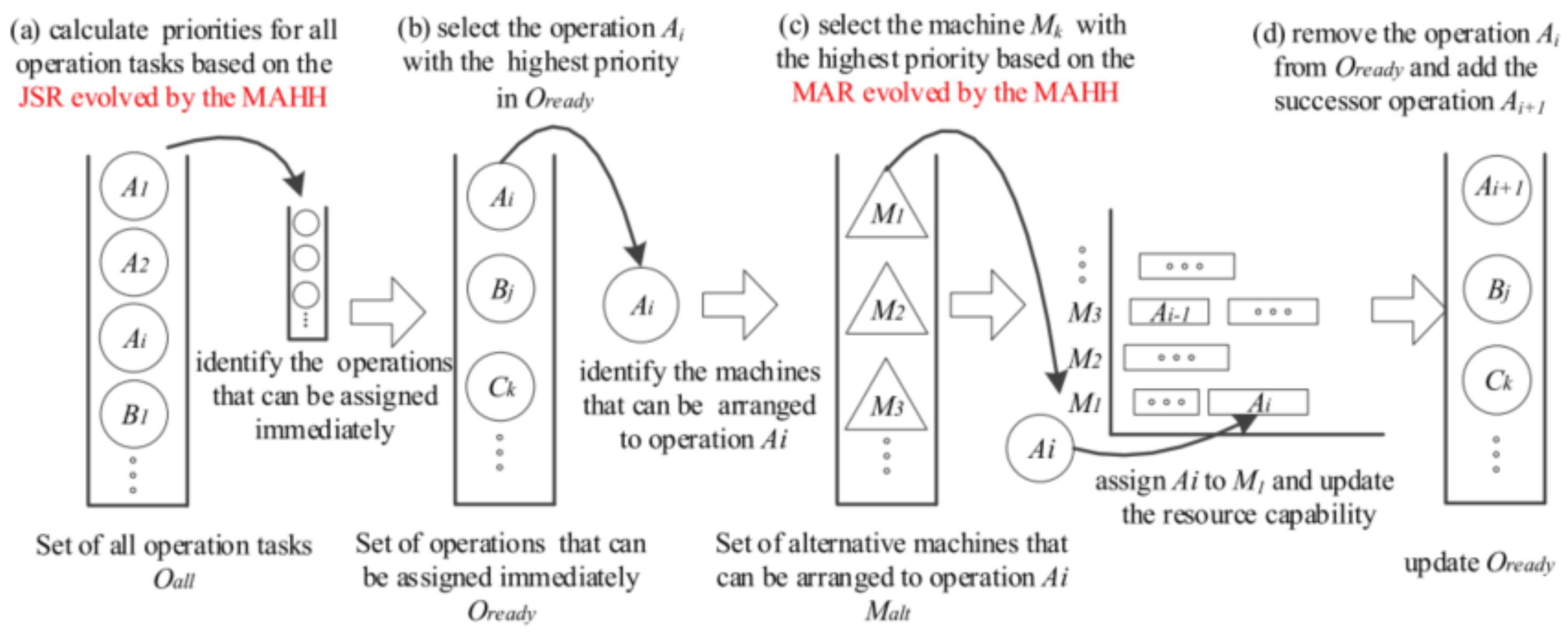
4.3. Application Case of Sequence Learning

As regards the problem illustrated in Figure 7, the product sequence would not change in MA because the FIFO rule was applied to process products sequentially. Meanwhile, the product sequence can change in MB, depending on the machine’s limited capacity and product processing time. If MB exceeds its limited capacity (e.g., K = 3), the remaining products need to enter a buffer station to wait until MB becomes available. If the processing time varies depending on the type of product, unplanned waiting time can become very diverse because of the time gap between the completion time on MA and the arrival time on MB. The product sequence and schedule for MB are different from those for MA. Such a change can lead to a relatively substantial difference between the actual product sequences and schedules and the planned ones, provided that the number of MB increases at the production level. Here, diverse processing time and unplanned waiting time on MB act as uncertainty factors, because they cause complexity in predicting product sequences and schedules. Nevertheless, it is necessary to predict product sequences and their associated time values correctly, even in an environment where the uncertainty factors are incalculable or unforeseeable.
For this purpose, sequence learning can be applied to predict product sequences by learning from historical data. Figure 8 presents a conceptual model for predicting a product sequence using sequence learning, particularly sequence prediction. The inputs of this model are the initial product sequence and arrival rate from the previous machine (the product sequence output from MA in Figure 7), the finishing time of individual products from the previous machine, the processing time of individual products on the designated machine, and the number of products ordered. The outputs of the model are an estimated sequence of products on the MB and its time objective values, including the waiting time and arrival time of individual products on the MB. This model affords information concerning the product positions at certain times and the time when the product arrives in the MB.
Sequence prediction needs to accommodate the changes in sequences accumulatively, because the prediction of the next sequence depends on the previous sequence. Here, the Markov chain (MC) technique was used for sequence prediction; this MC can reflect the causality of the precedent and current status, as well as having shown its superiority in sequence learning. The MC consists of “state”, and “transition” between two states. The state S refers to a product (Pi) in a sequence (Sn), while the transition T represents the probability ( ) between states ( S n to S n + 1 ), which determines whether the product (Pi+1) is located next to Pi. In the MC, the current sequence (Sn) is required to predict the next sequence (Sn+1). Accordingly, (s0, s1, s2, s3, s4, s5, …, sn) is the only function of a state visited in the “Sn” period; this implies that the MC is the set of sequences, as expressed in Equation (1).
P ( S n + 1 = S n + 1 | S n = S n , S n - 1 = S n - 1 , S n - 2 = S n - 2 , )   =   P ( S n + 1 = S n + 1 | S n = S n )
To identify the sequence prediction, a series of transition probability values from the product sequence “n” to “n + 1” is required. This sequence is conditionally independent because the MC can be represented as a matrix of probability vectors (Probss’), as expressed in Equation (2). Based on the given condition, the probability values of the state transition of product (spss’) from the initial state S n to the next state S n + 1 can be derived.
Prob ss = S n S n + 1 sp 11 sp 1 s sp s 1 sp ss
Figure 9 shows an example of the MC for the case illustrated in Figure 7; this chain was implemented using MATLAB. Suppose that the initial sequence is S = (P1, P2, P3, P4, P5, P6, P7, P8, P9, P10); states 1, 2, and 3 are transitioned into themselves with 100% probability, and P1, P2, and P3 are serially entered into MB without change; this is because the maximum capacity of machine 2 is equal to three and, thus, this machine is available for the first three products. Once the number of states exceeds the maximum capacity, the transition probability varies in terms of the processing time on MB and the finishing time on MA. For example, P4 can be transitioned to the seventh position with 80–90% probability, or the sixth position with 10–20% probability; this is because MB was occupied by P1, P2, and P3, and the machine instructed P4 to enter a buffer station for waiting; then, the machine belatedly calls P4 with 80–90% probability after the other three products (e.g., P6, P7, and P8) are already fabricated in the machine. In succession, the remaining states can be transitioned with their probability on the previous states already determined by the MC. In this way, we can determine the entire state, with its transition probability, and predict a product sequence in MB. While a product sequence is predicted, the arrival time of individual products on machines is simultaneously calculated because this time is involved with the product sequence prediction. We than calculate the waiting time and finishing time of each product and, lastly, calculate the total completion time, which corresponds to the total processing time (pfNj) for an order that consists of N products. Equations (3)–(7) express the mathematical equations for the arrival time, waiting time, finishing time, and total completion time, respectively.
Arrival time:
a ij = pf i j 1 + d jj
where pfi(j−1) is the finish time of product (i) in the previous machine (j−1); d jj is the travel time between the previous machine and the designated machine (j); and aij is the arrival time at the designated machine, with 0 ≤ i ≤ N (the number of products ordered).
Waiting time:
w 1 j = 0           , for   i = 1
w ij = i = 1 N 1 p ij a ij ,       for   1   < i     N
with:
w ij = 0   for   w ij 0
w ij   for   w ij > 0
where wij is the waiting time of product-i in machine-j; and pij is the processing time of product-i in machine-j with 0 ≤ i ≤ N.
Finishing time:
pf ij = a ij + w ij + p ij
where pfij is the finish time of product-i in machine-j.
Total completion time:
TC = pfNj
where pfNj is the finish time of product N (the last product) in machine-j (the last machine).
It should be mentioned that even sequence learning is unable to produce a perfect prediction result, owing to the variety of data and the influence of uncertainty. Rather, it forecasts several product sequences with high probability; this is common in data-driven learning approaches; thus, a better prediction of product sequences requires further analysis, as mentioned in Section 4.2. Verification and validation are needed to measure the difference between the predicted and actual results, and to compare the performance of the applied technique with those of other techniques. Sensitivity analysis is useful for determining the change in system conditions by parameter modification and determining a trend from a variety of data.

5. Conclusions

This article reviews the state of the art of prediction and optimization for sequence-driven scheduling in JS-FMSs. For this purpose, this article provides analytical information concerning the current literature in terms of domain, method, objective, sequence type, and uncertainty. This article also discusses the challenges and future directions for research. Future research directions in JS-FMSs include the following: the availability of uncertainty needs to be quantified and modeled explicitly; both holistic and granular algorithms and solutions need to be considered; product sequences need to be incorporated; and sequence learning needs to be applied to realize the prediction-then-optimization stream.
Since the appearance of FMSs in the 1960s, sequencing and scheduling in JS-FMSs have been extensively discussed, and are still being addressed at present. These enormous research efforts prove that JS-FMSs are evolving significantly to improve their responsiveness, flexibility, and productivity, together with increases in their complexity and diversity. As expected, modern FMSs will not stand alone without ICT. ICT contributes to embodying mass customization in modern FMSs, where all products and resources are traced in real time, they are planned and executed autonomously and cooperatively, and their data are exchanged and shared across heterogeneous devices and systems in the control hierarchy. Hence, the convergence of ICT with traditional methodologies in the JS-FMS domain is becoming a critical research stream to improve availability and practicability.
The limitations of this study are as follows: The number of reviewed articles is limited; although more articles have been published in the JS-FMS domain, we only selected articles that were directly involved within the scope of our review, as mentioned in Section 2.2. The other review papers can be useful for understanding FMS technologies from their own perspectives and scopes, as presented in Section 2.1. Our reviews on the product sequence are not analyzed holistically, although we emphasize the significance of the product sequence; this is because the product sequences were only considered in a few articles. In addition, resolutions for overcoming current challenges are partially suggested. We only suggest the possibility of sequence learning, without demonstrating industrial cases that show feasible algorithms and solutions to incorporate the dynamics and uncertainty in JS-FMSs.
In future studies, it will be worthwhile to investigate the feasibility and usability of ICT in FMSs. As the recent smart manufacturing and Industry 4.0 endow resources and products with manufacturing intelligence, this manufacturing intelligence provides data-driven insights and foresights toward dynamic and real-time scheduling prediction and optimization. We plan to investigate and analyze the state of the art of ICT-driven FMSs along with the specification of cutting-edge technologies, including cyber–physical systems, cloud computing and edge computing, industrial Internet of Things, artificial intelligence, and data analytics.

Author Contributions

Conceptualization, P.M. and S.-J.S.; methodology, P.M. and S.-J.S.; resources, P.M.; analysis, P.M.; challenges and future directions, S.-J.S.; writing, P.M. and S.-J.S.; supervision, S.-J.S. All authors have read and agreed to the published version of the manuscript.

Funding

This work was supported by the research fund of Hanyang University (HY-2020).

Acknowledgments

We thank Heejin Seol for technical support via Smart Factory (Variant 4) analysis at the LINC+ Analytical Equipment Center at Hanyang University in Seoul.

Conflicts of Interest

The authors declare no conflict of interest.

References

  1. ElMaraghy, H.; Caggiano, A. Flexible Manufacturing System in the International Academy for Product; Laperrière, L., Reinhart, G., Eds.; CIRP Encyclopedia of Production Engineering; Springer: Berlin/Heidelberg, Germany, 2016. [Google Scholar]
  2. Shivanand, H.K.; Benal, M.M.; Koti, V. Flexible Manufacturing System; New Age International Ltd.: New Delhi, India, 2006. [Google Scholar]
  3. GE Digital team. GE Digital. 2020. Available online: https://www.ge.com/ (accessed on 3 February 2021).
  4. Koh, S.C.L.; Saad, S. Development of a business model for diagnosing uncertainty in ERP environments. Int. J. Prod. Res. 2002, 40, 3015–3039. [Google Scholar] [CrossRef]
  5. Haupt, R. A survey of priority rule based scheduling. Oper. Res. Spektrum 1989, 11, 3–16. [Google Scholar] [CrossRef]
  6. Owen, H.A. Job Shop vs Flow Shop: Can Robots Work for Both? Robotiq. 2017. Available online: https://blog.robotiq.com/ (accessed on 10 February 2021).
  7. Xie, J.; Gao, L.; Peng, K.; Li, X.; Li, H. Review on Flexible Job Shop Scheduling in Effective Methods for Integrated Process Planning and Scheduling; Engineering Applications of Computational Methods; Springer: Berlin/Heidelberg, Germany, 2020; Volume 2. [Google Scholar]
  8. Baker, K.R.; Trietsch, D. Principles of Scheduling and Sequencing; John Wiley & Sons, Inc.: Hoboken, NJ, USA, 2009. [Google Scholar]
  9. Hall, N.G.; Magazine, M. Scheduling and sequencing. In Encyclopedia of Operations Research and Management Science; Gass, S.I., Michael, C.F., Eds.; Springer: Boston, MA, USA, 2013. [Google Scholar]
  10. Swamidass, P.M. (Ed.) Job Sequence Rules. Encyclopedia of Production and Manufacturing Management; Kluwer Academic Publishers: Boston, MA, USA, 2000. [Google Scholar]
  11. Zhu, X.; Wilhelm, W.E. Scheduling and lot sizing with sequence dependent setup: A literature review. IIE Trans. 2006, 38, 987–1007. [Google Scholar] [CrossRef]
  12. Chaudhry, I.A.; Khan, A.A. A research survey: Review of flexible job shop scheduling techniques. Int. Trans. Oper. Res. 2016, 23, 551–591. [Google Scholar] [CrossRef]
  13. Gao, K.; Cao, Z.; Zhang, L.; Chen, Z.; Han, Y.; Pan, Q. A review on swarm intelligence and evolutionary algorithms for solving flexible job shop scheduling problems. IEEE/CAA J. Autom. Sin. 2019, 6, 904–916. [Google Scholar] [CrossRef]
  14. Demir, Y.; İşleyen, S.K. Evaluation of mathematical models for flexible job-shop scheduling problems. Appl. Math. Model. 2013, 37, 977–988. [Google Scholar] [CrossRef]
  15. Zhang, J.; Ding, G.; Zou, Y.; Qin, S.; Fu, J. Review of job shop scheduling research and its new perspectives under Industry 4.0. J. Intell. Manuf. 2019, 30, 1809–1830. [Google Scholar] [CrossRef]
  16. Rasheed, F.; Wahid, A. Sequence generation for learning: A transformation from past to future. Int. J. Inf. Learn. Technol. 2019, 36, 434–452. [Google Scholar] [CrossRef]
  17. Akbar, M.; Irohara, T. Scheduling for sustainable manufacturing: A review. J. Clean. Prod. 2018, 205, 866–883. [Google Scholar] [CrossRef]
  18. Shin, S.J.; Kim, Y.M.; Meilanitasari, P. A holonic-based self-learning mechanism for energy-predictive planning in machining processes. Processes 7 2019, 10, 739. [Google Scholar] [CrossRef] [Green Version]
  19. Shen, L.; Pérès, S.D.; Neufeldd, J.N. Solving the flexible job shop scheduling problem with sequence-dependent setup times. Eur. J. Oper. Res. 2018, 265, 503–516. [Google Scholar] [CrossRef]
  20. Luo, D.L.; Wu, S.X.; Li, M.Q.; Yang, Z. Ant colony optimization with local search applied to the Flexible Job Shop Scheduling Problems. Int. Conf. Commun. Circuits Syst. 2008, 1015–1020. [Google Scholar]
  21. Pezzella, F.; Morganti, G.; Chiaschetti, G. A genetic algorithm for the flexible job-shop scheduling problem. Comput. Oper. Res. 2008, 35, 3202–3212. [Google Scholar] [CrossRef]
  22. Vinod, V.; Sridharan, R. Scheduling a dynamic job shop production system with sequence-dependent setups: An experimental study. Robot. Comput. Integr. Manuf. 2008, 24, 435–449. [Google Scholar] [CrossRef]
  23. Qiu, H.; Zhou, W.; Wang, H. A genetic algorithm-based approach to flexible job-shop scheduling problem. In Proceedings of the 2009 Fifth International Conference on Natural Computation, Tianjin, China, 14–16 August 2009. [Google Scholar]
  24. Song, L.; Xu, X. Flexible job shop scheduling problem solving based on genetic algorithm with chaotic local search. In Proceedings of the 2010 Sixth International Conference on Natural Computation, Yantai, China, 10–12 August 2010. [Google Scholar]
  25. Wang, S.; Yu, J. An effective heuristic for flexible job-shop scheduling problem with maintenance activities. Comput. Ind. Eng. 2010, 59, 436–447. [Google Scholar] [CrossRef]
  26. Bagheri, A.; Zandieh, M. Bi-criteria flexible job-shop scheduling with sequence-dependent setup times variable neighborhood search approach. J. Manuf. Syst. 2011, 30, 8–15. [Google Scholar] [CrossRef]
  27. Moslehi, G.; Mahnam, M. A pareto approach to multi-objective flexible job-shop scheduling problem using particle swarm optimization and local search. Int. J. Prod. Econ. 2011, 129, 14–22. [Google Scholar] [CrossRef]
  28. Wan, M.; Xu, X.; Nan, J. Flexible job-shop scheduling with integrated genetic algorithm. In Proceedings of the Fourth International Workshop on Advanced Computational Intelligence, Wuhan, China, 19–21 October 2011. [Google Scholar]
  29. Xue, G.; Offodile, O.F.; Zhou, H.; Troutt, M.D. Integrated production planning with sequence-dependent family setup times. Int. J. Prod. Econ. 2011, 131, 674–681. [Google Scholar] [CrossRef]
  30. Agrawal, R.; Pattanaik, L. Scheduling of a flexible job shop using a multi objective genetic algorithm. J. Adv. Manag. Res. 2012, 9, 178–188. [Google Scholar] [CrossRef]
  31. Gao, K.; Suganthan, P.; Chua, T. Pareto-based discrete harmony search algorithm for flexible job shop scheduling. In Proceedings of the 2012 12th International Conference on Intelligent Systems Design and Applications (ISDA), Kochi, India, 27–29 November 2012. [Google Scholar]
  32. Özgüven, C.; Yavuz, Y.; Özbakır, L. Mixed integer goal programming models for the flexible job-shop scheduling problems with separable and non-separable sequence dependent setup times. Appl. Math. Model. 2012, 36, 846–858. [Google Scholar] [CrossRef]
  33. Xiong, J.; Xing, L.N.; Chen, Y.W. Robust scheduling for multi-objective flexible job-shop problems with random machine breakdowns. Int. J. Prod. Econ. 2013, 141, 112–126. [Google Scholar] [CrossRef]
  34. Xu, Z.; Li, Y.; Zhang, J.; Cheng, H.; Jiang, S.; Tang, W. A dynamic assembly model for assembly sequence planning of complex product based on polychromatic sets theory. Assem. Autom. 2012, 32, 152–162. [Google Scholar] [CrossRef]
  35. Chen, B.; Matis, T.I. A flexible dispatching rule for minimizing tardiness in job shop scheduling. Int. J. Prod. Econ. 2013, 141, 360–365. [Google Scholar] [CrossRef]
  36. Kechadi, M.T.; Low, K.S.; Goncalves, G. Recurrent neural network approach for cyclic job shop scheduling problem. J. Manuf. Syst. 2013, 32, 689–699. [Google Scholar] [CrossRef] [Green Version]
  37. Yuan, Y.; Xu, H.; Yang, J. A hybrid harmony search algorithm for the flexible job shop scheduling problem. Appl. Soft Comput. 2013, 13, 3259–3272. [Google Scholar] [CrossRef]
  38. Liu, T.; Chen, Y.; Chou, J. Solving distributed and flexible job-shop scheduling problems for a real-world fastener manufacturer. IEEE Access 2014, 2, 1598–1606. [Google Scholar]
  39. Song, X.; Zhou, W.; Pan, X.; Feng, K. Disassembly sequence planning for electro-mechanical products under a partial destructive mode. Assem. Autom. 2014, 34, 106–114. [Google Scholar] [CrossRef]
  40. Moghadam, A.; Wong, K.; Piroozfard, H. An efficient genetic algorithm for flexible job-shop scheduling problem. In Proceedings of the 2014 IEEE International Conference on Industrial Engineering and Engineering Management, Bandar Sunway, Malaysia, 9–12 December 2014. [Google Scholar]
  41. Rossi, A. Flexible job shop scheduling with sequence-dependent setup and transportation times by ant colony with reinforced pheromone relationships. Int. J. Prod. Econ. 2014, 153, 253–267. [Google Scholar] [CrossRef]
  42. Abdelmaguid, T.F. A neighborhood search function for flexible job shop scheduling with separable sequence-dependent setup times. Appl. Math. Comput. 2015, 260, 188–203. [Google Scholar] [CrossRef]
  43. Palacios, J.J.; González, M.A.; Vela, C.R.; Rodríguez, I.G.; Puente, J. Genetic tabu search for the fuzzy flexible job shop problem. Comput. Oper. Res. 2015, 54, 74–89. [Google Scholar] [CrossRef] [Green Version]
  44. Ham, A.M.; Cakici, E. Flexible job shop scheduling problem with parallel batch processing machines: MIP and CP approaches. Comput. Ind. Eng. 2016, 102, 160–165. [Google Scholar] [CrossRef]
  45. Torkaman, S.; Ghomi, S.M.T.F.; Karimi, B. Multi-stage multi-product multi-period production planning with sequence-dependent setups in closed-loop supply chain. Comput. Ind. Eng. 2017, 113, 602–613. [Google Scholar] [CrossRef]
  46. Gong, G.; Deng, Q.; Gong, X.; Liu, W.; Ren, Q. A new double flexible job-shop scheduling problem integrating processing time, green production, and human factor indicators. J. Clean. Prod. 2018, 174, 560–576. [Google Scholar] [CrossRef]
  47. Jamrus, T.; Chien, C.; Gen, M.; Sethanan, K. Hybrid particle swarm optimization combined with genetic operators for flexible job-shop scheduling under uncertain processing time for semiconductor manufacturing. IEEE Trans. Semicond. Manuf. 2018, 31, 32–41. [Google Scholar] [CrossRef]
  48. Zhang, S.; Wang, S. Flexible assembly job-shop scheduling with sequence-dependent setup times and part sharing in a dynamic environment: Constraint programming model, mixed-integer programming model, and dispatching rules. IEEE Trans. Eng. Manag. 2018, 65, 487–504. [Google Scholar] [CrossRef]
  49. Novas, J.M. Production scheduling and lot streaming at flexible job-shops environments using constraint programming. Comput. Ind. Eng. 2019, 136, 252–264. [Google Scholar] [CrossRef]
  50. Li, Z.C.; Qian, B.; Hu, R.; Chang, L.L.; Yang, J.B. An elitist nondominated sorting hybrid algorithm for multi-objective flexible job-shop scheduling problem with sequence-dependent setups. Knowl. Based Syst. 2019, 173, 83–112. [Google Scholar] [CrossRef]
  51. Huang, X.; Yang, L. A hybrid genetic algorithm for multi-objective flexible job shop scheduling problem considering transportation time. Int. J. Intell. Comput. Cybern. 2019, 12, 154–174. [Google Scholar] [CrossRef]
  52. Wu, C.C.; Azzouz, A.; Chung, I.H.; Lin, W.C.; Said, L.B. A two-stage three-machine assembly scheduling problem with deterioration effect. Int. J. Prod. Res. 2019, 57, 6634–6647. [Google Scholar] [CrossRef]
  53. Zhang, Y.; Zhu, H.; Tang, D. An improved hybrid particle swarm optimization for multi-objective flexible job-shop scheduling problem. Kybernetes 2019, 49, 2873–2892. [Google Scholar] [CrossRef]
  54. Zhao, M.; Guo, X.; Zhang, X.; Fang, Y.; Ou, Y. ASPW-DRL: Assembly sequence planning for work pieces via a deep reinforcement learning approach. Assem. Autom. 2019, 40, 65–75. [Google Scholar] [CrossRef]
  55. Zhou, Y.; Yang, J.J.; Zheng, L.Y. Multi-agent based hyper-heuristics for multi objective flexible job shop scheduling: A case study in an aero-engine blade manufacturing plant. IEEE Access 2019, 7, 21147–21176. [Google Scholar] [CrossRef]
  56. Abreu, L.; Prata, B. A genetic algorithm with neighborhood search procedures for unrelated parallel machine scheduling problem with sequence-dependent setup times. J. Model. Manag. 2020, 15, 809–828. [Google Scholar] [CrossRef]
  57. Defersha, F.M.; Rooyani, D. An efficient two-stage genetic algorithm for a flexible job-shop scheduling problem with sequence dependent attached/detached setup, machine release date and lag-time. Comput. Ind. Eng. 2020, 147, 106605. [Google Scholar] [CrossRef]
  58. Fattahi, P.; Bagheri Rad, N.; Daneshamooz, F.; Ahmadi, S. A new hybrid particle swarm optimization and parallel variable neighborhood search algorithm for flexible job shop scheduling with assembly process. Assem. Autom. 2020, 40, 419–432. [Google Scholar] [CrossRef]
  59. Gu, X.; Huang, M.; Liang, X. A discrete particle swarm optimization algorithm with adaptive inertia weight for solving multi objective flexible job-shop scheduling problem. IEEE Access 2020, 8, 33125–33136. [Google Scholar] [CrossRef]
  60. Lin, C.S.; Li, P.Y.; Wei, J.M.; Wu, M.C. Integration of process planning and scheduling for distributed flexible job shops. Comput. Oper. Res. 2020, 124, 105053. [Google Scholar] [CrossRef]
  61. Luo, S. Dynamic scheduling for flexible job shop with new job insertions by deep reinforcement learning. Appl. Soft Comput. J. 2020, 91, 106208. [Google Scholar] [CrossRef]
  62. Wang, Y.; Xie, N. Flexible flow shop scheduling with interval grey processing time. Grey Syst. Theory Appl. 2020, 2043–9377. [Google Scholar]
  63. Wu, C.C.; Gupta, J.N.D.; Cheng, S.R.; Lin, B.M.T.; Yip, S.H.; Lin, W.C. Robust scheduling for a two-stage assembly shop with scenario-dependent processing times. Int. J. Prod. Res. 2020, 2020, 1–16. [Google Scholar] [CrossRef]
  64. Wu, C.C.; Bai, D.; Zhang, X.; Cheng, S.R.; Lin, J.C.; Wu, Z.L.; Lin, W.C. A robust customer order scheduling problem along with scenario-dependent component processing times and due dates. J. Manuf. Syst. 2021, 58, 291–305. [Google Scholar] [CrossRef]
  65. Wu, C.C.; Zhang, X.; Azzouz, A.; Shen, W.L.; Cheng, S.R.; Hsu, P.H.; Lin, W.C. Metaheuristics for two-stage flow-shop assembly problem with a truncation learning function. Eng. Optim. 2021, 53, 843–866. [Google Scholar] [CrossRef]
  66. Nouri, H.E.; Driss, O.B.; Ghédira, K. Solving the flexible job shop problem by hybrid metaheuristics-based multi agent model. J. Ind. Eng. Int. 2018, 14, 1–14. [Google Scholar] [CrossRef]
  67. Candan, G.; Yazgan, H.R. Genetic algorithm parameter optimization using Taguchi method for a flexible manufacturing system scheduling problem. Int. J. Prod. Res. 2015, 53, 897–915. [Google Scholar] [CrossRef]
  68. Udhayakumar, P.; Kumanan, S. Sequencing and scheduling of job and tool in a flexible manufacturing system using ant colony optimization algorithm. Int. J. Adv. Manuf. Technol. 2010, 50, 1075–1984. [Google Scholar] [CrossRef]
  69. Kantor, I.; Robineau, J.L.; Bütün, H.; Maréchal, F. A mixed integer linear programming formulation for optimizing multi scale material and energy integration. Front. Energy Res. 2020, 8, 49. [Google Scholar] [CrossRef]
  70. NCSS, NCSS Statistical Software: Chapter 482: Mixed Integer Linear Programming. 2021. Available online: https://www.ncss.com/software/ncss/ncss-documentation/ (accessed on 3 March 2021).
  71. Hurwitz, J.; Kirsch, D. Machine Learning IBM Limited Edition; John Wiley & Sons, Inc.: Hoboken, NJ, USA, 2018. [Google Scholar]
  72. Greeff, G.; Ghoshal, R. (Eds.) Production scheduling, management and control. In Practical E-Manufacturing and Supply Chain Management; Elsevier: Amsterdam, The Netherlands, 2004; pp. 243–269. [Google Scholar]
  73. Pena, P.N.; Costa, T.A.; Silva, R.S.; Takahashi, R.H. Control of flexible manufacturing systems under model uncertainty using supervisory control theory and evolutionary computation schedule synthesis. Inf. Sci. 2016, 329, 491–502. [Google Scholar] [CrossRef]
  74. Akpan, E. Job shop sequencing problems via network scheduling technique. Int. J. Oper. Prod. Manag. 1996, 16, 76–86. [Google Scholar] [CrossRef]
  75. Chapter II: Sequencing and scheduling–An Overview. 2020. Available online: http://courseware.cutm.ac.in/wp-content/uploads/2020/06/sequencing-pdf.pdf (accessed on 10 February 2021).
  76. Elmachtoub, A.N.; Grigas, P. Smart “Predict, then Optimize”. arXiv 2020, arXiv:1710.08005. [Google Scholar]
  77. Wazed, M.A.; Ahmed, S.; Yusoff, N. Uncertainty factors in real manufacturing environment. Aust. J. Basic Appl. Sci. 2009, 3, 342–351. [Google Scholar]
  78. Roy, C.J.; Oberkampf, W.L. A comprehensive framework for verification, validation, and uncertainty quantification in scientific computing. Comput. Methods Appl. Mech. Eng. 2011, 200, 2131–2144. [Google Scholar] [CrossRef]
  79. Mahadevan, S.; Liang, B. Error and uncertainty quantification and sensitivity analysis in mechanics computational models. Int. J. Uncertain. Quantif. 2011, 1, 147–161. [Google Scholar] [CrossRef]
  80. Nannapaneni, S.; Mahadevan, S.; Rachuri, S. Performance evaluation of a manufacturing process under uncertainty using Bayesian networks. J. Clean. Prod. 2016, 113, 947–959. [Google Scholar] [CrossRef] [Green Version]
  81. Monostori, L. AI and machine learning techniques for managing complexity, changes and uncertainties in manufacturing. Eng. Appl. Artif. Intell. 2003, 16, 277–291. [Google Scholar] [CrossRef]
  82. Brussel, V.H.; Wyns, J.; Valckenaers, P.; Bongaerts, L.; Peeters, P. Reference architecture for holonic manufacturing systems: PROSA. Comput. Ind. 1998, 37, 255–274. [Google Scholar] [CrossRef]
  83. Shen, W.; Hao, Q.; Yoon, H.J.; Norrie, D.H. Applications of agent-based systems in intelligent manufacturing: An updated review. Adv. Eng. Inform. 2019, 20, 415–431. [Google Scholar] [CrossRef]
  84. Norrie, D.H.; Walker, S.S.; Brennan, R.W. Holonic job shop scheduling using a multiagent system. IEEE Intell. Syst. 2005, 20, 50–57. [Google Scholar]
  85. Priore, P.; Fuente, D.D.L.; Puente, J.; Parreno, J. A comparison of machine-learning algorithms for dynamic scheduling of flexible manufacturing systems. Eng. Appl. Artif. Intell. 2006, 19, 247–255. [Google Scholar] [CrossRef]
  86. Sun, R. Introduction to Sequence Learning, in Sequence Learning Paradigms, Algorithms, and Applications; Springer: Berlin/Heidelberg, Germany, 2001; pp. 1–12. [Google Scholar]
Figure 1. Sequence type in production in an FMS.
Processes 09 01391 g001
Figure 2. Research methodology.
Processes 09 01391 g002
Figure 3. Research framework.
Processes 09 01391 g003
Figure 4. Random dispatching rule based on priority: (a) calculate priorities, (b) select the operation, (c) select the machine, (d) remove the operation [55].
Processes 09 01391 g004
Figure 5. Sequence type in production in an FMS [49].
Processes 09 01391 g005
Figure 6. Framework for sequence-driven scheduling in a JS-FMS.
Processes 09 01391 g006
Figure 7. Example of a JS-FMS with uncertainty.
Processes 09 01391 g007
Figure 8. Concept of sequence-learning-based product sequence prediction.
Processes 09 01391 g008
Figure 9. Example of product sequence prediction using a Markov chain.
Processes 09 01391 g009
Table 2. List of article sources.
Name of Journal or Proceeding Number of Articles
2008 International Conference on Communications, Circuits, and Systems1
2009 Fifth International Conference on Natural Computation1
2010 Sixth International Conference on Natural Computation1
2012 12th International Conference on Intelligent Systems Design and Applications (ISDA)1
2014 IEEE International Conference on Industrial Engineering and Engineering Management1
Applied Mathematical Modelling1
Applied Mathematics and Computation1
Assembly Automation4
Computers & Industrial Engineering5
Computers & Operations Research3
Engineering Optimization1
European Journal of Operational Research1
Applied Soft Computing1
Grey Systems: Theory and Application1
IEEE Access3
IEEE Transactions on Automation Science and Engineering1
IEEE Transactions on Engineering Management1
IEEE Transactions on Semiconductor Manufacturing1
Industrial Robot1
International Journal of Intelligent Computing and Cybernetics1
International Journal of Production Economics5
International Journal of Production Research2
Journal of Advances in Management Research1
Journal of Cleaner Production1
Journal of Manufacturing Systems3
Journal of Modelling in Management1
Knowledge-Based Systems1
Kybernetes1
Robotics and Computer-Integrated Manufacturing1
Publisher’s Note: MDPI stays neutral with regard to jurisdictional claims in published maps and institutional affiliations.

