Quality-Analysis-Based Process Monitoring for Multi-Phase Multi-Mode Batch Processes

Abstract

In batch processing, not only the characteristics of different phases are different, but also there may be different characteristics between batches. These characteristics of different phases and batches will have different effects on the final product quality. In order to enhance the safety of batch processes, it is necessary to establish an appropriate monitoring system to monitor the production process based on quality-related information. In this work, based on multi-phase and multi-mode quality prediction, a new quality-analysis-based process-monitoring strategy is developed for batch processes. Firstly, the time-slice models are established to determine the critical-to-quality phases. Secondly, a multi-phase residual recursive model is established using each quality residual of the phase mean models. Subsequently, a new process-monitoring strategy based on quality analysis is proposed for a single mode. After that, multi-mode quality analysis is carried out to judge the relevance between the historical modes and the new mode. Further, online quality prediction is achieved applying the selected model based on multi-mode quality analysis, and an according process-monitoring strategy is developed. The simulation results show the availability of this method for multi-phase multi-mode batch processes.

1. Introduction

Batch process products play an increasingly important role in modern human life. In order to meet the ever-changing market demand of modern society, the safe and reliable operation of batch processes and continuous and stable product quality have gradually become the focus of attention in the processing industry [1,2]. The characteristics of batch operation processes are more complex than that of continuous industrial processes and have more abundant statistical characteristics. In order to enhance the safety of the batch production process and its control system, it is urgent to establish a suitable process-monitoring system to monitor the production process.

Currently, data-driven methods [3,4,5] of extracting information from process data and modeling monitoring have become a hotspot in process-monitoring research. With the advancement of sensor technology, almost all industrial objects are equipped with different types of sensing devices. This results in a large amount of data being obtained in an industrial process. The data-driven methods extract information hidden in data by analyzing and mining collected industrial data, which may help reveal the operation mode of the industrial process and trace the fault reasons. In recent years, data-driven methods are continuously developed and perfected, batch process monitoring and fault diagnosis technologies based on data-driven methods have increasingly become research hotspots of people, and theories of the batch process monitoring and fault diagnosis technologies are continuously and deeply developed.

Multivariate statistical analysis methods do not require the acquisition of process mechanism knowledge; they only require the use of historical data to build models. These methods can effectively extract key information in data, eliminate redundancy and remarkably reduce data dimensionality so that the process running state can be directly displayed in a two-dimensional statistical monitoring graph. Before the 1990s, researchers have generally simply treated batch processes as special continuous processes of limited duration, with no theoretical system of research specifically directed to batch process monitoring. Due to the essential difference of the characteristics of the batch process and the continuous process, a satisfactory effect is difficult to obtain in the batch process.

Aiming at the three-dimensional data characteristics of the batch process, a trilinear decomposition model can be established to directly investigate the three-dimensional data structure [6]. The data are stored and analyzed by using a trilinear decomposition model, and structural information of the data can be retained. In summary, there are six different two-dimensional matrix unfolding modes [7], which mainly reflect the different arrangement modes inside the data.

Nomikos [8,9,10] proposed multi-way principal components analysis (MPCA) and multi-way partial least squares (MPLS) methods, innovatively extending the successful application of multivariate statistical analysis methods to batch processes. Different internationally academic institutions and teams, including Wold professor [11] of Umea University, English Martin professor [12] of Newcastle University, proposed their own methodology, which facilitates the study of batch process monitoring. Corresponding models for monitoring have been established based on the model under normal conditions. When influenced by abnormal disturbances, the process variable correlations are changed, thereby deviating from the laws and characteristics under normal conditions. Corresponding multivariate statistics are calculated and compared with the monitoring control limits defined in advance, and the occurrence of abnormal working conditions can be detected.

In the batch process, the multi-phase nature is another important nature. In recent years, many scholars have conducted considerable research into process monitoring and quality analysis of batch processes [13,14,15]. Most researches were carried out by establishing different models to obtain different characteristics and dividing a cycle of a batch into phases, due to the cognition that the correlation of variables in the same phase is similar, and the correlation of variables in different phases is very different. Some scholars study the characteristics of the phases, e.g., the problem of transitions between adjacent phases [16] and the problem of non-uniform durations [17]. In addition, the scholars suggested that phases contribute to the final quality together, and individual phase models should be connected in some way during the modeling process. Therefore, a recursive quality regression method aiming at the multi-phase characteristics of the batch process was proposed [18], where the regression on the process variables in the current phase and the residual quality obtained in the previous phase was carried out to extract important quality information between the phase.

In addition, due to the influence of various factors, there are multi-mode characteristics in the batch process. In the whole operation process, process changes in batch direction lead to different process states and different process characteristics. In this way, monitoring and quality prediction for only one process state may lead to inaccurate analysis and monitoring results. In order to solve this problem, some scholars proposed to build an integrated model that can include both the common model and the specific model [19]. However, these methods barely evaluate the changes along the batch direction, in which models are in general updated arbitrarily, decreasing the efficiency of the monitoring system, as well as increasing the chance of introducing disturbances into the process model. Some scholars have proposed a specific modeling method for a specific process state [20]. However, the process variation along the batch direction may be too slow to be divided into several states. In addition, in the batch production process, when a new mode is generated, the corresponding model is built in the mode library and saved in the mode library. However, the relationship between these modes is not analyzed and judged. As new modes are generated one after another, all new modes must be saved, which makes the mode library larger and larger. Therefore, a quality prediction method based on the relationship between modes is proposed to extract information from historical modes [21].

In recent years, monitoring of multiple characteristics of batch processes has also been the direction of many scholars. A process-monitoring method based on multi-mode Fisher discriminant analysis to solve the problem of multi-mode monitoring of batch process was proposed [22], which overcomes the limitation of the single operation mode assumption. Taking the whole batch trajectory as the research object, based on the dynamic time warping method, the obtained data are automatically classified from the perspective of data distribution to reflect the differences in batch direction. For the batch process with multi-phase characteristics, a two-phase PLS regression model based on phase analysis and different statistical analyses was proposed [23]. At the first level, multiple PLS models are used to monitor a single point in time. At the second level, the final quality is predicted. Through these two different levels of models, real-time monitoring and accurate quality prediction are organically combined. Due to the calibration and modeling problems caused by operation switching (or moving to different phases), a new evolutionary PLS method is proposed, which can be used to predict intermediate quality measurement and to detect process faults avoiding false positives [24].

In this work, both multi-phase quality analysis and multi-mode quality analysis are conducted at the same time to develop a comprehensive process-monitoring strategy based on the quality prediction of batch processes. The multi-phase and multi-mode batch process concerned here involves variety in two directions. One is the multi-phase direction, the other is the multi-mode direction, and the processing methods of the two directions are different due to different process characteristics. In the multi-phase direction, the phase residual recursive model is unitized to connect the contributions of the successive phases on the final quality together, while in the multi-mode direction, the relationship between the current mode and the historical mode is analyzed and extracted to obtain more quality-related information for quality prediction. Firstly, the time-slice modeling method and the goodness-of-fit index are used to analyze the influence of different phases on the final quality and identify the critical-to-quality phases. Then, the phase mean model is introduced to analyze the phase characteristics and monitor the phase based on quality information. After that, single modes are analyzed, where the residual regression model of each phase is established with the quality variables of the current phase and the quality residual of the previous phase, and the current mode is predicted and monitored. In addition, for the quality prediction and monitoring of multiple modes, it is emphasized to extract the relationship between historical mode and new mode by between-mode modeling. This model contains more modal quality-related information and can better predict and monitor multiple modes. Finally, the strategy is applied to an injection molding process to illustrate the effectiveness of the strategy.

The rest of this paper includes four parts: the proposed method is presented in Section 2, including critical-to-quality phase identification, phase mean model, multi-phase residual recursive modeling for a single mode, between-mode modeling for multiple modes and model comparison and selection. In Section 3, the injection molding process is briefly introduced, and the method used is illustrated through an example to obtain the results and make a comparative analysis. At last, the conclusion is drawn.

2. Methodology

2.1. Critical-to-Quality Phase Identification Based on Time-Slice Model

In the batch process, there will be different process requirements in the whole operation process, causing obvious phase characteristics. The batch process can be divided into several phases according to process variable relevance. Due to the phase characteristic, there is no significant change in the correlation between process variables and quality variables at different sampling times in the same phase; that is to say, the effect of process operation behavior on quality is similar in the same phase. However, in different phases, the influences of process variables on quality are different, and they show different statistical relationships. Because of the above characteristics of batch processes, a phase that has a significant contribution to the final quality is defined as the critical-to-quality phase. There may be several critical-to-quality phases in the batch process. If production has multiple quality variables, the critical-to-quality phases may be different or the same for different quality variables, depending on the characteristics of the process. Therefore, it is important to find out the critical-to-quality phases that contribute the most to the quality change.

Batch process data are generally represented by $X(I\times J_x\times K)$, where $I$ is the number of batches, $J_x$ is the number of process variables, and $K$ is the sample times. The quality data is generally represented by $Y(I\times J_y)$, where $J_y$ is the number of measurement values. The measurement values of all $J_x$ variables at the sampling interval k (k = 1,…,K) are stored in $X_k(I\times J_x)$, which is called the kth time slice of $X_k$. The relationship between process variables and quality variables at time interval k can be collected from matrices $X_k$ and $Y$. By applying PLS, the kth time-slice PLS model is realized.

$$\begin{array}{l}{X}_k=T_k{P}_k^{\mathrm{T}}+E_k\\ Y=U_k{Q}_k^{\mathrm{T}}+F_k\end{array}$$

(1)

The previous model can be expressed by the regression model as:

$${\widehat{Y}}_k=X_k{B}_k$$

(2)

Where $T_k$ and $U_k$ are the score matrices, ${\mathbf{P}}_k$ and $Q_k$ are the loading matrices, $E_k$ and $F_k$ are the residual matrices, $B_k$ is the regression parameter matrix, k = 1,2,…,K, and ${\widehat{Y}}_k$ is the predicted quality. When considering a single quality variable $y\left(I\times 1\right)$, the regression model can be simply expressed as:

$${\widehat{y}}_k=X_k{\mathsf{\beta }}_k$$

(3)

${\mathsf{\beta }}_k$ is the regression parameter and ${\widehat{y}}_k$ is the predicted quality at the current time. In the regression model, the number of latent variables needs to be determined, and the four-fold cross-validation method is used in this work [25,26].

In this paper, the index R², which is used to describe the goodness of fit of the regression model in the field of multivariable linear regression, is used to measure the influence of each time slice on the final quality. Those time slices with high R² are identified to be critical to quality, and the phases with these time slices are identified as critical-to-quality phases. The kth sampling time is defined. The prediction accuracy $R_k^2$ of the quality prediction model for the quality index y is as follows:

$$R_k^2=\frac{{\displaystyle \sum _{i=1}^I{({\widehat{y}}_{i,k}-\overline{y})}^2}}{{\displaystyle \sum _{i=1}^I{(y_i-\overline{y})}^2}}$$

(4)

where $y_i$ is the quality variable measurement value of the ith batch operation in the test batch, ${\widehat{y}}_{i,k}$ is the model prediction value of the ith batch operation quality variable of the predicted kth time slice, and $\overline{y}$ is the average value of the quality variable measurement value of the test batch. The value range of $R_k^2$ is 0–1. When $R_k^2$ approaches 1, it indicates that the accuracy of the quality prediction model is high, which indicates that the bigger impact on the quality variables is in this phase. On the contrary, the smaller the $R_k^2$ is, the smaller the impact on quality variables is. Therefore, by observing the $R_k^2$ size of different phases, the critical-to-quality phases in the batch process can be determined.

2.2. Phase Mean Model

According to the characteristics of batch processes, the whole process can be divided into several phases. There are obvious differences in the process variables in different phases, and the same phase can be almost considered to have similar process variables. In this work, for the multi-phase and multi-mode quality analysis, it is supposed that the characteristics along the time direction in each phase are constant. It is considered to establish such a model that can represent the process variable relationships of the entire phase. The phase mean model is achieved as follows.

First, the average variable matrix is calculated in phase c,

$${\overline{X}}_c={\displaystyle \sum _{k=1}^{K_c}{X}_{k,c}}/K_c$$

(5)

where $K_c$ is the data length of phase c. $X_{k,c}$ is the data matrix of the process variables at the k moment in phase c. Thus, ${\overline{X}}_c$ is the average variable matrix of phase c.

Within phase c, phase regression models can be built using the PLS method,

$$\begin{array}{l}{\overline{X}}_c=T_c{P}_c^{\mathrm{T}}+E_c\\ Y=U_c{Q}_c^{\mathrm{T}}+F_c\end{array}$$

(6)

The previous model can be expressed by the regression form as:

$${\widehat{Y}}_c={\overline{X}}_c{B}_c$$

(7)

where the concepts of $T_c$, $U_c$, $P_c$, $E_c$, $F_c$, and $B_c$ are the same as those of the time-slice model, except that each matrix is with the meaning of the phase mean. ${\widehat{Y}}_c$ is the predicted quality of the cth phase mean model. When a single quality variable $y\left(I\times 1\right)$ is considered, the regression model can be simply expressed as:

$${\widehat{y}}_c={\overline{X}}_c{\mathsf{\beta }}_c$$

(8)

where ${\mathsf{\beta }}_c$ is the regression parameter, and at present $T_c$ is a matrix of the dimension $I\times H$, $U_c$ is a matrix of the dimension $I\times 1$.

For process monitoring, Hotelling-T² and SPE statistics are calculated in systematic and residual subspaces, respectively [8,27].

$${\mathit{T}}_c{}^2=x_c{}^{\mathrm{T}}{R}_c{(\frac{T_c{}^{\mathrm{T}}{T}_c}{I-1})}^{-1}{\mathrm{R}}_c{}^{\mathrm{T}}{x}_c$$

(9)

$$\mathit{S}\mathit{P}{\mathit{E}}_c={\Vert {\tilde{x}}_c\Vert }^2={\Vert (I_{J_x}-P_c{R}_c{}^{\mathrm{T}})x_c\Vert }^2$$

(10)

where ${\tilde{x}}_c$ is the residual vector; $R_c=W_c{(P_c{}^{\mathrm{T}}{W}_c)}^{-1}$; $W_c$ is the weight matrix; ${\mathit{\delta }}_{{\mathit{T}}_c{}^2}(\alpha )$ is the control limit with $\alpha$ confidence of ${\mathit{T}}_c{}^2$; and $\mathit{S}\mathit{P}{\mathit{E}}_c(\alpha )$ is the $\alpha$ confidence limit of SPE. The detailed properties and calculations can be found in reference [28].

The corresponding control limits are:

$${\mathit{\delta }}_{{\mathit{T}}_c{}^2}(\alpha )=\frac{H(I^2-1)}{I(I-H)}{\mathit{F}}_{c\alpha }(H,I-H)$$

(11)

$$\mathit{S}\mathit{P}{\mathit{E}}_c(\alpha )={\mathit{g}}_c{\mathit{\chi }}_{h,\alpha }^2$$

(12)

where ${\mathit{F}}_{c\alpha }(H,I-H)$ is the $\mathit{F}$ distribution with $\alpha$ confidence and $H$ and $I-H$ degrees of freedom, and $H$ is the number of retained latent variables; ${\mathit{g}}_c{\mathit{\chi }}_{h,\alpha }^2$ is the ${\mathit{\chi }}_{}^2$ distribution with the same confidence level of $\alpha$ and the proportional coefficient of ${\mathit{g}}_c=s/2\mu$; $h=2{\mu }^2/s$; and $\mu$ is the mean value of SPE; $s$ is the variance of SPE.

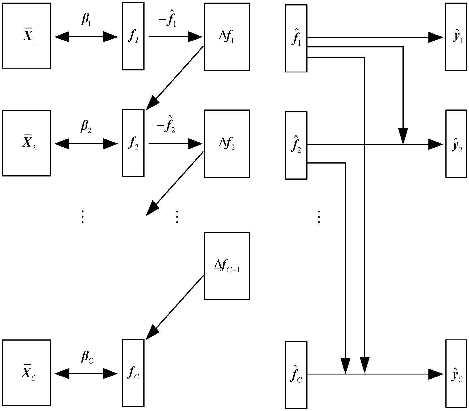
2.3. Multi-Phase Residual Recursive Modeling for Single Mode

In the phase-based PLS method, a phase regression model is established between the process variables and the final quality variables in each phase. It is assumed that in each phase, the model can capture the relationship between process variables and final quality variables. However, these individual models are not related to each other, and each phase seems to contribute to the final quality individually. This is in contradiction with the nature of the multi-phase batch process; that is, multi-phase acts on the final quality together in sequence. In addition, it should be noted that in the multi-phase batch process, the former phase may affect the later phase and the final process quality. In the current phase of quality regression modeling, the influence of the previous phases should be considered. Therefore, a recursive quality regression method for the multi-phase batch process is proposed, which uses the quality residuals of the previous phase model to establish the current phase regression model. All phases that are critical to quality are correlated by phase-based recursive regression residuals so that they together contribute to the final quality.

The establishment of a multi-phase residual recursive model is shown in Figure 1.

For a single phase, each phase is modeled by the regression between the average variable matrix ${\overline{X}}_c$ and the current quality residual $f_c$, then the regression parameter ${\mathsf{\beta }}_c$ and the residual prediction quantity ${\widehat{f}}_c$ are obtained,

$$\begin{array}{l}{f}_c={\overline{X}}_c{\mathsf{\beta }}_c+f^{*}\\ {\widehat{f}}_c={\overline{X}}_c{\mathsf{\beta }}_c\end{array}$$

(13)

The quality residual in the first phase $f_1$ is the quality measurement itself. The residual of the second phase is the deviation between the prediction quality of the first phase and the residual of the first phase, and so on.

The current phase quality prediction results are the sum of the completed phase and the current phase quality residual prediction,

$${\widehat{y}}_c={\displaystyle \sum _{i=1}^c{\widehat{f}}_i},c=1,2,\dots ,C$$

(14)

The final online quality prediction results are as follows:

$${\widehat{y}}_k^{}=\{\begin{array}{l}{X}_{k,c_1}{\mathsf{\beta }}_1 k\in c_1\\ {\widehat{f}}_1+X_k{}_{,c_2}{\mathsf{\beta }}_2 k\in c_2\\ {\widehat{f}}_1+{\widehat{f}}_2+X_k{}_{,c_3}{\mathsf{\beta }}_3 k\in c_3\\ {\widehat{f}}_1+{\widehat{f}}_2+{\widehat{f}}_3+X_k{}_{,c_4}{\mathsf{\beta }}_4 k\in c_4\end{array}$$

(15)

where c₁,…, c₄ are four phases, respectively, and $X_{k,c_1}$,…, $X_{k,c_4}$ are the phase mean variable matrices.

The Hotelling-T² and SPE statistics for the current time k are:

$${\mathit{T}}_k{}^2=x_k{}^{\mathrm{T}}{R}_k{(\frac{T_k{}^{\mathrm{T}}{T}_k}{I-1})}^{-1}{R}_k{}^{\mathrm{T}}{x}_k$$

(16)

$$\mathit{S}\mathit{P}{\mathit{E}}_k={\Vert {\tilde{x}}_k\Vert }^2={\Vert (I_{J_x}-P_k{R}_k{}^{\mathrm{T}})x_k\Vert }^2$$

(17)

where ${\tilde{x}}_k$ is the residual vector at the current time.

The corresponding control limits are:

$${\mathit{\delta }}_{{\mathit{T}}_k{}^2}(\alpha )=\frac{H(I^2-1)}{I(I-H)}{\mathit{F}}_{k\alpha }(H,I-H)$$

(18)

$$\mathit{S}\mathit{P}{\mathit{E}}_k(\alpha )={\mathit{g}}_k{\mathit{\chi }}_{h,\alpha }^2$$

(19)

where ${\mathit{F}}_{k\alpha }(H,I-H)$ is the $\mathit{F}$ distribution with $\alpha$ confidence and $H$ and $I-H$ degrees of freedom, and $H$ is the number of retained latent variables; ${\mathit{g}}_k{\mathit{\chi }}_{h,\alpha }^2$ is the ${\mathit{\chi }}_{}^2$ distribution with the same confidence level of $\alpha$ and the proportional coefficient of ${\mathit{g}}_k=s/2\mu$; $h=2{\mu }^2/s$; and $\mu$ is the mean value of SPE; $s$ is the variance of SPE.

2.4. Between-Mode Modeling for Multiple Modes

The multi-phase problem has been addressed in the previous part; thus, in this part, the multi-mode problem is the key interesting issue. While it does not mean the multi-phase problem is not considered any longer and without a special statement, the methodology below is proposed based on the above multi-phase analysis.

To solve the multi-mode problem, the main idea is to extract the relationship between the historical modes and the new mode. This proposed model contains more modal information and can better predict and monitor multiple modes. The framework of this section is shown in Figure 2. The model is established not only based on the new mode but also on the historical modes in the modal library. Firstly, the process variables and quality variables in historical modes are regressed and analyzed using the single-mode model. Secondly, the new mode process variables are applied to those single-mode models of historical modes, and the assumed predicted qualities of the new mode are obtained. Then, the regression analysis is carried out on the assumed predicted qualities and the final actual quality, obtaining the between-mode model. Finally, by applying the between-mode model, the final prediction quality is obtained. The details of between-mode quality regression modeling are introduced as follows.

Within phase c, for the new mode with the normalized time-slice process variables, $X_{t,k}\left(I_t\times J_x\right)$, and the quality variable $y_t$, process variables are first applied to the regression models obtained from the historical modes to obtain the assumed quality predictions,

$${\widehat{y}}_{t,m,k}=X_{t,k}{\mathsf{\beta }}_{m,c}$$

(20)

where m is the number of the historical modes, m = 1,2,…,M, and t represents the new mode. ${\widehat{y}}_{t,m,k}$ are the assumed prediction quality. ${\mathsf{\beta }}_{m,c}$ are the regression parameters of mode m of phase c for the historical modes. By obtaining the assumed quality predictions, the quality information of historical modes is shared by the new mode. Further, the quality information of historical modes will be judged and extracted by the next regression.

Then, the assumed quality predictions will be regressed with the quality data of the new mode. All these assumed predictions of the historical modes can comprise a new matrix $Z_{t,k}\left(I_t\times M\right)$, $Z_{t,k}=\left[{\widehat{y}}_{t,1,k},\dots ,{\widehat{y}}_{t,m,k},\dots ,{\widehat{\mathrm{y}}}_{t,M,k}\right]$. Then, the kth time-slice PLS regression model is built between $Z_{t,k}$ and $y_t$ as follows [29]:

$$\begin{array}{l}{Z}_{t,k}=T_{t,k}{P}_{t,k}^{\mathrm{T}}+E_{t,k}\\ y_t=U_{t,k}{Q}_{t,k}^{\mathrm{T}}+F_{t,k}\end{array}$$

(21)

where $T_{t,k}$ and $U_{t,k}$ are the score matrices of the new mode, $P_{t,k}$ and $Q_{t,k}$ are the loading matrices of the new mode, and $E_{t,k}$ and $F_{t,k}$ are the residual matrices of the new mode. Novel predictions are obtained,

$${\widehat{y}}_{t,k}^{*}=Z_{t,k}{\alpha }_{t,k}$$

(22)

where ${\widehat{y}}_{t,k}^{*}$ shows this new regression relationship of the between-mode relationship analysis, k = 1,2,…,K_c, and ${\alpha }_{t,k}$ is the regression parameter of the kth time-slice model.

The regression parameters of phase c can be obtained from the regression parameters of the time-slice model,

$${\alpha }_{t,c}=\frac{1}{K_c}{\displaystyle \sum _{k=1}^{K_c}{\alpha }_{t,k}}$$

(23)

where K_c is the number of the time intervals within phase c. Then the predictions, ${\widehat{y}}_{t,c,k}^{*}$, based on the regression parameter of the whole phase, ${\alpha }_{t,c}$, are obtained,

$${\widehat{y}}_{t,c,k}^{*}=Z_{t,k}{\alpha }_{t,c}$$

(24)

Then for phase c, corresponding coefficients can be obtained:

$$Z_{t,c}=\frac{1}{K_c}{\displaystyle \sum _{k=1}^{K_c}{Z}_{t,k}}$$

(25)

$$T_{t,c}=\frac{1}{K_c}{\displaystyle \sum _{k=1}^{K_c}{T}_{t,k}}$$

(26)

$$P_{t,c}=\frac{1}{K_c}{\displaystyle \sum _{k=1}^{K_c}{P}_{t,k}}$$

(27)

$$W_{t,c}=\frac{1}{K_c}{\displaystyle \sum _{k=1}^{K_c}{W}_{t,k}}$$

(28)

$$R_{t,c}=W_{t,c}{(P_{t,c}{W}_{t,c})}^{-1}$$

(29)

where $K_c$ is the number of time intervals in phase c, k = 1,2,…,K_c.

In online monitoring, the score matrix $T_{t,c}$, the load matrix $P_{t,c}$, and the weight matrix $W_{t,c}$ are obtained according to the offline model. The online T² statistics and online SPE statistics are calculated:

Online T² statistics:

$${\mathit{T}}_k{}^2=z_k{}^{\mathrm{T}}{R}_{t,c}{(\frac{T_{t,c}{}^{\mathrm{T}}{T}_{t,c}}{I-1})}^{-1}{R}_{t,c}{}^{\mathrm{T}}{z}_k$$

(30)

Online SPE statistics:

$$\mathit{S}\mathit{P}{\mathit{E}}_k={\Vert {\tilde{z}}_k\Vert }^2={\Vert (I_M-P_{t,c}{R}_{t,c}{}^{\mathrm{T}})z_k\Vert }^2$$

(31)

where ${\mathit{T}}_k{}^2$ and $\mathit{S}\mathit{P}{\mathit{E}}_k$ are the T² and SPE statistics calculated at the kth time interval, respectively, and ${\tilde{z}}_k$ is the residual vector of the kth time interval.

The corresponding control limits are:

$${\mathit{\delta }}_{T_k{}^2}(\alpha )=\frac{H(I^2-1)}{I(I-H)}{\mathit{F}}_{k\alpha }(H,I-H)$$

(32)

$$\mathit{S}\mathit{P}{\mathit{E}}_k(\alpha )={\mathit{g}}_k{\mathit{\chi }}_{h,\alpha }^2$$

(33)

where ${\mathit{F}}_{k\alpha }(H,I-H)$ is the F distribution with $\alpha$ confidence and $H$ and $I-H$ degrees of freedom, and $H$ is the number of retained latent variables; ${\mathit{g}}_k{\mathit{\chi }}_{h,\alpha }^2$ is the ${\mathit{\chi }}_{}^2$ distribution with the same confidence level of $\alpha$ and the proportional coefficient of ${\mathit{g}}_k=s/2\mu$; $h=2{\mu }^2/s$;$\mu$ is the mean value of SPE; and $s$ is the variance of SPE.

2.5. Model Comparison and Selection

In this section, two models are compared, which are the single-mode model and the between-mode model. To be clear, the single-mode model is introduced in Section 2.3. This model only considers one mode, and the quality is forecasted and monitored in its own mode on the basis of the critical-to-quality phase residual recursive analysis. The other model is developed in Section 2.4, and the between-mode model, which is established based on the historical modes and the new mode to obtain the assumed quality predictions and involve the quality information of the historical modes in the regression model for the new mode. It should be noticed that in both models, the multi-phase issue is addressed in the same way, by the residual recursive modeling, for the fair comparison as well as strategy consistency.

First, for the new batches $X_{new}\left(I_{new}\times J_x\right)$, the single-mode quality predictions ${\widehat{y}}_{new,t,m,k}$ are gained at kth time. The multi-mode quality predictions ${\widehat{y}}_{new,t,c,k}^{*}$ are gained at kth time.

$$\begin{array}{l}{\widehat{y}}_{new,t,c,k}=X_{new}{\mathsf{\beta }}_{t,c}\\ {\widehat{y}}_{new,t,m,k}=X_{new}{\mathsf{\beta }}_{m,c}\end{array}$$

(34)

$$\begin{array}{l}{Z}_{new,t,k}=[{\widehat{y}}_{new,t,1,k},\dots ,{\widehat{y}}_{new,t,m,k},\dots ,{\widehat{y}}_{new,t,M,k}]\\ {\widehat{y}}_{new,t,c,k}^{*}=Z_{new,t,k}{\alpha }_{t,c}\end{array}$$

(35)

Then, the root-mean-square error (RMSE) values are obtained,

$$RMSE=\sqrt{\frac{1}{I_{new}}{\displaystyle \sum _{i=1}^{I_{new}}{(y_{new,t,i}-{\widehat{y}}_{new,t,i,k})}^2}}$$

(36)

$$RMSE=\sqrt{\frac{1}{I_{new}}{\displaystyle \sum _{i=1}^{I_{new}}{(y_{new,t,i}-{\widehat{y}}_{new,t,i,k}^{*})}^2}}$$

(37)

The RMSE values can well reflect the precision of prediction. The smaller the RMSE values, the higher the prediction accuracy.

3. Illustration and Discussions

3.1. Process Description

Injection molding technology is one of the important means of plastic processing, and it is also a typical batch process. In order to accurately predict the quality of products, it is necessary to know enough about the injection molding process. A complete injection molding process is mainly composed of mold closing, injection, packing-holding, plasticizing, cooling, mold opening, part ejection, and other processes. There are four phases that are the most important operation phases to determine the quality of parts: the first one is the injection phase, which injects the molten plastic into the mold; secondly, in the packing-holding phase, the packaging materials are used under a certain pressure; then, in the plasticizing phase, the material is transported forward, plasticized and melted, and then transferred to viscous fluid for storage; the final phase is the cooling phase, where the plastic is cooled in the mold until the part becomes sufficiently rigid for ejection. The process variables that have an important influence on the final quality can be read online by high-precision sensors.

In this work, high-density polyethylene (HDPE) was used as the injection material. The quality index analyzed in this experiment is the weight of injection molded parts. According to the different settings of packing pressure (PP) and barrel temperature (BT), the experimental batches can be divided into five different modes. The experimental conditions are shown in

Table 1. Different operation modes.

Modes	PP/Bar	BT/°C
Mode 1	25	180
Mode 2	35	180
Mode 3	25	200
Mode 4	30	200
Mode 5	35	200

. The process data of each mode is stored in X (23 × 11 × 525). The quality data of each mode is stored in y (23 × 1). The data used in the modeling process are all real data obtained from experiments.

3.2. Critical-to-Quality Phase Identification

In the injection molding process, different phases have different effects on the quality of products. For example, in the injection phase, the main variables affecting the final product weight are the injection speed and the barrel temperature. In general, the higher the barrel temperature is, the lower the product weight is. The faster the injection rate increases, the more melt injection and the greater the product weight. In addition, the pressure variables (such as the nozzle pressure, the cylinder pressure), the screw stroke, the injection speed, and the barrel temperature are positively correlated with the sputtering quality of injection products. That is to say, the faster the injection speed, the higher the pressure and the temperature are, and the more likely the sputtering phenomenon will appear in the intermittent operation. In the packing-holding phase, the weight of the injection molded part is mainly determined by the nozzle pressure, the cylinder pressure, and the cavity pressure. Two temperature variables, the cavity temperature and the barrel temperature, also affect the weight of the product. The lower the temperature, the greater the weight.

Taking mode 3 as an example, the critical-to-quality phase analysis is carried out. There are 23 batches in mode 3. A total of 18 train batches are selected as the prediction batches to analyze the phase characteristics. The $R_k^2$ and the phase mean of $R_k^2$ are shown in Figure 3. It can be seen from the figure that the $R_k^2$ values of the injection phase and the packing-holding phase are larger, which means these two phases have greater impacts on the final prediction quality than other phases.

The phase mean value of $R_k^2$ of the four phases under three different modes is shown in

Table 2. Phase mean value $R_k^2$ of the different modes and different phases.

Phases	Mode 1	Mode 2	Mode 3	Mode 4	Mode 5	Mean
Injection phase	0.4567	0.7867	0.7161	0.8219	0.7643	0.7091
Packing-holding phase	0.4013	0.7500	0.6836	0.8234	0.7801	0.6877
Plasticizing phase	0.3893	0.7175	0.6214	0.8058	0.7839	0.6636
Cooling phase	0.3407	0.6415	0.5510	0.8002	0.8075	0.6282

.

According to the data in the above table, for mode 1, mode 2, mode 3, and mode 4, the phase mean values of $R_k^2$ of the injection phase and the packing-holding phase are greater than the phase mean values of $R_k^2$ of the plasticizing phase and the cooling phase. For mode 5, the phase mean value of $R_k^2$ of the cooling phase is the largest. Based on the mean $R_k^2$, the injection phase and the packing-holding phase are selected as the critical-to-quality phases for subsequent monitoring and analysis.

3.3. Multi-Phase Monitoring for Single Mode

In this part, the single-mode model is adopted for quality prediction and process monitoring. The first 18 batches of mode 3 are selected for modeling, and the last 5 batches of mode 3 are tested. According to the four-fold cross-validation method, in the modeling of the injection molding phase, the number of reserved latent variables of the traditional method and the proposed method is four. In the packing-holding phase, the number of latent variables of the traditional method is three, while the number of latent variables of the proposed method is two. The confidence level of $\alpha$ is set to 0.99. The simulation result of the predicted quality of one test batch is shown in Figure 4 and compared with the traditional partial multi-phase least squares method [30], in which for each phase, one single model is built for quality prediction. The mean RMSE predicted for the five test batches under different prediction methods are shown in

Table 3. RMSE of the different prediction modes in single-mode prediction.

Prediction Modes	Mode 3	Mode 1
Traditional method	0.0702	0.1398
Proposed method	0.0632	0.1154

. It can be seen from Table 3 that the mean RMSE predicted by the traditional method is 0.0702, while the mean RMSE predicted by the proposed method is 0.0632, which indicates that the proposed recursive method of phase residuals shows a more accurate prediction effect. The results of monitoring of the first test batch are shown in Figure 5 and Figure 6. Because the traditional method also divides the batch process into four phases, in each phase, the quality is directly predicted and monitored, and in the first phase the proposed method regards the actual quality as the residual of the first phase, so the prediction and monitoring effects of the first phase, namely the injection phase, of the traditional method and proposed method is the same. The monitoring results of the injection phase are shown in Figure 5. It can be seen that T² and SPE are not beyond the control limits. In Figure 6, the monitoring results of the packing-holding phase are shown. It can be seen that T² and SPE of both the traditional method and the proposed method are not beyond their respective control limits. This shows that the proposed modeling method based on a single mode can monitor the corresponding test batches.

In addition, batches from mode 1 are tested using the monitoring model built based on mode 3; that is, the first 18 batches of mode 3 are selected for modeling, and 5 batches of mode 1 are tested. The results of each phase of one batch of five test batches in mode 1 are displayed. The quality prediction result is shown in Figure 7 and compared with that of the traditional partial least squares method. The mean RMSE predicted for the five test batches under different prediction methods are shown in Table 3. The mean RMSE predicted by the traditional method is 0.1398, while the mean RMSE predicted by the proposed method is 0.1154, which indicates that the proposed recursive method of phase residuals shows a more accurate prediction effect. The monitoring results of the injection phase of mode 1 are shown in Figure 8. It can be seen that T² statistics do not exceed the control limit, but SPE statistics have exceeded the limit. The monitoring results of mode 1 in the packing-holding phase are shown in Figure 9. It can be seen that SPE statistics of the proposed method have exceeded the control limits in the beginning part. However, SPE statistics of the traditional method do not exceed the control limit. So the proposed method can distinguish this batch of mode 1 and is better than the traditional method. Thus, when a single mode is used for modeling, the other modes can be distinguished by the proposed method.

In order to compare the prediction effect of different modes and different methods under the single-mode modeling, RMSE of prediction results of five test batches of mode 3 and mode 1 are calculated respectively on the basis of the model of mode 3, as shown in Table 3.

It can be seen from the above table that in the single-mode modeling and prediction, the prediction effect of the test mode, which is the same as the modeling mode, is better than that of other test modes. In addition, according to the comparison of different methods, it can be concluded that the prediction effect of the proposed method is more accurate than that of the traditional method.

In the injection molding process, there are two main faults. One is material disturbance. A small amount of polypropylene (PP) is mixed into the original material HDPE. Because the viscosity of PP is higher than that of HDPE, higher heat will be generated in the operation process, resulting in the melt temperature in the nozzle being higher than the normal state. The second is the sensor fault. Due to the sensor fault, no data can be detected, resulting in a fault in the process.

First, a faulty batch caused by material disturbance is selected for monitoring, where the temperature variable is increased by 5 °C at the 60th sampling point. Therefore, according to the actual process situation, a batch is selected in the test batch of mode 3, and the temperature variable is increased by 5 °C at the 60th sampling point. The monitoring effects of the traditional method and the proposed method are shown in Figure 10. Compared with the traditional method, the monitoring effect of the proposed method is better since the statistics will rise rapidly when the fault occurs, especially for the T² statistics.

For the sensor fault, a test batch with the pressure variable removed after the 150th sampling point is monitored. The T² and SPE monitoring effects of the traditional method and the proposed method of the single-mode model are shown in Figure 11. Compared with the traditional method, the statistics of the proposed method rise more rapidly, and the amplitudes are relatively large.

3.4. Multi-Mode Monitoring

For the between-mode modeling analysis, 18 batches in mode 1, mode 2, mode 4, and mode 5 are selected respectively as historical modes. Mode 3 with 18 batches is used as the new mode for modeling. The test data are constructed by the five test batches of mode 3. According to the four-fold cross-validation method, in each phase of modeling, the number of reserved latent variables of the traditional method and the proposed method is two. The confidence level of $\alpha$ is set to 0.99.

In order to illustrate the advantages of the method proposed in this paper, it is compared with the traditional multi-mode and multi-phase methods, in which individual models are built for a single phase within a single mode. One batch of five test batches in mode 3 is selected to show the results. The simulation results of the prediction are shown in Figure 12. The mean RMSE predicted for the five test batches under different prediction methods are shown in

Table 4. RMSE of different prediction method.

Prediction Model	Prediction Method	Mode 3	Mode 1
Single-mode model	Traditional method	0.0702	0.1398
	Proposed method	0.0632	0.1154
Between-mode model	Traditional method	0.0496	0.1010
	Proposed method	0.0458	0.0876

. The mean RMSE predicted of mode 3 by the traditional method is 0.0496, while the mean RMSE predicted by the proposed method is 0.0458, which indicates that the proposed method shows a more accurate prediction effect. The monitoring results of the injection phase and the packing-holding phase of the first test batch of mode 3 are shown in Figure 13 and Figure 14, respectively. In Figure 13, it can be seen that T² and SPE do not exceed the control limits in the injection phase. In Figure 14, in the packing-holding phase, T² and SPE do not exceed their respective control limits.

In addition, in order to illustrate the monitoring of new test modes by the multi-phase multi-mode model, 18 batches of mode 2, mode 3, mode 4, and mode 5 are selected respectively as the historical modes for each phase, and the historical regression parameters are obtained. Mode 3 with 18 batches is used as the new mode for modeling to predict and monitor the new test batches of mode 1. The results of each phase of one batch of five test batches in mode 1 are displayed. The simulation results of quality prediction are shown in Figure 15. The mean RMSE predicted of mode 1 for the five test batches under different prediction methods are shown in Table 4. The mean RMSE predicted by the traditional method is 0.1010, while the mean RMSE predicted by the proposed method is 0.0876, which indicates that the proposed method shows a more accurate prediction effect. Figure 16 and Figure 17, respectively, show the monitoring results of the injection phase and the packing-holding phase of one test batch of mode 1. Because the historical mode and training data do not contain the information of mode 1, when monitoring, T² and SPE in the injection phase exceed the control limit, which will lead to an alarm.

In order to compare the prediction results of the single-mode model and the between-mode model of different prediction methods, RMSE values of five test batches in mode 3 and mode 1 are used for judgment, as shown in Table 4.

According to the simulation results, it can be concluded that the between-mode model extracts the related information in the historical modes, so it contains more necessary information. It can be seen from Table 4 that the prediction results of the between-mode model are better than those of the single-mode model. Comparing the RMSE of the traditional method and the proposed method, it can be seen that the proposed method is more accurate for quality prediction. From the monitoring figures, it can be seen that if part of the mode information has been included in the modeling process, the statistics do not exceed the control limit, leading to a suitable monitoring effect. In contrast, if the modeling process does not contain the mode information, the statistics will exceed the control limits. To sum up, compared with single-mode modeling, the between-mode modeling contains more historical modal information, leading to better prediction, and can achieve the purpose of information selecting for monitoring. Therefore, for the current modes modeling, the between-mode modeling method can be selected.

For faulty batch monitoring using the between-mode modeling, the faulty batch data is consistent with the single-mode modeling faulty batch data. First, the faulty batch caused by material disturbance is monitored. The monitoring results of the traditional method and the proposed method are shown in Figure 18. Both the proposed method and the traditional method can detect the fault.

Secondly, the monitoring effects of the traditional method and the proposed method for the sensor fault are shown in Figure 19. Compared with the traditional method, the statistics of the proposed method rise more sharply, and the amplitudes are relatively large.

4. Conclusions

In this work, based on the analysis of multi-phase multi-mode batch processes, a combination of the multi-phase quality residual recursion model for multiple phases and the between-mode model for multiple modes is proposed, and according process-monitoring strategies based on quality analysis are developed. Firstly, the critical-to-quality phases are identified and selected based on the influence of different phases on the final quality of the batch process. Then, the phase mean model is established, and based on the multi-phase quality residual recursive model, the quality predictions of critical-to-quality phases are obtained, and those phases are monitored. On the other hand, the between-mode model is used to analyzes the regression relationship between the process variables and the quality of the new mode through the historical modes, and online monitoring is carried out on this basis. Through the simulation of the experimental data of an injection molding process, it is proved that due to better quality predictions, the proposed strategy can provide better process-monitoring results for multi-phase multi-mode batch processes.

However, the experimental data used in this paper are all processed so that the length of the same phase of different batches is equal, which is often difficult to achieve in the actual industry due to various reasons, such as the influence of climate, the quality difference of raw materials, the data acquisition system based on a non-time coordinate, etc. In order to solve this problem, the effect of this method on the data of the batch process with unequal data lengths should be considered. For this, further research will be conducted in the future.