Article

Numerical Simulation of Passive Cooling Beam and Its Optimization to Increase the Cooling Power

by
Katarína Kaduchová
and
Richard Lenhard
*
Department of Power Engineering, Faculty of Mechanical Engineering, University of Zilina, 010 26 Zilina, Slovakia
*
Author to whom correspondence should be addressed.
Processes 2021, 9(8), 1478; https://doi.org/10.3390/pr9081478
Submission received: 3 June 2021 / Revised: 12 August 2021 / Accepted: 20 August 2021 / Published: 23 August 2021
(This article belongs to the Special Issue Experimental and Numerical Methods in Fluid Mechanics and Energy)

Abstract

:
This article is focused on the research of passive cooling beams and increasing their cooling capacity. A passive cooling beam with four tubes was chosen as a model. A mathematical model was built using the corresponding criterion equations to capture the behavior of a passive cooling beam. This mathematical model can be used to optimize geometrical parameters (the distance between the ribs, rib height and thickness, and diameter and number of tubes), by changing these geometric parameters we can increase the cooling performance. The work includes a mathematical model for calculating the boundary layer, which has a significant influence on the cooling performance. The results obtained from the created mathematical model show that the model works correctly and can be used to optimize the cooling performance of passive cooling beams. To better understand the behavior of a passive cooling beam in a confined space, the entire device was numerically simulated, as was the flow in the intercostal space.

1. Introduction

Thermal comfort is one of the most important phenomena of an environment for well-being, such as well-being at work and, thus, the performance of people at work. By an environment that facilitates well-being, we mean an environment in which the environmental factors that affect a healthy person at a given moment are so balanced that the person is not aware of their effects [1,2]. An optimal temperature of 22 ± 2 °C is assumed for our Central European climate for a normally dressed, seated person who does not perform any physical work. The use of ceiling cooling convectors not only ensures optimal thermal comfort, but also contributes to reducing the energy use of buildings [3].
Thermal comfort can, therefore, be achieved at different air temperatures and corresponding internal surface temperatures. Establishing an optimal indoor climate requires applying ti-tip ≤ 2 °C (ti is the indoor air temperature (°C); tip is the surface temperature of the internal surfaces (°C)). For ceiling cooling, therefore, the indoor room air temperature can be 1 to 3 K higher than that with conventional air conditioners while maintaining the same feeling of thermal comfort.
Passive ceiling cooling systems are a very good technology for space cooling in buildings. These systems handle the sensitive load by mostly cooling through natural convection and radiation from the ceiling level in the room, while the latent load is addressed separately by means of a parallel ventilation system. Although beam-type [4,5,6,7] and embedded-type ceiling cooling systems [8,9,10,11] have been studied extensively, there are not enough studies related to passive cooling beams and the optimization of their geometry.
To design passive cooling convectors, it is necessary to determine their cooling capacity, which is given for the temperature drop of cooling water to 16/19 °C or 16/18 °C. However, the cooling output depends not only on the temperature drop of cooling water but also on the temperature drop between the mean cooling water temperature and the ambient temperature, Dt. Such a problem is addressed in this work, as in [12], in which the effect of thermal load on the performance of a cooling convector was simulated.
This research mainly addressed the issue of optimizing the design parameters of ceiling passive cooling convectors with respect to maximizing the cooling capacity. For similar designs of passive ceiling cooling beams from different manufacturers [13,14,15,16], analysis was performed in terms of their specific power per meter of convector length. In order to optimize the design parameters of cooling convectors, it was necessary to theoretically describe the heat transport, which consists of heat transfer from water to the pipe, heat conduction through the pipe, and fin and heat transfer from the fin and pipe to the environment. On the basis of this theory, a model for the vertical flow around the plate was created, and based on this theory, a model was created to simulate the cooling power for the passive cooling ceiling convector. Simulation programs were created from the aforementioned models, on the basis of which the effects of various design parameters on the cooling capacity of passive ceiling cooling convectors were analyzed. A flow-around vertical rib was also simulated using computational fluid dynamics (CFD) methods in the program Fluent [17].
Using the created mathematical model of the passive ceiling cooling convector, simulations were performed for various changes in the design parameters of the passive cooling convector. The simulations were performed under conditions of constant length and width for the passive cooling convector with any change in design parameters. Based on the simulation calculations, it was determined how changes in fin spacing, fin height, fin thickness, tube diameter and the number of tubes affected the cooling capacity.

1.1. Governing Equations

A passive cooling beam is actually a rib pipe heat exchanger in which cooling water runs. The convector is set under the roof, but the length must be at least half of the width of the convector. Warm air is cooled in the top part of the convector and then naturally falls through the convector.
Today, cooling convectors show relatively low cooling power due to their lengths, necessitating an increase in their cooling power through adjustments to their structure or by selecting appropriate temperature gradients or variations in the flow of coolant, thereby increasing the cooling power without modifying the structure.
The movement of air is caused by a change in its density and the resulting temperature changes in the flow. Natural convection flow can be laminar or turbulent, as shown in Figure 1, which shows laminar and turbulent convection off a boundary layer of a vertical plate [3,18]. The cooling performance is dependent on the temperature gradient between the mean temperature of the cooling water and ambient temperature, and especially the geometry, particularly the spacing of the ribs. The spacing of the ribs is dependent on the size of the boundary layer of the natural flow of the convector rib; the spacing of the ribs should not influence the boundary layers. Passive cooling beams often show poor performance due to their layout length, because optimization is performed using mathematical simulations.

1.2. Mathematical Model of Passive Cooling Beam

  • Geometric parameters: the width, length, inner diameter of the pipe, outside diameter of the pipe, height of the ribs, thickness of the ribs, and spacing of the ribs;
  • Calculation of the required exchange surface for the heat exchanger: surface ribs and pipes.
Surface ribs and pipes [2,19,20,21]:
The inner surface of the pipe of the relevant section:
S 1 = π · d 1 · s r [ m 2 ]
sr—the spacing of the ribs (m); d1—the inner diameter of the pipe (m); d2—the outside diameter of the pipe (m).
The entire inner surface area of the pipe:
S 1 = L k · n r u r s r · S 1 [ m 2 ]
The surface area of all the free pipes for the section:
S r u r = π · d 2 · ( s r σ r ) · n r u r · n r [ m 2 ]
σr—the thickness of the ribs (m); nrur—number of pipes (pcs); nr—number of ribs (pcs).
The outer surface area of all the ribs:
S r = [ B · h r ( π · d 2 2 4 · n r u r · 2 ) ] · n r [ m 2 ]
B—the width of the rib (m).
The entire external surface area:
S 2 = S r + S r u r [ m 2 ]
  • Selection of the coolant: interior temperature, 26 °C; cooling water temperature, 16 °C;
  • Finding the physical properties of the liquids: ρ, c, ν and λ.
    The physical properties of the fluids are determined, and the temperature is changed, using, where appropriate, a function of the temperature.
  • The choice of the flow rate in the heat exchanger: vv.
The rate of the flow of water is set such as to achieve the desired thermal gradient of 16/19 °C.
The water velocity in the pipes:
v v = m v 3600 · S p · ρ [ m · s 1 ]
vv—the flow velocity in the pipe (m.s−1); Sp—the flow in the cross section (m2); S2—the size of the heat transfer surfaces of the heat exchanger (m2).
  • Determination of the heat transfer coefficient: α.
The heat transfer coefficient on the side of the water is a factor dependent on the flow rate and temperature of the water. It is possible to set it according to the following equation.
α i = 2900 · m v · 0.99 · ( 1 + 0.014 · t 11 ) [ W · m 2 · K 1 ]
The heat transfer coefficient for a passive cooling beam in natural flow determines the Prandtl and Grashof criteria, which are determined by Elenbaas semi-empirical correlation Nusselt numbers for isothermal parallel plates with spaced at sr [2,19,21] and from the size of the Rayleigh criteria-number:
R a s r = g · β · ( T 11 T 21 ) · s r 3 υ · a · S 1 ´
N u s r = 1 24 R a s r ( s r L ) { 1 exp [ 35 R a s r ( s r / L ) ] } 3 / 4
Substitution provides the heat transfer coefficient on the rib:
Nu = α r · h r λ α r = Nu · λ h r
hr—the height of the ribs (m).
The heat transfer coefficient on the outside of the pipe is determined using the following equation:
α e = α r · ψ [ 1 + ( η 1 ) · S r S 2 ] [ W · m 2 · K 1 ]
Efficiency of rib, η:
Since the temperature of the surface of a finned pipe is not the same, an adjustment factor ψ is necessary; for square ribs, ψ = 0.85. The efficiency of the rib is denoted by η [2,19,21].
  • The efficiency at the middle logarithmic temperature difference is determined:
The efficiency at the middle logarithmic temperature difference is determined based on the knowledge of the input and output temperatures of both substances.
Δ t str = ς ( t 21 t 12 ) ( t 22 t 11 ) ln t 21 t 12 t 22 t 11 [ ° C ]
t11—the inlet water temperature (°C); t12—the outlet water temperature (°C); t21—the temperature of the cooling air (°C); t22—the cooled air temperature (°C); Δtstr—the middle logarithmic temperature difference (°C).
Correction   factor   ς = ln 1 P 1 RP n · ( 1 R ) · ln [ 1 + 1 R · ln R 1 R ( 1 P 1 R · P ) 1 n 1 ]
P = t 12 t 11 t 21 t 11 R = t 12 t 22 t 12 t 11
  • Calculation of the heat transfer coefficient: k.
The heat transfer coefficient is calculated based on the partial heat transfer coefficients:
k = 1 1 α e + S 2 S 1 · 1 α i [ W · m 2 · K 1 ]
S1—the inner surface area of the pipe (m2); αi—the heat transfer coefficient on the inside (W·m−2·K−1); αe—the heat transfer coefficient on the outside (W·m−2·K−1); k—the thermal conductivity coefficient (W·m−2·K−1).
  • Determination of heat flux: Q.
Q = k · S 2 · Δ t str [ W ]
The aim of the simulation calculations was to analyze the impact of structural parameters on the cooling power of the passive cooling beam.
  • The passive cooling beam has the following design parameters:
d1—the outer pipe diameter, 0.015 m; sr—0.005 m, the spacing of the ribs; hr—the rib height, 0.06 m; σr—the rib thickness, 0.00025 m; Lk—the length of the passive ceiling convector, 1.8 m; B—the width of the passive ceiling convector, 0.6 m; nrur—the number of tubes, 4.

2. The Results of Simulations When Changing the Spacing of the Ribs, Sr

The simulations for changing the spacing of the ribs kept all the design parameters (the length, width, pipe diameter, rib height, rib thickness and number of tubes) constant; only the spacing between the ribs was varied, from 1 to 10 mm (Figure 2). Changing the spacing of the ribs from the original 5 mm to 8 mm increased the power to 107 W, which is the maximum possible cooling power with a change in rib spacing.

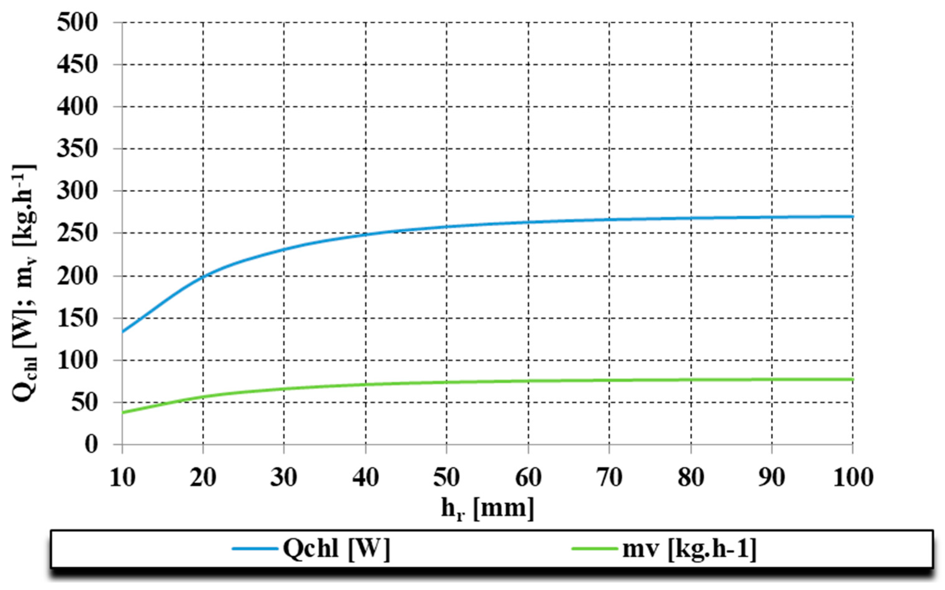
2.1. Simulation Results When Changing the Height of the Ribs, hr

Most of the parameters were kept constant in these simulations (the length, width, pipe diameter, spacing of the ribs, rib thickness and number of tubes); only the height of the ribs was changed, from 10 to 100 mm (Figure 3). Changing the height of the ribs from 50 to 100 mm resulted in a cooling power of 269.89 W, which is the maximum possible cooling power from altering the height of the ribs. We observed that the increase in cooling power achieved by increasing the rib height to 60 mm was negligible.

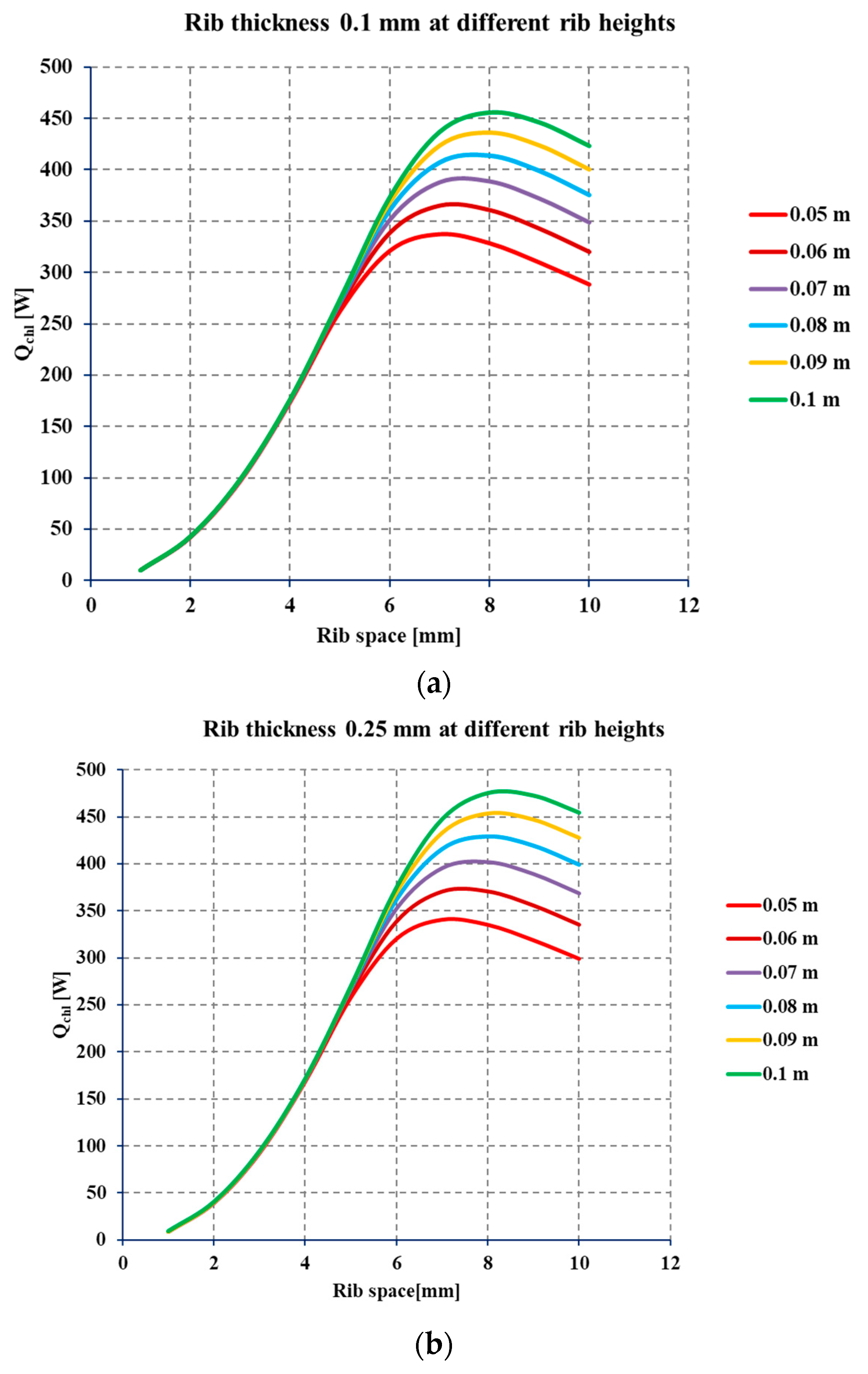
2.2. Results of the Simulation When Changing the Spacing of the Ribs and the Height of the Ribs at a Given Thickness of the Rib

The simulation results (Figure 4a–c) show that the cooling power depends on the passive cooling beam in terms of both the rib spacing and the heights of the ribs. The optimal rib spacing for maximizing the cooling power depends on the height; for example, at a rib height of 50 mm, the maximum cooling capacity of 320 W is achieved with 7 mm rib spacing, while at a rib height of 100 mm, the maximum cooling capacity of 475 W is achieved with 8 mm rib spacing. This must be considered in the construction of passive cooling beams.

Simulation Results When Changing the Number of Tubes

Optimization with respect to other parameters was performed, investigating the influence of the number of tubes on the cooling power and the final weight of the convector. The maximum cooling power of 532.58 W was achieved with equipment weighing 26.08 kg, having already taken into account the previous optimization (Figure 5).
The simulations showed that the cooling power increased with the number of tubes, but as the number of tubes increased from 14 to 20, the effect on the cooling power was negligible. This increase would impact the weight and, hence, the cost of production. Based on these simulations, it is recommended to implement passive cooling beams with the following design parameters: optimal performance: 517.79 W; number of tubes: 14 pcs; rib height: 0.1 m; rib length: 0.6 m; pitch: 8 mm; rib thickness: 0.3 mm; and weight: 21.41 kg.

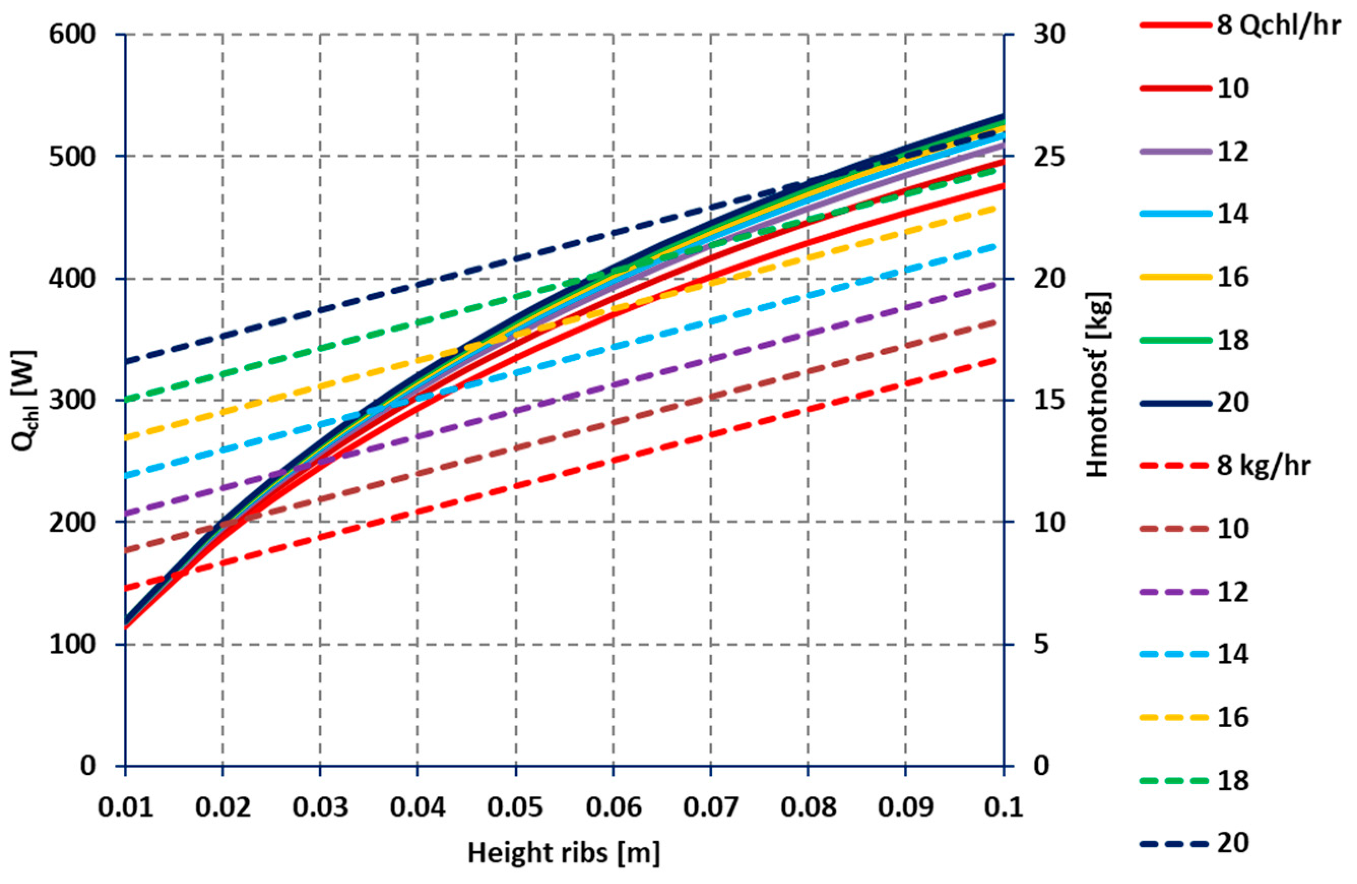
3. Increasing the Cooling Power of the Passive Cooling Beam with Change in Temperature Gradient and Change in Coolant Flow

The cooling power changed in response to a change in the rate of flow of the coolant (Figure 6).
Result of simulations comparing the percentage change in power with the change in flow for the temperature drop and the flow at which the cooling power of the convector was measured and the percentage change in cooling power related to the maximum power at flow 0.06 kg/s (Table 1).

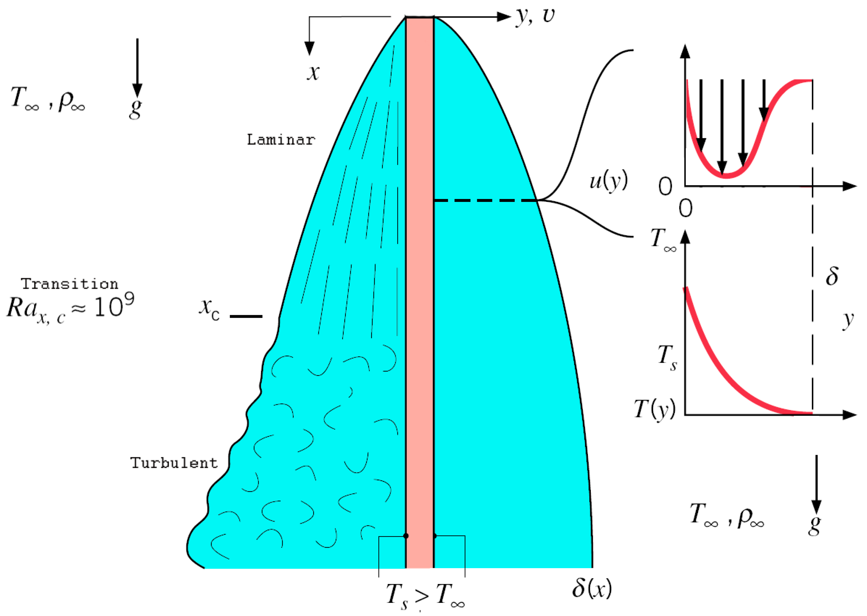
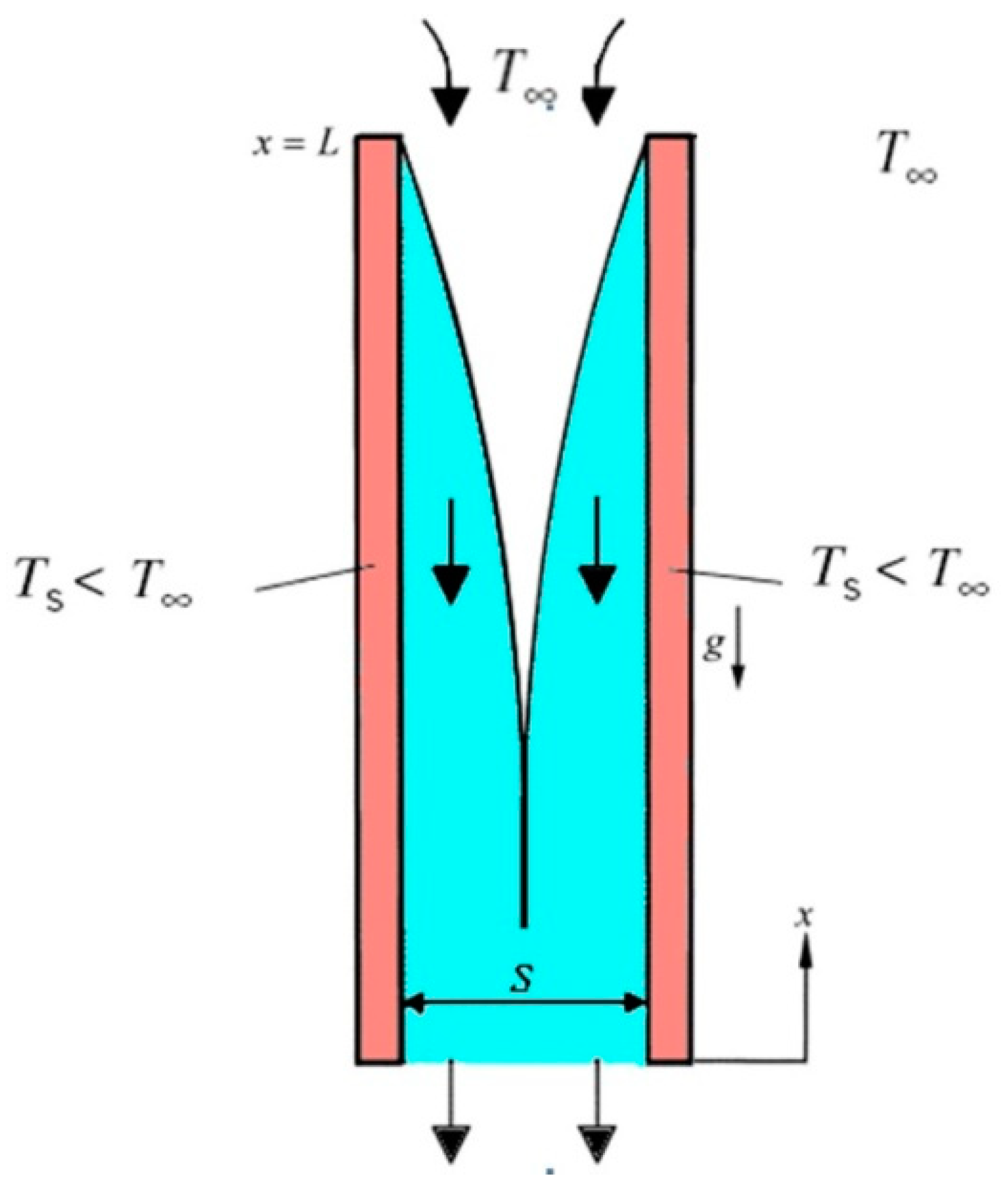
4. Model of the Boundary Layer for Rib Established through Differential Equations Describing Natural Convection

Based on the optimization of the spacing of the ribs for the passive cooling beam ceiling in relation to the boundary layer, it is necessary to establish a mathematical model. The development of the model is based on 2D flow, as shown in Figure 1. It is based on the momentum Equation (16), which is the same as for 2D flow between the layers and the volume expansion factors β [3,17,19,21,22].
u u x + v u y = 1 ρ p x g + v 2 u y 2
If there is no fluid movement in the direction y, the pressure gradient ∂p/∂y = 0. Therefore, the gradient ∂p/∂x must be the same in the boundary layer marginal layer on the outside. Assuming that the density varies linearly only with temperature and is independent of pressure (this simplification is described in the literature as the Boussinesq approximation), the momentum Equation (16) gives the resulting shape after treatment:
u u x + v u y = g β ( T T ) + v 2 u y 2
By introducing criterion similarities in Equation (17) and the treatment, we obtain the following criterion of similarity, called the Grashof criterion (18), which is a typical criterion for natural convection.
g β ( T T ) L u 2 u 2 L 2 v 2 Re 2 = g β ( T T ) L 3 v 2 Gr L
The characteristic dimension L is the amount of rib where there is air movement. The equation for determining the heat transfer coefficient is the Nusselt criterion and has the form:
N UL = f · ( G r L · P r )
GrL · Pr is known as the Rayleigh criterion. In natural convection, laminar or turbulent regimes are encountered. The criterion for determining the type of flow is the critical value of the local Rayleigh criteria:
Ra x , krit = Gr x , krit · Pr = g β ( T w T ) x 3 va = 10 9
For vertical surfaces, if Rax > 109, the flow regime is turbulent, whereas if Rax < 109, the regime is laminar. For a vertical wall—in this case, the vertical ribs of the passive cooling beam—the following equation for the local heat transfer coefficient on the along plate can be used:
α x = 0.508 Pr 1 / 2 Gr x 1 / 4 ( 0.952 + Pr ) 1 / 4 λ x
Equation (22) can be used to determine the boundary layer thickness:
δ x = 4.3 x [ Pr + 0.56 Pr 2 Gr x ] 1 / 4
where Grx is the local Grashof number, which is taken as the characteristic dimension of the x-axis position on the board. From the relation (21), it is clear that the heat transfer coefficient decreases by x1/4 with each integer increase in x, while the boundary layer thickness increases by x1/4. Equation (21) can be integrated for the walls, dividing the value of L obtained for the mean correlation coefficient of heat transfer, respectively. The Nusselt numbers for a laminar regime are as follows:
Nu ¯ L = α L ¯ λ = 0.678 Pr 1 / 2 Gr L 1 / 4 ( 0.952 + Pr ) 1 / 4

5. Results from Simulations

The cooling power of a passive cooling beam is considerably influenced by the spacing of the ribs. In relation to the boundary layer, it is necessary to choose a spacing of the ribs that avoids the connection of the two layers in the limited space. Figure 7 shows the dependence of the boundary layer thickness and average factors for heat transfer on the rib with a wall temperature tw = 16 °C at an ambient temperature = 25 °C, which is, in most cases, the required temperature for the cooling environment for measuring the passive cooling beam [23]. The results of the simulations are indicated in Figure 8 and Figure 9, where the behavior of the velocity and temperature profiles of the boundary layers depending on the rib height is shown. From these results, it is possible to determine the most appropriate structure for optimizing rib flow in passive ribbed cooling convectors and thus maximizing the cooling performance of a passive cooling beam.
For example, for a common design of passive convectors with a rib height of 0.06 m, a rib spacing of 5 mm and a rib wall temperature tw = 16 °C, Figure 7 shows that the boundary layer thickness is 3.27 mm. Similarly, for a rib wall temperature, tw to 18 °C, Figure 10 shows that the boundary layer thickness is 3.5 mm in both cases for the conflict boundary layers. For a passive cooling beam, the thickness of the boundary layer appears to be related to the rib spacing as it varies from 6 to 7 mm. Note that this does not consider other influences on the cooling power of the convector.

6. Natural Convection from Parallel Vertical Ribs

The beams are parallel cooling ribs with regular spacing. In terms of the intensification of heat transfer, it is necessary to know the arrangement of the ribs. Criterion equations characterize the free convection around spaced parallel ribs and the relationships that are important for the optimization of the spacing of the ribs with respect to the desired parameters for air. It follows that the boundary layer starts to develop on the leading edge of vertical plates if the thicknesses of the boundary layer growths of small and marginal layers are separated by air of the operational environment, but if the plates are long enough, or their spacing is small, then the boundary layers are combined to form a combined stream area (Figure 11). This means that, for the various geometrical shapes, the temperature of the ribs and various internal climate conditions influence the spacing of the ribs, sr. If the spacing is too small between the layers, both sides will interact, which will be reflected by increased hydraulic resistance. It may be such that the transmitted pitch reduces the heat output, which, because of the larger spacing, could be higher.
Elenbaas semi-empirical correlation Nusselt numbers for isothermal parallel plates with spacing, sr [19,21].
Nu s r = 1 24 Ra s r ( s r L ) { 1 exp [ 35 Ra s r ( s r / L ) ] } 3 / 4
Ra s r = g β ( T 11 T 21 ) s r 3 ν a

7. Numerical Modeling of Heat Transfer in Passive Cooling Beam

The heat transfer in the passive cooling beam was analyzed to compare the results of the mathematical simulations and the results obtained by CFD methods, as well as to visualize the behavior of the boundary layer in the intercostal space.

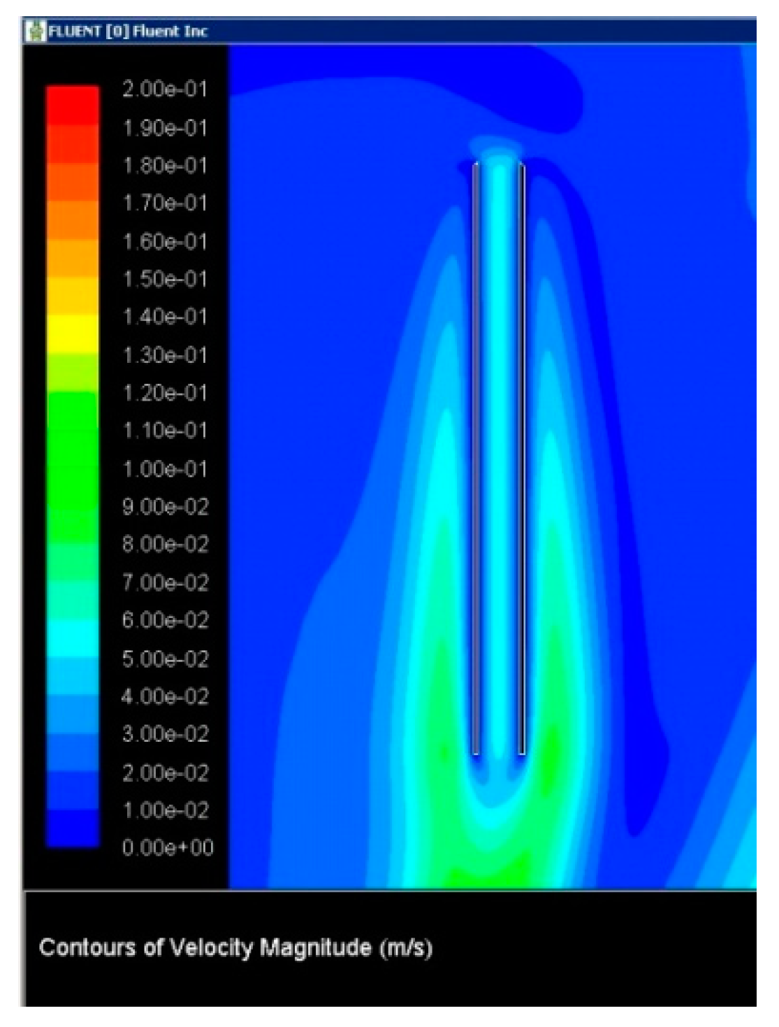
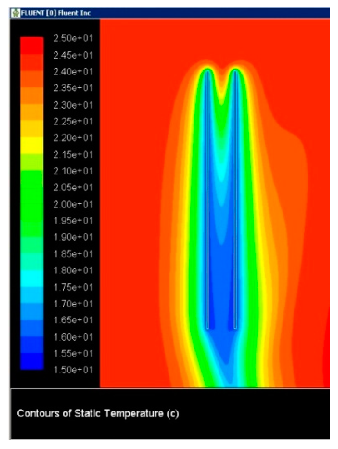
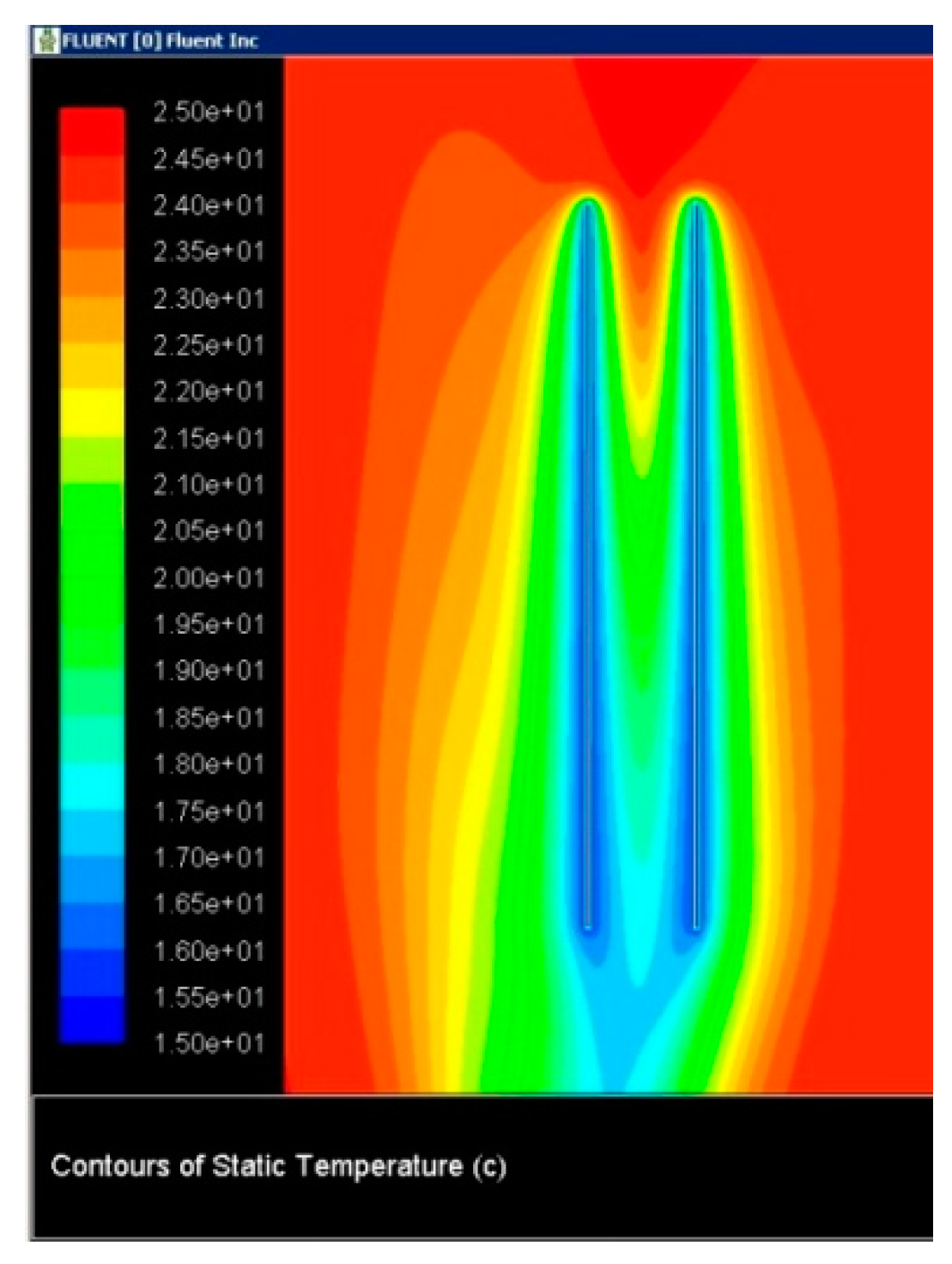
7.1. Modeling the Impact of the Height and Spacing of the Ribs, and the Cut-Off Layer in the Intercostal Space

A Gambit two-dimensional model of vertical plates (ribs) of heights 60, 70, 80 and 100 mm at intervals of 5, 7 and 10 mm was created. This model was exported form Gambit to the Fluent program, where boundary conditions corresponding to the calculations according to the criterial equations (plate temperature, 16 °C; gravitational acceleration, 9.81 m·s−2; ambient temperature, 25 °C) were set. A laminar flow model was entered, which was based on the calculation of Rayleigh numbers (Figure 12).

7.2. Analysis of the Results Obtained

In modeling the boundary layer in the intercostal space using CFD simulations, the goal was to determine the relationship between the layer and the behavior of the boundary layer when changing the spacing between the plates at different plate heights. Figure 13, Figure 14, Figure 15, Figure 16, Figure 17 and Figure 18 show the velocity and temperature fields of isothermal vertical plates in natural convection. In these figures, the velocity and temperature boundary layer are observable. Simulations for the resulting performance for each design were obtained (Table 2).
In achieving the optimal spacing for each plate, it is necessary to make the contact occurring on the layers as late as possible or prevent it completely. Conflict boundary layers have a significant effect on the cooling performance. If the spacing between the boundary layers is too small, they interact, and this reduces the cooling capacity; if the spacing increases, the cooling capacity can be increased. This is also observable in Table 2, which shows the cooling performance resulting from individual designs.
From the simulation results, we can conclude that the best spacing is 7 mm above plates with a height of 50 mm. This argument was also proved by the final results that were achieved in these simulations (Table 2). These spacings should be considered when optimizing a passive cooling beam.

7.3. Computational Fluid Dynamics (CFD) Simulation of Passive Cooling Beam in the Room

The Gambit program was used to model a cooling beam. This cooling beam was inserted into a control volume that simulated a room (Figure 19) and result is shown in Figure 20, Figure 21 and Figure 22 [17,24,25,26,27,28].
Input parameters:
For the input parameters, real structural dimensions of the devices were taken. In the modeling, it was necessary to take into account the complexity of the ribbing itself. Therefore, the space between the ribs was replaced with simulations of porosity. The whole model comprised about 5 million elements.
  • The viscous model was laminar (natural convection).
  • The inlet and outlet of the convector were taken to be the interior.
  • Aluminum rib: solid.
  • The water in the tubes: liquid and its temperature.
  • Copper pipe convector: wall thickness and heat transfer.
  • The thickness and temperature of the room walls have been set to prevent leakage ambient temperature: temperature-(adiabatic wall). The temperature of the walls of the room and thickness were set to avoid leakage to the surroundings: temperature—(adiabatic wall).
  • The acceleration of gravity, 9.81 m·s−1, was considered in the calculation.

8. Discussion and Conclusions

The resulting simulations were compared with the results of measurements of air flow and temperature for a passive cooling beam. For comparison, the temperature field of a thermovision and CFD model were analyzed to follow the conformity to cooling under a stream of air convectors where the temperature distribution had the same funnel shape. This correlation allowed us to conclude that CFD methods are appropriate means for modeling natural convection and the air flow behavior of the convector. It should be noted, however, that, for the simulation of entire passive cooling convectors, the real dimensions place high demands on computer performance.
The results of the mathematical simulations of the boundary layer in the intercostal space of a passive cooling beam show that the changes in rib spacing and rib height are affected by the layer, which affects the transport of heat from the cooling water to the environment and, thus, the overall cooling power of the passive cooling beam. The results of the simulations can be used to determine the optimal size and spacing of ribs to maximize the cooling performance of a passive cooling beam.
In the simulations of cooling power depending on the design parameters (the spacing of the ribs, rib height and thickness, and diameter and number of tubes), for a temperature gradient of 16/19 °C, it was found that the various parameters affected the cooling power of the passive cooling beam. The simulation results clearly show that changing the spacing of the ribs has the greatest effect on the cooling power.
In the simulations of the percentage change in the cooling power in response to variations in the flow rates for a given temperature gradient, it was found that better flow could be achieved by increasing the cooling power of the cooling convector. A similar dependence was calculated for a constant flow of coolant when changing the temperature gradient.

9. Limitations of the Work

From the results of the simulations, it is observed that the created mathematical model works with a certain deviation, which can be compensated for with a constant of 1.53 for ΔT = 7.5 K and 1.16 for ΔT = 8 K. The difference between the correction factors could be caused by various influences that cannot be included in the simulation calculation for passive ceiling cooling convectors. These include the influence of the room in which the convector is located, the position of the convector and the humidity in the room.

Author Contributions

Formal analysis, K.K.; Methodology, K.K.; Project administration, K.K.; Software, R.L.; Validation, R.L.; Writing—original draft, R.L. All authors have read and agreed to the published version of the manuscript.

Funding

This paper was written with financial support from the grant agency KEGA within the project solution No. 048ŽU-4/2019 and No. 046ŽU-4/2021 and supported by the Grant System of the University of Žilina No. 1/2020. (8024).

Institutional Review Board Statement

Not applicable.

Informed Consent Statement

Informed consent was obtained from all the subjects involved in this study.

Data Availability Statement

Not applicable.

Conflicts of Interest

The authors declare no conflict of interest.

Nomenclature

Nomenclature and related units for abbreviations.
Bwidth of passive ceiling convector (m)
cspecific heat capacity (J·kg−1·K−1)
d1inner diameter of the pipe (m)
d2outside diameter of the pipe (m)
ggravity (m·s−2)
GrGrashof’s number (-)
Grxlocal Grashof’s number (-)
Grx,kritcritical local Grashof’s number (-)
hrheight of the ribs (m)
kheat transfer coefficient (W·m−2·K−1)
Lklength of passive ceiling convector (m)
mvmass flow of water (kg·s−1)
mvzmass flow of air (kg·s−1)
nrnumber of ribs (pcs)
nrurnumber of pipes (pcs)
NuNusselt number (-)
PrPrandtl number (-)
Qheat flux (W)
Qchlcooling power (W)
RaRayleigh criterion (-)
ReReynolds number (-)
srspacing of the ribs (m)
Srouter surface of all the ribs (m2)
Srursection of all free pipes (m2)
Spflow cross section (m2)
S1inner surface area of pipe (m2)
S2size of the heat transfer surfaces of the heat exchanger (m2)
S′1the inner surface area of the tube of the section concerned (m2)
twwall temperature (°C)
t11inlet water temperature (°C)
t12outlet water temperature (°C)
t21temperature of the cooling air (°C)
t22air temperature cooled (°C)
Δtstrthe middle logarithmic temperature difference (°C)
ΔTtemperature difference (°C)
Tambient temperature (°C)
vvflow velocity in the pipe (m·s−1)
αheat transfer coefficient (W·m−2·K−1)
αeheat transfer coefficient on the outside (W·m−2·K−1)
αiheat transfer coefficient on the inside (W·m−2·K−1)
αrheat transfer coefficient on the rib (W·m−2·K−1)
αxaverage heat transfer coefficient at the rib height (W·m−2·K−1)
βcoefficient of volume expansion (1/K)
δboundary layer thickness (m)
ηefficiency of the rib (%)
λthermal conductivity coefficient (W·m−1·K−1)
υkinematic viscosity of the fluid (m2·s−1)
ρdensity (kg·m−3)
σrthickness of the ribs (m)
ψcorrection factor (-)
ςcorrection factor (-)

References

  1. Awbi, H.B. Ventilation of Buildings; Taylor & Francis e-Library: Abingdon, UK, 2003. [Google Scholar]
  2. Jícha, M. Přenos Tepla a Látky; Akademické Nakladatelství CERM: Brno, Czech Republic, 2001; Volume 160. [Google Scholar]
  3. Al-Waked, R.; Nasif, M.S.; Groenhout, N.; Partridge, L. Energy Performance and CO2 Emissions of HVAC Systems in Commercial Buildings. Buildings 2017, 7, 84. [Google Scholar] [CrossRef] [Green Version]
  4. Oosthuizen, P.H.; Taylor, D. An Introduction to Convective Heat Transfer Analysis; International Editions. William C Brown Pub., 1998; Volume 624. Available online: https://www.biblio.com/9780070482012 (accessed on 19 August 2021).
  5. Tian, Z.; Yin, X.; Ding, Y.; Zhang, C. Research on the actual cooling performance of ceiling radiant panel. Energy Build. 2012, 47, 636–642. [Google Scholar] [CrossRef]
  6. Okamoto, S.; Kitora, H.; Yamaguchi, H.; Oka, T. A simplified calculation method for estimating heat flux from ceiling radiant panels. Energy Build. 2010, 42, 29–33. [Google Scholar] [CrossRef]
  7. Tye-Gingras, M.; Gosselin, L. Comfort and energy consumption of hydronic heating radiant ceilings and walls based on CFD analysis. Build. Environ. 2012, 54, 1–13. [Google Scholar] [CrossRef]
  8. Koschenz, M.; Dorer, V. Interaction of an air system with concrete core conditioning. Energy Build. 1999, 30, 139–145. [Google Scholar] [CrossRef]
  9. Antonopoulos, K.A. Analytical and numerical heat transfer in cooling panels. Int. J. Heat Mass Transf. 1992, 35, 2777–2782. [Google Scholar] [CrossRef]
  10. Kim, J.; Tzempelikos, A.; Braun, J.E. Review of Modeling Approaches for Passive Radiant Ceiling Cooling Systems. J. Build. Perform. Simul. 2015, 8, 145–172. [Google Scholar] [CrossRef]
  11. Kim, J.; Tzempelikos, A.; Horton, W.T.; Braun, J.E. Experimental investigation and datadriven regression models for performance characterization of single and multiple passive chilled beam systems. Energy Build. 2018, 158, 1736–1750. [Google Scholar] [CrossRef]
  12. Nelson, I.C.; Culp, C.H.; Rimmer, J.; Tully, B. The effect of thermal load configuration on the performance of passive chilled beams. Build. Environ. 2016, 96, 188–197. [Google Scholar] [CrossRef]
  13. Halton. Available online: www.halton.com (accessed on 19 August 2021).
  14. TROX. Available online: www.trox.cz (accessed on 19 August 2021).
  15. FRENGER. Available online: www.frenger.co.uk (accessed on 19 August 2021).
  16. HPM Therm. Available online: www.hpmtherm.eu (accessed on 19 August 2021).
  17. Users Guide: Flunet Tutorial Guide; Release 2020 R1—© ANSYS, Inc.: Pittsburgh, PA, USA, 2020.
  18. Simos, Y.; Evyatar, E.; Molina, J.L. Roof Cooling Technique a Design Hand Book; Routledge: London, UK, 2005; Volume 172. [Google Scholar]
  19. VDI. Heat Atlas 2010, 2nd ed.; Springer: Berlin/Heidelberg, Germany, 2010. [Google Scholar]
  20. Tesař, V. Mezní Vrstvy a Turbulence; ČVUT: Praha, Czech Republic, 1996. [Google Scholar]
  21. Incropera, F.P.; Dewitt, D.P. Fundamentals of Heat and Mass Transfer, 1st ed.; John Wiley: New York, NY, USA, 1996. [Google Scholar]
  22. Moran, M.J.; Shapiro, H.N.; Munson, B.R.; DeWitt, D.P. Introduction of Thermal Systems Engineering: Thermodinamics, Fluid Mechanics and Heat Transfer; John Wiley & Sons, Inc.: Hoboken, NJ, USA, 2003. [Google Scholar]
  23. Standard: EN 14240:2004. Ventilation for Buildings—Chiled Ceilings—Testing and Rating. Brussels, Belgium, 2004. Available online: https://standards.iteh.ai/catalog/standards/sist/dbe4bcd1-949f-4ffd-a19b-7f1cb28f667c/sist-en-14240-2004 (accessed on 19 August 2021).
  24. Patel, K.; Armaly, B.F.; Chen, T.S. Transition from Turbulent Natural to Turbulent Froeced Cenvection Adjacent to an Isotermal Vertical Plate; American Society of Mechanical Engineers, Heat Transfer Division, (Publication) HTD, American Society of Mechanical Engineers (ASME), 1996; Volume 324. Available online: https://www.osti.gov/biblio/428134 (accessed on 19 August 2021).
  25. Nemec, P.; Caja, A.; Lenhard, R. Visualization of heat transport in heat pipes using thermocamera. Arch. Thermodyn. 2010, 31, 125–132. [Google Scholar] [CrossRef]
  26. Davarpanah, A.; Zarei, M.; Valizadeh, K.; Mirshekari, B. CFD design and simulation of ethylene dichloride (EDC) thermal cracking reactor. Energy Sources Part A Recov. Util. Environ. Eff. 2019, 41, 1573–1587. [Google Scholar] [CrossRef]
  27. Nabavi, M.; Elveny, M.; Danshina, S.D.; Behroyan, I.; Babanezhad, M. Velocity prediction of Cu/water nanofluid convective flow in a circular tube: Learning CFD data by differential evolution algorithm based fuzzy inference system (DEFIS). Int. Commun. Heat Mass Transf. 2021, 126. [Google Scholar] [CrossRef]
  28. Hoseini, S.S.; Najafi, G.; Ghobadian, B.; Akbarzadeh, A.H. Impeller shape-optimization of stirred-tank reactor: CFD and fluid structure interaction analyses. Chem. Eng. J. 2021, 413. [Google Scholar] [CrossRef]
Figure 1. Left side is boundary layer laminar and turbulent-free convection on vertical plate (rib). On right is a velocity and temperature profile in the boundary layer of the vertical plate (rib).
Processes 09 01478 g001
Figure 2. The results of simulations when changing the spacing of the ribs, sr.
Processes 09 01478 g002
Figure 3. Simulation results when changing the height of the ribs, hr.
Processes 09 01478 g003
Figure 4. (ac) The resulting graphs for the simulation of the cooling beam PDK-F-600-Z-2000/160, showing the power depending on the thickness, spacing and height of the ribs.
Processes 09 01478 g004aProcesses 09 01478 g004b
Figure 5. Power of cooling beam PDK-F depending on the number of tubes, the height of the rib and its weight.
Processes 09 01478 g005
Figure 6. Dependence of cooling power on the rate of flow (t11 = 16 °C, Ti = 25 °C).
Processes 09 01478 g006
Figure 7. Dependence of boundary layer thickness and the average of heat transfer coefficient on the rib height. (wall temperature tw = 16 °C).
Processes 09 01478 g007
Figure 8. Dependence of rib height on velocity and temperature profile of the boundary layer. (wall temperature tw = 16 °C).
Processes 09 01478 g008
Figure 9. Dependence of rib height on velocity and temperature profile of the boundary layer. (wall temperature tw = 18 °C).
Processes 09 01478 g009
Figure 10. Dependence of boundary layer thickness and the average heat transfer coefficient on the rib height. (wall temperature tw = 18 °C).
Processes 09 01478 g010
Figure 11. Development of marginal layers on the walls of parallel vertical plates in natural convection.
Processes 09 01478 g011
Figure 12. The dependence of Rayleigh criteria-number on height, at different temperatures for plates.
Processes 09 01478 g012
Figure 13. The contours of temperature (°C) at spacing of 5 mm and rib height 70 mm.
Processes 09 01478 g013
Figure 14. The contours of velocity (m/s) at spacing of 5 mm and rib height 70 mm.
Processes 09 01478 g014
Figure 15. The contours of temperature (°C) at spacing of 7 mm and rib height 70 mm.
Processes 09 01478 g015
Figure 16. The contours of velocity (m/s) at spacing of 7 mm and rib height 70 mm.
Processes 09 01478 g016
Figure 17. The contours of temperature (°C) at spacing of 10 mm and rib height 70 mm.
Processes 09 01478 g017
Figure 18. The contours of velocity (m/s) at spacing of 10 mm and rib height 70 mm.
Processes 09 01478 g018
Figure 19. Model of passive cooling beam.
Processes 09 01478 g019
Figure 20. Model of passive cooling beam—the contours of velocity (m/s).
Processes 09 01478 g020
Figure 21. Model of passive cooling beam—the contours of temperature (°C).
Processes 09 01478 g021
Figure 22. Model of passive cooling beam—the contours of temperature (°C).
Processes 09 01478 g022
Table 1. Percentage changes in the cooling power for variations in the flow rate based on 100% power for ΔT = 7.5 K.
mv (kg/s)B-600-Lk-1800-4
0.015−24.73−34.86
0.02−13.80−23.05
0.025−7.32−16.04
0.03−3.04−11.41
0.0350.00−8.13
0.042.27−5.68
0.0454.02−3.78
0.055.42−2.26
0.0556.57−1.03
0.067.520.00
Table 2. Calculated isothermal cooling performance for plates.
Rib SpaceRib Height
60 mm70 mm80 mm100 mm
5 mm7.01 W7.52 W7.88 W9.06 W
7 mm7.24 W9.16 W9.92 W11.84 W
10 mm10.03 W10.95 W12.06 W13.03 W
Publisher’s Note: MDPI stays neutral with regard to jurisdictional claims in published maps and institutional affiliations.

