Capabilities and Limitations of 3D-CFD Simulation of Anode Flow Fields of High-Pressure PEM Water Electrolysis

Abstract

In this work, single-phase (liquid water) and two-phase (liquid water and gaseous oxygen) 3D-CFD flow analysis of the anode of a high pressure PEM electrolysis cell was conducted. 3D-CFD simulation models of the anode side porous transport layer of a PEM electrolyzer cell were created for the flow analysis. For the geometrical modelling of the PTL, two approaches were used: (a) modelling the exact geometry and (b) modelling a simplified geometry using a porosity model. Before conducting two-phase simulations, the model was validated using a single-phase approach. The Eulerian multiphase and the volume-of-fluid approaches were used for the two-phase modelling and the results were compared. Furthermore, a small section of the PTL was isolated to focus on the gas bubble flow and behaviour in more detail. The results showed plausible tendencies regarding pressure drop, velocity distribution and gas volume fraction distribution. The simplified geometry using the porous model could adequately replicate the results of the exact geometry model with a significant reduction in simulation time. The developed simulation model can be used for further investigations and gives insight into two-phase flow phenomena in the PTL. Additionally, the information obtained from simulation can aid the design and evaluation of new PTL structures.

1. Introduction

Due to the required shift in power generation towards 100% renewable energy, electricity and/or energy storage is becoming essential to secure energy supply. For the temporal and spatial synchronization of the energy production and the energy demand, which is necessary due to the fluctuating primary power sources like wind and sun, electricity can be converted with electrolysis into hydrogen to facilitate storage (power to gas). Hydrogen can be used as a “green material” for industrial processes or in fuel cells to supply electricity and heat to households, industry and mobility. Therefore, hydrogen will take on a major role in transforming the energy system as we know it [1,2]. Today, proton exchange membrane (PEM) electrolyzers are used to manage the highly dynamic power supply of renewable energy sources. A PEM electrolyzer stack consists of several single cells, which are composed of a membrane electrode assembly (MEA), porous transport layers (PTLs) and bipolar plates (BPPs), as can be seen in Figure 1.

The MEA also contains the catalytic layers, where on the anode side Ir black or IrO${}_2$ and on the cathode side Pt is usually used as a catalyst. The PTLs are responsible for the uniform feed of water to the reaction site of the anode and the constant transportation of the product gases hydrogen and oxygen from the reaction site. The BPPs are used as power connectors and can also assist in the removal of the gases. As extensively discussed in the literature, the distribution and removal of water and the gases is of utmost importance to achieve the highest possible efficiency [4]. During operation, oxygen gas bubbles are formed at the anode catalyst surface. The bubbles propagate through the porous transport layer until a path to the flow channel is reached. Due to inefficient oxygen bubble removal from the PTL, pore blockage and catalyst layer coverage phenomena may occur, hindering the transport of liquid water from the flow field to the catalyst layer. The insufficient water transport results in the inhibition of electrochemical reactions, reduced convective heat transport and dissolved oxygen through advection [4,5]. In the porous layers and flow channels, accumulated bubbles also hinder the water transport. The geometrical structure of the PTLs greatly influences the removal of oxygen bubbles, therefore the identification of PTL properties influencing bubble behaviour and the investigation of their impact on said behaviour are of great interest for designing more effective PTLs [4].

Relevance of CFD with Regard to PEM Water Electrolysis

To thoroughly investigate the impact of each PTL and operation parameter on multiphase flow transport behaviour, parametric studies at the microscale would provide great value. Due to the nature of the electrolyzer, in situ visualization studies are limited to neutron radiography and synchrotron radiography, which require high effort due to the costs of time and equipment use and should therefore be applied sparingly [6]. Numerical models provide a cost- and time-effective approach for isolating material and flow properties that influence performance. Mathematical models capable of simulating various phenomena at the macro- and microscale could significantly aid the electrolyzer design process. Using commercially available CFD software packages such as AVL Fire © and ANSYS Fluent © allows for the calculation of flow characteristics such as velocity and pressure distributions, phase interfaces, as well as the oxygen bubble invasion patterns for evaluating porous material design. High spatial and temporal discretizations of flow characteristics, which would be extremely difficult to determine experimentally during operation, are achievable.

Recent literature shows that only a few numerical models are available that simulate the flow through the anode PTLs of PEM water electrolysis (PEMWE) cells. These models mostly use CFD software for solving the flow equations and predicting single-phase and/or two-phase flow behaviour in the channels of the PTLs. For example, Nie et al. [2,7] investigated the flow in an anode square channel by numerical studies. They found that results from single-phase flow cannot be linearly extrapolated to two-phase flow. Arbabi et al. [4] used the volume-of-fluid (VOF) method to investigate the three-dimensional oxygen bubble propagation in the anode PTLs. Their work focused on gas injection in a liquid-saturated porous medium of a small section of the PTLs and they showed that VOF can be a useful tool for designing and evaluating different anode cell structures (e.g., felt, foam and sintered powder). For the validation of their simulation results, they conducted experiments and found that their predictions were in good agreement with the measurement results. Olesen et al. [8] proposed a model which is not limited to only a small spatial section of the anode PTL. They investigated single-phase and two-phase flow and heat maldistribution of a circular planar interdigitated anode flow field. To validate their model, they used different experimental approaches such as anode backpressure comparison. This model was further developed to increase accuracy and enable the validation of current densities up to 5 A/cm² [8]. In contrast to CFD models, some recent works focused on the mathematical modelling of the multi-phase transport processes and their effect on cell performance. These models are useful to predict general cell behaviour and to study the influence of system parameter variations. Han et al. [9] presented a 1-D two-phase model that simulates cell voltage behaviour for different electrode structures (porosity, thickness) and material properties (contact angle between liquid and gaseous phase). Another work conducted by Aubras et al. [10] presented a 2-D stationary mathematical model that simulates the electrochemical reaction, heat and mass transfer (bubble flow) of an anode electrolysis cell at two different scales of description (micro and macro scale). Zinser et al. [11] proposed a mathematical model which predicts stationary saturation profiles and takes the drying out of the cell into account. Their model results pointed out that material properties such as porosity, permeability and contact angle have a strong impact on cell performance.

In this work, single- and two-phase flow behaviour in an anode porous transport layer (PTL) of a PEM electrolyzer cell was analysed by CFD simulations using three-dimensional models. While the exact model with resolved microstructure exhibits the most information, it is also shown that by simplifying the geometry, simulation results could be replicated with less computation time. In order to better understand the effect of gas–liquid flow interaction, a detailed section of the PTL was used for analysis. Furthermore, the integration of a two-phase flow regimes step can support development tasks concerning flow field optimization. The significant reduction in simulation time due to the simplified approach provides a suitable simulation tool for preliminary PTL development.

2. Materials and Methods

In this work, the layout of a high-pressure PEM electrolyzer stack was analysed and its components examined in detail. A 3D-CFD two-phase model of the porous transport layer was developed using both AVL Fire © and ANSYS Fluent ©. In the first step, the whole PTL on the anode side of the electrolyzer cell was modelled using two different approaches: (1) the most exact as possible geometry and (2) a simplified geometry using the porosity model were modelled. For the detailed investigation of the oxygen bubble behaviour, a further geometrical model focusing only on a small detailed section of the PTL was used. Furthermore, the two-phase flow of the detailed section was simulated using two different multiphase models: the Eulerian multiphase model and the volume-of-fluid (VOF) model [12].

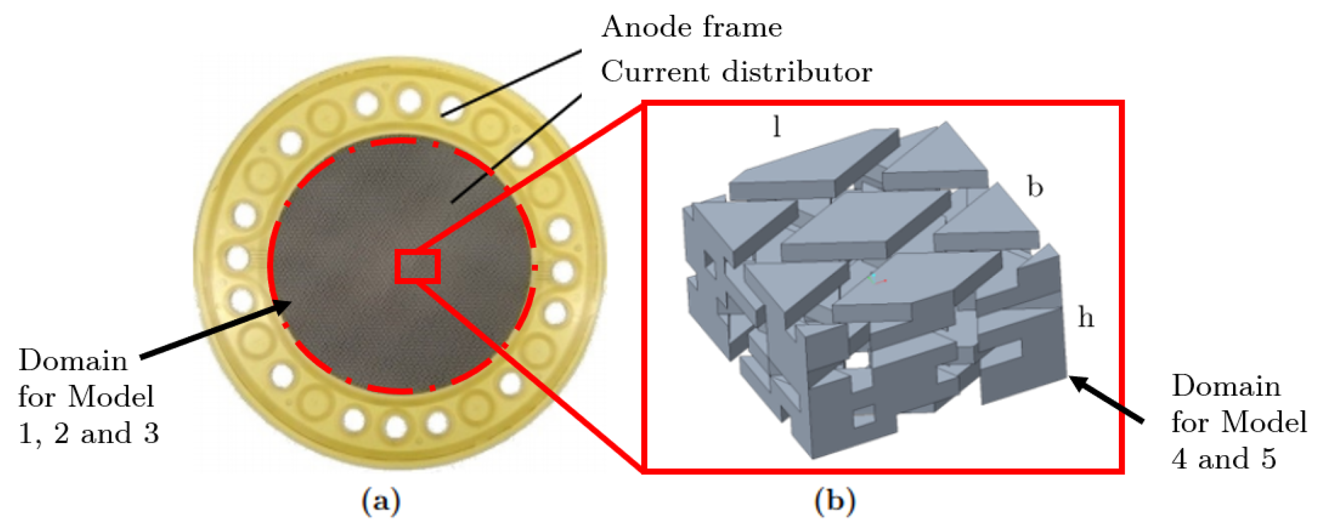
2.1. Layout of PEM Water Electrolyzer Stack

The PEM high-pressure electrolyzer stack was designed as an asymmetrical electrolyzer, meaning the system pressure of the anode and cathode side differed. The single cells were electrically connected in a bipolar configuration in filter press design and connected in series to form the cell stack. The unit had three inlet/outlet channels ((1) water inlet; (2) both water and oxygen outlet; and (3) hydrogen outlet) and two electrical connections (contact and base plate). The cell stack was placed vertically and held together by the preload between the pressure and base plate. The components of the stack are presented in Figure 2.

Asymmetrical high-pressure operation requires THE axial and radial support of the compression forces. The twelve tension rods absorb the resulting forces in axial stacking direction. In addition, the tension rods apply the preload force for a gastight sealing of the cell stack during operation. At both ends of the tension rods, nuts with washers are fitted to apply force to the stack. Synthetic washers and foils ensure that the PEM stack is electrically insulated. Disc spring columns are mounted on the upper side of the twelve tension rods with their arrangement influencing the preload force. The function of the pressure plate is to absorb forces and ensure an even contact pressure between the contacted components. Compared to a conventional, symmetrical electrolyzer stack (and fuel cell stack) the pressure plate for asymmetrical stacks was more massive due higher axial forces during operation. In addition, the pressure plate transmits the preload force to the components within the cell stack. Non-membrane electrical resistance within the cell stack is strongly dependent on the surface pressure between current-carrying components; therefore, the maximum permissible surface pressure for a given material should be targeted to minimize the contact resistance. The gold- or titanium-coated contact plate functions as the electrical connection to the positive pole of the voltage source. Sixteen pressure rings absorb the radial operating forces. The segmentation into individual pressure rings facilitates assembly and disassembly. The base plate provides the media supply and media removal. During operation, deionized water was supplied to the anode and a phase mixture of liquid water and gaseous oxygen gas was removed. The discharge of the produced and water vapour-saturated hydrogen gas also occurs via the channels in the base plate. Additionally, the base plate provides electrical contacting to the negative pole of the cell stack. The base plate and stack were securely positioned on an assembly plate. A total of 20 connected single cells, consisting of anode, cathode and membrane, form the cell stack. Lastly, two spacers were placed between the contact plate and the anode of the uppermost cell to adjust the surface pressure in the stack. The second function was for dictating the heat transfer from the uppermost anode half-cell. An even distribution of the temperature of the individual half-cells was desired to ensure the best performance and even degradation rates in each cell, since the weakest cell was limiting overall behaviour of a bipolar design [13,14].

2.2. PEM Cell Assembly

The components of a single cell are presented in Figure 3.

The anode half-cell consists of a current distributor (also called the porous transport layer (PTL)), microporous layer (MPL), seal and anode frame. Deionized water is supplied continuously and distributed evenly to the reaction site by a multi-layered current distributor. Additionally, the current distributor functions as an electrical conductor for the transfer of electrons from the reaction zone. A decisive factor in the electrolysis process is the prevention of blocking of the electrode surface by oxygen bubbles, therefore a good flow field design is of utmost importance, since it influences the spatial distribution of temperature, pressure, velocity and oxygen concentration. An additional microporous layer (MPL) is located between the distributor and the MEA to enable an even distribution of the supplied water and the removal of the oxygen gas and electrons. The MPL also dissipates the reaction heat generated at the electrode, so a high thermal conductivity is desirable. The process heat is then conducted via the current distributor to the bipolar plate and further into the water flow. The water supply and removal channels are contained on a plastic anode frame. Between the anode frame and the bipolar plate, a sealing was placed to prevent leakage.

The heart of the PEM electrolyzer is the membrane electrode assembly (MEA). A non-corrosive polymer membrane was used as the electrolyte, with catalytic layers attached to the side surfaces for the electrochemical reactions. The main task of the membrane was the conduction of hydrogen protons from the anode to the cathode side, where the ability of the membrane to absorb water influences the conductivity. The most frequently used solid state membrane in PEM fuel cells and electrolyzers is Nafion © from DuPont [15]. A further task of the diaphragm is the reduction in the permeation rates of hydrogen and oxygen due to the high-pressure difference. In asymmetric PEM electrolyzers, both significant hydrogen permeation in the direction of oxygen and oxygen permeation in the direction of hydrogen occur [16,17].

Transported hydrogen protons are reduced with electrons to form gaseous hydrogen at the cathode half-cell. The components in the cathode half-cell are analogous to those at the anode with minor differences regarding material requirements. For the material of the current distributor in the cathode, half-cell carbon paper [18] was used. For the electron supply, high electrical conductivity is required. Since there is no water recirculation to dissipate heat on the cathode path, a high thermal conductivity is required. The removal of the reaction heat is required for the lowest possible temperature gradient within the membrane and is thus decisive for degradation [19]. A hydrophobic carbon-based MPL is employed to separate the water coming from the anode side due to the electro-osmotic effect, concentration gradients and the pressure difference from the hydrogen gas. The cathode frame is identical to the anode frame and is mainly used to accommodate the MPL and current distributor as well as the outlet channels.

Lastly, the adjacent cells are electrically connected via bipolar plates, which are conducting the electrons (or current) to the adjacent half-cell, which as a result, requires the lowest possible electrical resistance. Another function of the bipolar plate is the absorption of the mechanical loads and uniform pressure distribution to the components. Finally, it provides the separation between the hydrogen and oxygen in adjacent anode–cathode half-cell pairs, therefore preventing the formation of an ignitable mixture. Mainly, gold- or titanium-plated stainless steel was used as material due to its high corrosion resistance and low contact resistances to minimize the power consumption of the stack [20].

2.3. Mathematical Model

Presented below is the mathematical model used in the CFD software.

The continuity and momentum conservation equations for the single-phase flow are described by Equations (1) and (2), respectively [12]:

$$\rho \frac{\partial p}{\partial t}+\nabla ·\left(\rho \overrightarrow{v}\right)=0$$

(1)

$$\frac{\partial }{\partial t}\left(\rho \overrightarrow{v}\right)+\nabla ·\left(\rho \overrightarrow{v}\overrightarrow{v}\right)=-\nabla p+\nabla ·\left(\stackrel{=}{\tau }\right)+\rho \overrightarrow{g}+\overrightarrow{F}$$

(2)

where $\rho$ is the density, $\overrightarrow{v}$ is the velocity vector, p is the static pressure, $\stackrel{=}{\tau }$ is the stress tensor (described below), $\rho \overrightarrow{g}$ is the gravitational body force and $\overrightarrow{F}$ is external body forces from the model-dependent source terms such as porous media. The stress tensor is given by

$$\stackrel{=}{\tau }=\mu [(\nabla \overrightarrow{v}+\nabla {\overrightarrow{v}}^t)-\frac{2}{3}\nabla ·\overrightarrow{v}I]$$

(3)

where $\mu$ is the molecular viscosity and I is the unit tensor.

For the turbulence modelling, the realizable $k-ϵ$ model solves the following transport equations for the turbulent kinetic energy k and turbulent dissipation rate $ϵ$ [12]:

$$\frac{\partial }{\partial t}\left(\rho k\right)+\frac{\partial }{\partial x_j}\left(\rho k{u}_j\right)=\frac{\partial }{\partial x_j}[(\mu +\frac{{\mu }_t}{{\sigma }_k})\frac{\partial k}{\partial x_j}]+G_k+G_b-\rho ϵ-Y_M+S_k$$

(4)

$$\frac{\partial }{\partial t}\left(\rho ϵ\right)+\frac{\partial }{\partial x_j}\left(\rho ϵu_j\right)=\frac{\partial }{\partial x_j}[(\mu +\frac{{\mu }_t}{{\sigma }_{ϵ}})\frac{\partial ϵ}{\partial x_j}]+\rho C_{1}Sϵ-\rho C_2\frac{{ϵ}^2}{k+\sqrt{\nu ϵ}}+C_{1ϵ}\frac{ϵ}{k}{C}_{3ϵ}{G}_b+S_{ϵ}$$

(5)

In these equations, $G_k$ represents the generation of turbulence kinetic energy due to the mean velocity gradients, $G_b$ is the generation of turbulence kinetic energy due to buoyancy, $Y_M$ [21] represents the contribution of the fluctuating dilatation in compressible turbulence to the overall dissipation rate, $C_2$ (= 1.9) and $C_{1ϵ}$ (= 1.44) are constants, ${\sigma }_k$ (= 1.0) and ${\sigma }_{ϵ}$ (= 1.2) are the turbulent Prandtl numbers and $S_k,S_{ϵ}$ represent additional source terms. The terms $G_k$ and $G_b$ are calculated as follows [12]:

$$G_k={\mu }_t{S}^2$$

(6)

$$G_b=\beta g_i\frac{{\mu }_t}{P{r}_t}\frac{\partial T}{\partial x_i}$$

(7)

with $S=\sqrt{2S_{ij}{S}_{ij}}$ as the modulus of the mean rate-of-strain tensor, $P{r}_t$ (= 0.85) is the turbulent Prandtl number, $g_i$ is the component of the gravitational vector in the i-th direction, $\beta =-\frac{1}{\rho }{\left(\frac{\partial \rho }{\partial T}\right)}_p$ is the coefficient of thermal expansion and ${\mu }_t=\rho C_{\mu }\frac{k^2}{ϵ}$ is the turbulent viscosity with a standard value for $C_{\mu }$ of 0.09.

$$C_1=\max [0.43,\frac{\eta }{\eta +5}];\eta =S\frac{k}{ϵ};C_{3ϵ}=\tanh |\frac{v}{u}|$$

(8)

where v is the component of the flow velocity parallel to the gravitational vector and u is the component of the flow velocity perpendicular to the gravitational vector.

Mathematical Description of the Boundary Conditions

The boundary conditions on the walls, in this case flow velocity in the direction normal to the wall surface, are presented as follows:

$$\overrightarrow{v}·\overrightarrow{n}=0$$

(9)

The boundary condition of average flow velocity normal to the surface at the inlet is presented as follows:

$$\overrightarrow{v}=-v_o\overrightarrow{n}$$

(10)

The turbulent kinetic energy and turbulent dissipation rate at the inlet are calculated according to the following equations [22]:

$$k=\frac{3}{2}{\left(v_{o}I\right)}^2$$

(11)

$$ϵ=\frac{C_{\mu }^{0.75}{k}^{1.5}}{l}$$

(12)

where I is the turbulence intensity and l is the turbulence length scale.

2.4. Simulation Model

Mesh Generations of PTL and Detail Geometry

For the various simulations presented in this paper, three different geometrical models were used for numerical calculations. Two of the models represent the whole geometrical PTL domain, whereas for the third model, only a detailed section of the geometry was considered. In the first model, the negative geometry of seven porous transport layers is meshed, as can be seen in Figure 4. The geometry shown in the figure represents only a small detailed segment of the PTL for the purpose of presentation, for the whole simulation domain of the first model, as can be seen in Figure 5a.

Due to the high complexity of the geometry and the large data size of the original CAD model, the meshing would be difficult and time consuming, therefore a simplification of the original geometry was conducted by using parallelograms to replicate the negative PTL area. The mesh was manually created using the AVL Fire © meshing tools, where the parallelograms were meshed using hexahedra. The different layers of parallelograms were connected using arbitrary connection, meaning the faces’ adjacent parallelograms did not perfectly overlap and the face fluxes will be computed using numerical interpolation [22]. A mesh sensitivity study with respect to the discretization of a single parallelogram element was performed, resulting in a maximum discretization of 5 × 5 × 4 hex elements per parallelogram and a total mesh size of approx. 2.9 million cells. The drawback of this model is that Fire © (version R2017.1) only allows single-phase flow when using arbitrary connection. To overcome the limitations of the first model regarding the number of phases in the flow and to reduce the cell count (and therefore computation time), a second geometrical model was proposed. In this model, the PTL domain is geometrically modelled (and subsequently meshed) as a single solid block, with a porosity model [22] applied in Fire ©. The increased flow resistance due to the porous structure is accounted for via an additional sink term [23] in the momentum equation. The resulting pressure drop following the Forchheimer [23] equation:

$$\frac{\partial p}{\partial x_i}=-{\alpha }_i·\mu ·u_i-{\zeta }_i·\frac{\rho }{2}·\left|u\right|·u_i$$

(13)

where $\mu$, $\rho$ and u denote the dynamic viscosity, density and velocity of the fluid, respectively. The coefficients ${\alpha }_i$ and ${\zeta }_i$ are model parameters and need to be specified by the user for the x, y and z directions. The input parameters are summarized in

Table 1. Input parameters for the porosity model.

Porosity type	Homogeneous
Porosity (=$V_H$/$V_{\mathrm{total}}$)	40%
Pressure drop model	Forchheimer
$\zeta$-values (1/m)	x = 0, y = 0, z = 0
$\alpha$-values (1/m2)	x = 1010, y = 1010, z = 104

.

The porosity percentage was derived from the CAD model, whereas the $\alpha$- and $\zeta$- values were determined by data fitting the pressure loss between the inlet and outlet of the porosity model to the pressure loss obtained through measurements. With the $\zeta$- values set to 0, the Equation (13) is simplified to Darcy’s law:

$$\frac{\partial p}{\partial x_i}=-{\alpha }_i·\mu ·u_i$$

(14)

The two approaches are summarized in

Table 2. Summary of the geometrical models.

	Model 1	Model 2
Description	Basic model	Porosity model
Simulation	Single phase	Single and multiphase
Structure	7 layers, structured	Unstructured
Connection	Arbitrary	-
Element	Parallelogram	-
Element discretization	5 × 5 × 4	-
Cell type	Hexahedron	Polyhedron
Mesh size (cells)	2,917,888	222,425

.

For the more detailed flow analysis within the complicated geometry, a very fine discretization is required. Meshing the whole domain with such fine cells was not feasible due to limited computing resources, therefore only a small detailed section of the current distributor (see Figure 5) will be calculated. In addition to AVL Fire ©, ANSYS Fluent © was used for the simulation. The simulations were carried out on a Linux server with two Intel © Xeon © E5-2687W CPUs for a total of 24 logical cores and 128 GB RAM. For the model generation, a section of the current distributor with the dimensions (l × w × h) of 3 × 3 × 1.7 mm was chosen. The CAD derivation of the detailed section corresponds to the negative form of the current distribution frame which also defines the flow area. The mesh was constructed using the automatic meshing tools and exclusively consists of tetrahedra with a total of approximately three million cells. An overview of the simulation models and their goals is summarized in

Table 3. Overview of the simulation models presented in this work and their goals.

Nr	Domain	Geometry	Phases	Goal
Model 1	Whole PTL	Exact geometry	Single	Investigation of temperature, pressure and velocity distributions inside the PTL
Model 2	Whole PTL	Porosity model	Single	Reproduction of results from Model 1 with significant reduction in computation time
Model 3	Whole PTL	Porosity model	Two-phase Eulerian	Expansion of Model 2 to include the gas phase to investigate gas bubble distribution inside the PTL
Model 4	Detailed section of the PTL	Exact geometry of the section	Two-phase Eulerian	Detailed investigation of local phenomena regarding gas bubble entrapment using the Eulerian approach
Model 5	Detailed section of the PTL	Exact geometry of the section	Two-phase VOF	Detailed investigation of local phenomena regarding gas bubble entrapment using the VOF approach

.

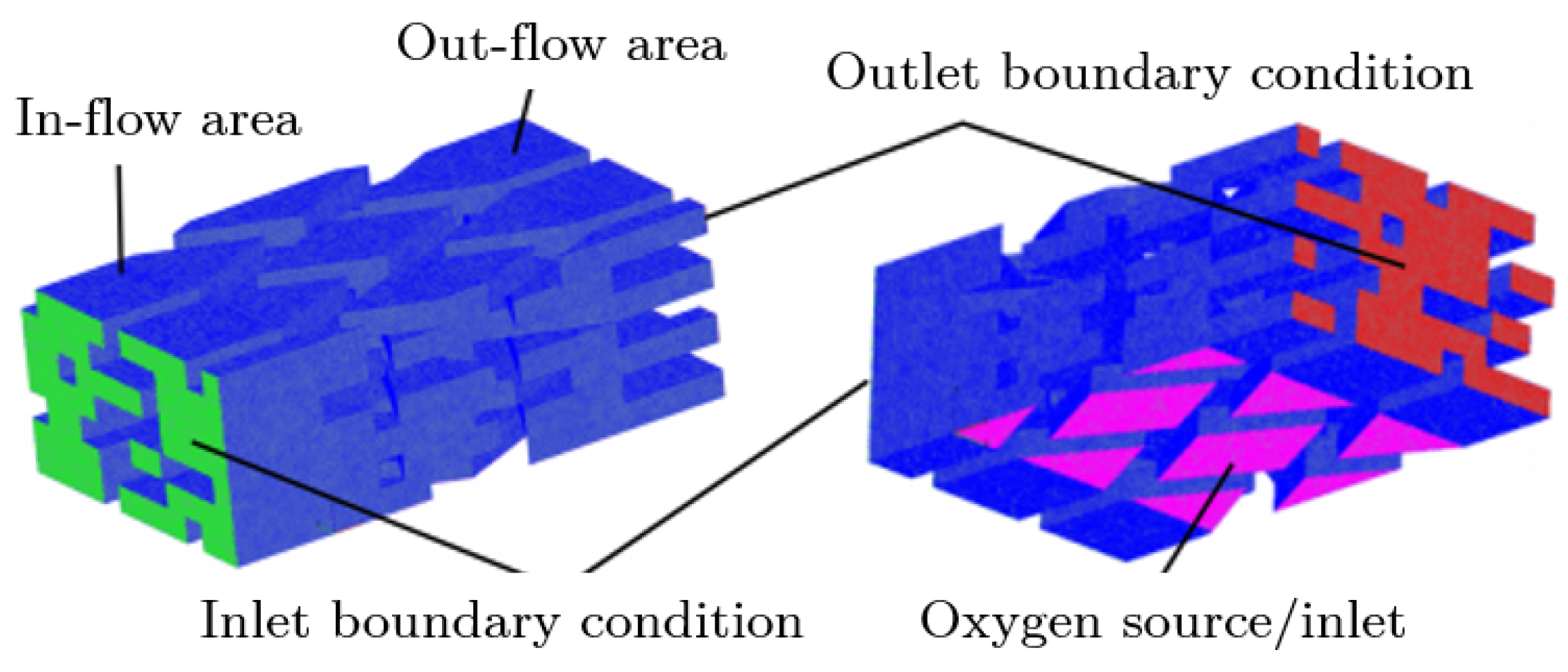
2.5. Initial and Boundary Conditions

The boundary conditions (BCs) for both models include the inlet, outlet and wall. Additionally, the second model has an extra boundary condition at the PTL face bordering the anode as the oxygen source for the multiphase case. Due to software limitations, it was not possible to simultaneously define a mass source (in this case oxygen) and sink (water) at the same boundary face. Since the water amount supplied by the pump is over a factor of 200 higher than the amount that is consumed for the chemical reaction (stoichiometric ratio >200) and the water amount transported through the membrane was much smaller compared to the total flow (experimental data have shown that 1/30 of the total flow was transported through the membrane) the water consumption due to the chemical reaction and the water transport due to diffusion, electro-osmosis and pressure gradient will not be considered in this simulation. Neglecting the water flux means that the net (phase-averaged) velocity points in the wrong direction (to the inside of the PTL) at the oxygen source boundary. However, given the high water stoichiometry, the contribution of oxygen to the net outlet flow is small in comparison and the composition dependence of density is much more important for the fluid dynamics. Therefore, only the oxygen source is defined at the boundary face for the multiphase case. Subsequently, follows a description of the BCs.

2.5.1. Inlet Boundary Condition

The following physical quantities are required for the inlet boundary condition:

• Velocity (u, v, w);
• Temperature T;
• Turbulent properties (turbulent kinetic energy k, length scale L, dissipation $\epsilon$);
• Volume fraction $\phi$ (for the multiphase case).

The velocity is specified normal to the inlet face and is determined from the volume flow of the recirculation pump. A total volume flow of 5.4 L/min is being fed by the pump of a 20-cell stack. Under the assumption of an equal distribution of the water feed to each of the cells and an inlet channel cross-sectional area of 2 mm², the resulting velocity is 2.25 m/s. A typical operational temperature of 80 °C is given at the inlet. Furthermore, it was seen from experimental data that the maximum temperature difference between the inlet and outlet is in the range of 7 °C and the effect on the flow field is minimal, therefore a constant temperature of 80 °C is applied to the whole simulation domain. Some further assumptions must be made to define the turbulent properties at the inlet. The k-$\epsilon$ turbulence model was used, as it is suitable for preliminary flow field calculations with physical phenomena such as multi-phase interactions [24,25]. For the turbulent intensity (ration between velocity fluctuation $u^{\prime }$ due to turbulence and the average velocity $U_{\infty }$ [12]) a typical value of 10% is found in the literature [22,26]. For the turbulent length scale, a value of 10% of the hydraulic diameter was proposed in the literature [26]. Following these assumptions, the turb. kinetic energy k and turb. diss. rate $\epsilon$ are calculated by Fire © using the Kolmogorov formulation [22]. A volume fraction of 100% water is specified for the multiphase case.

Table 4. Inlet Boundary Condition.

Quantity	Value	Unit
Velocity (normal to inlet face)	2.25	m/s
Volume fraction of water	100	%
Temperature	80	°C
Turbulence intensity	10	%
Turbulence length scale in % of $d_h$	10	%
Turbulent kinetic energy	0.029	m2/s2
Turbulence length scale	0.071	mm
Turbulent dissipation rate	11.2	m2/s3

summarizes the boundary conditions at the inlet.

2.5.2. Outlet Boundary Condition

For simplicity, a static pressure of 1.013 bar was applied at the outlet.

2.5.3. Wall Boundary Condition

A constant temperature of 80 °C and a wall roughness of 0.5 (default value) were applied at the wall BC.

2.5.4. Oxygen Source Boundary Condition

The amount of produced oxygen was determined from Faraday’s law [27]:

$${\dot{n}}_{{\mathrm{O}}_2,\mathrm{prod}}=\frac{I}{z·F}$$

(15)

where ${\dot{n}}_{{\mathrm{O}}_2,\mathrm{prod}}$ is the molar flux, I is the electrical current at which the cell is operated, z is the number of transferred electrons and F is Faraday’s constant. For the simulations a fixed operating point at 160 A electrical current was set, whereas z = 4 for the PEM electrolysis reaction, resulting in 0.025 mol/min O₂. The normal velocity and the turbulent quantities were determined to be analogous to the procedure described for the inlet BC and are summarized in

Table 5. Oxygen source boundary condition.

Quantity	Value	Unit
Molar flux O2	0.025	mol/min
Mass flux O2	13.3	mg/s
Volume flux O2	$1.22·{10}^{-5}$	m3/s
Surface area of the BC face	5.67	cm2
Velocity (normal to inlet face)	$2.145·{10}^{-3}$	m/s
Volume fraction of oxygen	100	%
Temperature	80	°C
Turbulence intensity	5	%
Turbulence length scale in % of $d_h$	5	%
Turbulent kinetic energy	1.727 $·{10}^{-8}$	m2/s2
Turbulence length scale	0.069	mm
Turbulent dissipation rate	5.33 $·{10}^{-9}$	m2/s3

.

2.5.5. Boundary Conditions for Detailed Section

The boundary conditions for the detailed section are seen in Figure 6. The inlet velocity was based on the simulation results from the first two models and was estimated at 0.05 m/s. The turbulent properties were determined as analogous to the previous models. Since no data for the pressure at the outlet were available, a static pressure of 1.013 bar was assumed, similarly to the previous models. The area of the oxygen source BC and the specified velocity differed for the Eulerian multiphase and the volume-of-fluid model. The BC for the Eulerian model is as seen in Figure 6 with a constant velocity $v_{{\mathrm{O}}_2,\max }=2.145·{10}^{-3}$ m/s. For the VOF model, a dynamic velocity with a frequency of 4 Hz was defined to simulate the oxygen bubble detachment according to the following formula:

$$v_{{\mathrm{O}}_2}\left(t\right)=\frac{v_{{\mathrm{O}}_2,\max }}{2}+\frac{v_{{\mathrm{O}}_2,\max }}{2}·\cos \left(\omega t\right)$$

(16)

The area for the oxygen source was modified as presented in Figure 7. Instead of the whole face as with the Eulerian model, only circular patches on the bottom face near the inlet are defined as the oxygen source. The settings are summarized in

Table 6. Boundary conditions for the detailed section.

Quantity	Inlet	Oxygen Source	Unit
Velocity (normal to inlet face)	0.05	$2.145·{10}^{-3}$	m/s
Volume fraction	100% water	100% oxygen	%
Temperature	80	80	°C
Turb. length scale in % of d_h	10	5	%
Turb. kin. energy	0.085	0.085	m2/s2
Turb. length scale	0.089	0.067	mm
Turb. dissipation rate	9.33	2.33	m2/s3

.

2.6. Multiphase Numerical Models

Different mathematical models can be used for multiphase flows, with different approaches for the mass, momentum and enthalpy interfaces [28]. Due to low solubility of oxygen in water at the operating conditions of 3 bar and 80 °C [29], the phases were considered immiscible. Additionally, no phase change occurred in either of the two phases. Therefore, no interfacial mass exchange will be considered. For the momentum exchange, an additional term is present in the momentum equation, taking into account the forces between phases due to the surface tension. Since a constant temperature of 80 °C was assumed in the whole simulation domain, and therefore no temperature gradients for the enthalpy exchange are present, no enthalpy exchange is considered. A quick overview of typical multiphase models found in CFD software is presented below.

2.6.1. Mixture Model

The mixture model [12] is a simplified multiphase model, where one set of mass, momentum and energy equations is solved for the fluid mixture. This model allows the phases to be interpenetrating and as such, any value between 0 and 1 is possible for the volume fraction ${\phi }_i$ in a control volume. The mixture properties such as density and viscosity are calculated as follows:

$${\rho }_{\mathrm{mix}}=\sum _i{\phi }_i·{\rho }_i,{\mu }_{\mathrm{mix}}=\sum _i{\phi }_i·{\mu }_i$$

(17)

The mass-averaged velocity of the mixture is calculated as follows:

$${\overrightarrow{v}}_{\mathrm{mix}}=\frac{{\displaystyle \sum _i}{\phi }_i{\rho }_i{\overrightarrow{v}}_i}{{\rho }_{\mathrm{mix}}}$$

(18)

The fluid properties and velocities in Equations (1) and (2) are replaced by the mixture properties and the velocity of the mixture. An additional term for the drift velocity of the i-th secondary phase ${\overrightarrow{v}}_{dr,i}={\overrightarrow{v}}_i-{\overrightarrow{v}}_{\mathrm{mix}}$ is added to the right side of the momentum equation: $-\nabla ·({\displaystyle \sum _i}{\phi }_i{\rho }_i{\overrightarrow{v}}_{dr,i}{\overrightarrow{v}}_{dr,i})$.

The fluid properties for water and oxygen at 80 °C and 1 bar were extracted from the NIST database [29]. Since the temperature remained constant and the change in density and viscosity was negligible in the pressure range between 1 and 3 bar, the properties were kept constant for all simulation cases. The fluid properties of water and oxygen are summarized in

Table 7. Fluid properties.

Fluid	Density (kg/m3)	Viscosity (kg/m·s)
Water	971.79	35.435$·{10}^{-5}$
Oxygen	1.0900	2.3395$·{10}^{-5}$

.

2.6.2. Volume-of-Fluid

The volume-of-fluid method (VOF) [12] is used for calculating the phase interfaces between immiscible fluids. The volume fractions were calculated for each cell according to the equation below:

$$\frac{\partial \phi }{\partial t}+\nabla ·\left(\phi \overrightarrow{v}\right)=0$$

(19)

where $\overrightarrow{v}$ is the velocity vector. Three states can occur in respect to the value of $\phi$:

• $\phi$ = 0, no continuous phase in the cell;
• $\phi$ = 1, only continuous phase in the cell;
• 0 < $\phi$ < 1, phase boundary interface.

One set of mass, momentum and energy equations was solved analogous to the mixture model. An additional term accounting for the surface tension between phases is present in the momentum equation. In this work, the gas–liquid interface was transiently tracked until t = 1 s.

2.6.3. Eulerian Model

The Eulerian multiphase model [12,28] can account for dispersed–continuous (i.e., gas bubble dissolved in a fluid) and continuous–continuous (immiscible fluids) phase interfaces. A set of governing equations (mass, momentum, enthalpy) is solved for each of the phases separately and accounts for interfacial mass, momentum and enthalpy transport between the phases. An additional transport equation is solved for the volume fraction of each additional phase. The phases share a common pressure field.

3. Results and Discussion

In this section, the results of the single-phase flow (water) followed by the results of the two-phase flow (water–oxygen) will be presented and discussed. The main points of interest are the pressure and velocity distributions of the flow field. Additionally, the volume fraction distribution and phase interface are of interest for the two-phase flow. Gravitational forces and buoyancy are considered for all presented cases. The letters I and O in all of the presented plots denote the inlet and outlet, respectively.

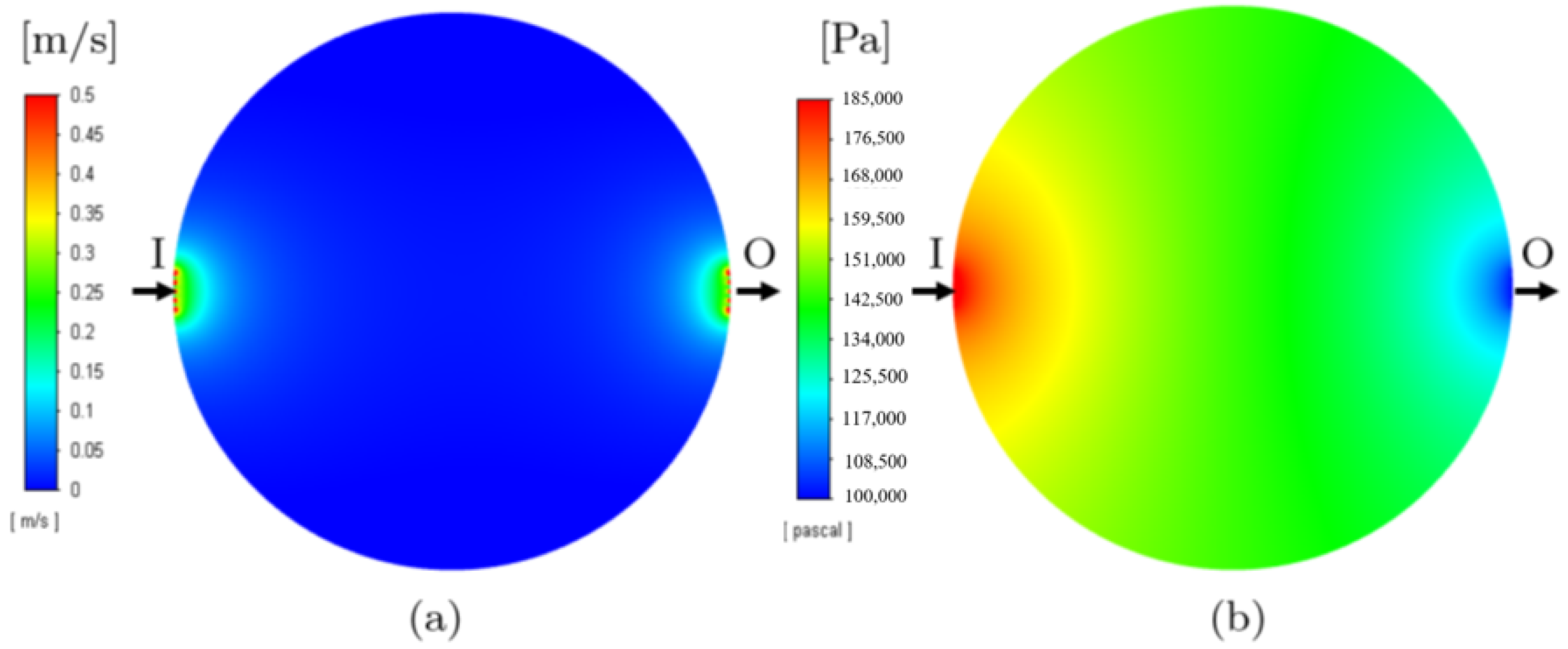
3.1. Single-Phase Models

Figure 8 shows the surface plots of velocity and pressure distribution from a top–down view of the exact geometry model. Water enters the domain through flow channels from the inlet (I) and flows via the current distributor to the outlet (O). The complex geometrical structure of the current distributor evenly distributes the incoming water over the entire electrode surface, as can be seen by the uniform velocity flow field in Figure 8a. It can also be seen that the highest velocities are found at the inlet and outlet channels and at the transition of the channels into the transport layer. The velocity magnitude distribution in the transport layers is influenced by its geometrical shape. The velocity magnitude decreases with increasing cross-sectional area in accordance with the continuity equation, assuming the density is constant. The assumption of a constant density is valid for this simulation, since the flow is incompressible [30] and the temperature was assumed to be uniform and constant through the whole simulation domain. Therefore, a decrease in velocity occurs from the entrance to the centre of the geometry. In contrast, the reduction in the area from the centre to the output leads to acceleration. The area with the highest velocity also corresponds to the area where the biggest pressure loss occurs, as can be seen from Figure 8b. Furthermore, the pressure over the transport layer area is almost constant, with an almost negligible pressure loss. A total calculated pressure loss of 0.83 bar is in good agreement with obtained experimental data, where the measured pressure loss was between 0.80 and 0.85 bar.

The results of the porous volume model are presented in Figure 9, again depicting the velocity and pressure distributions in the flow field. The surface plots show good agreement to the exact geometry model regarding absolute values of velocity and pressure as well as flow field distribution. By selecting the proper porosity parameters (see Table 1), the pressure and velocity distributions can be adequately modelled using a simplified geometry. The main advantage of the simplified geometry approach is a significant reduction in simulation time and computing resources.

3.2. Two-Phase Models

For the water–oxygen flow, the Eulerian multiphase approach was used in Ansys Fluent ©. The distributions of velocity, pressure and oxygen volume fraction of the porous volume model are depicted in Figure 10. A comparison with the results of the single-phase flow (Figure 9) supports the correct tendencies of the two-phase model simulation results. Due to the oxygen input, higher velocities prevail in the entire flow area, in turn resulting in a higher pressure loss. The simulated pressure loss of 1.7 bar is in good agreement with the measured pressure loss of 1.6–1.7 bar. The distribution of the oxygen volume fraction is also plausible, with a visible increase from inlet to outlet (see Figure 10c). It can be seen that oxygen tends to mostly accumulate at the outer wall on the outlet half of the circular PTL, with the oxygen volume fraction reaching above 85%. No phase boundary interface between water and oxygen is calculated, rather the calculated volume fractions correspond to a statistical distribution of the volume fractions of both phases in the flow area.

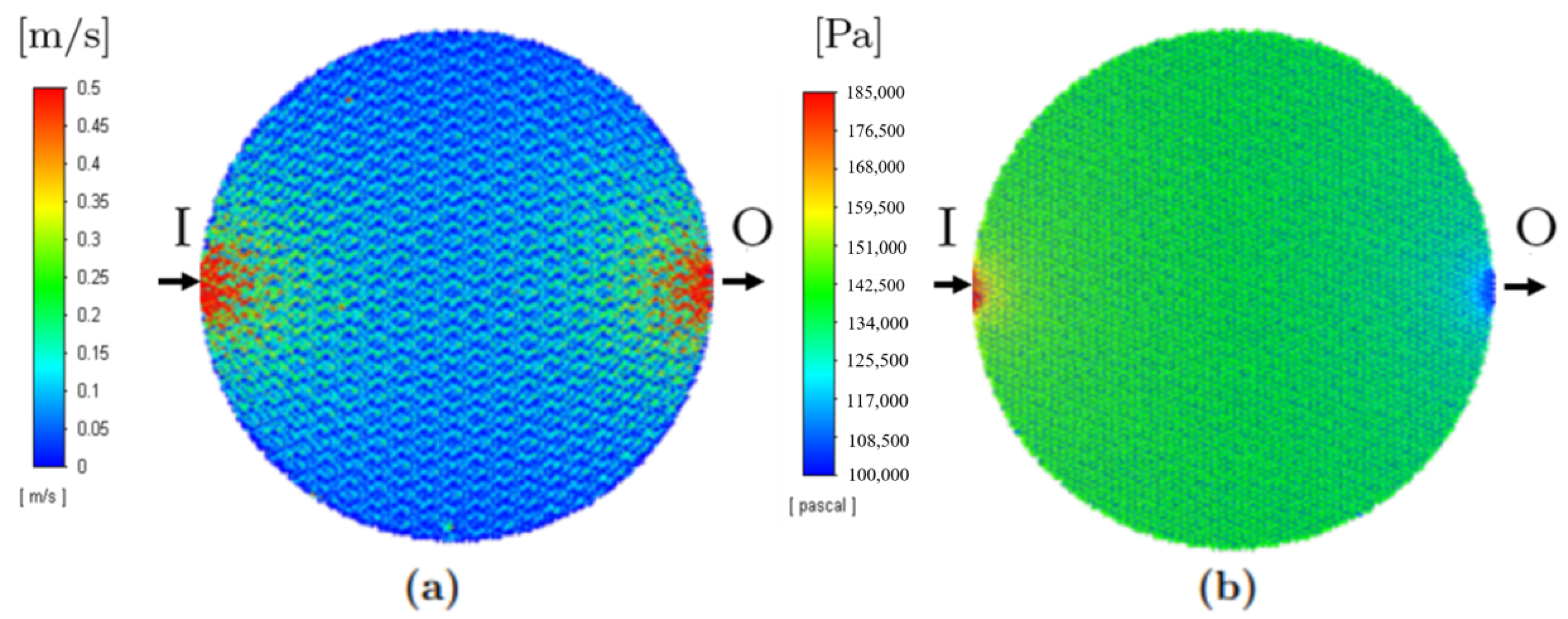
3.3. Detailed Geometry

The simulation results in the following sections refer to representations in the section planes 1, 2 and 3 according to Figure 11. Section plane 2 is in the centre and planes 1 and 3 have an edge distance of 0.5 mm each. I denotes the inlet and O the outlet. Results for the Eulerian and the VOF model will be presented.

The Eulerian multiphase model calculates a separate velocity field for each phase. Figure 12 shows the velocity fields of water (a) and oxygen (b) in the three section planes. A difference in the velocity fields is mainly in areas with low oxygen content, such as in the whole inlet area (I) of Figure 12b, where the velocity is 0. The velocity distribution in the detailed section is by no means uniform. Especially at narrow places, the velocity magnitude reaches three times the 0.05 m/s prescribed at the inlet. The distribution of oxygen volume fraction in the three defined planes is pictured in Figure 13. In the simulation, oxygen and water phases are represented by a continuous area. Furthermore, it can be seen that the water flow leads to a transport of the oxygen introduced at the bottom side towards the outlet (O). It can be seen in planes 2 and 3 that the oxygen reaches the uppermost layers of the PTL near the outlet due to buoyancy. At the lower edge of the image in plane (1), areas can be seen in which vortex formation and the backflow of oxygen occurs, resulting in oxygen entrapment. Such areas should be avoided when constructing new PTL geometries.

In contrast to the Eulerian model, a single velocity field is calculated for the VOF model. The phase interface between water and oxygen is simulated transiently for a simulation time of 1 s. For the presentation of the results, the position of the planes is slightly adjusted to be positioned exactly in the centre of the circular shapes of the oxygen boundary surface (see Figure 14). The velocity distribution (a) and the oxygen volume fraction (b) are shown in Figure 14. The simulated velocity distribution by the VOF method shows local areas with high velocities near the oxygen source, as shown in Figure 14a. In plane (1) in Figure 14b again the backflow of oxygen upstream in the direction of the inlet is visible. This is due to the geometrical design of the current distributor by expanded metal layers. The formed oxygen cannot reach the outlet via the shortest way, but has to be transported upstream or in the vertical direction first due to the geometry. From Figure 14b, it can also be seen that no phase interface between water and oxygen is visible. The two phases are rather represented as a mixed phase in almost the entire area, which goes against our assumption of oxygen insolubility in water. The reason for this is the insufficient spatial discretization of the flow region. The three million cell count is too low to sufficiently capture the bubble flow. However, due to the limited computer capacity and simulation time, the number of cells cannot be increased arbitrarily.

4. Conclusions

Five models with different levels of detail and different goals were developed and investigated in this work. The first model attempted to capture the whole PTL domain with an as-exact-as-possible geometry. Single-phase flow simulations using the first model showed good agreement with measurements and can be used for an evaluation of the uniform distribution of the water flow field in the anode half-cell. A uniform distribution is of crucial importance for efficiency and durability. The multi-layered PTL in the anode half-cell of the analysed high-pressure PEM electrolyzer fulfils this task well and evenly distributes the water flowing into the cell over the electrode. A validation of the simulation results of the single-phase flow was carried out by measuring the pressure loss of the pure water flow. Due to the long simulation times of the first model, a second model was developed using the porous volume approach for the PTL geometry. The simplified model could replicate the results of the first model with a significant reduction in simulation time. To understand the oxygen distribution inside the flow field, the second model was expanded to include the gas phase. The results of multiphase calculations for the third model with porous volume approach are plausible and show reasonable tendencies in the distributions of velocity, pressure and volume fractions of the phases, however, these cannot capture local phenomena such as bubble entrapment. For detailed observations of flow phenomena, a very fine spatial discretization must be chosen, resulting in high mesh cell counts and therefore requiring great computing power. Due to these limitations, only a small section of the PTL was modelled for the detailed flow investigations. For the two-phase flow, two approaches were used: Eulerian model (model 4) and VOF model (model 5). The Eulerian model showed especially promising results, where areas with backflow could clearly be seen, whereas for the VOF model, an even finer mesh would be needed to produce a clearer phase boundary, prolonging the simulation time. In conclusion, it can be said that 3D-CFD is suitable as an auxiliary development tool for PEM electrolysis, but further development of the commercially available CFD models is required. For the simulation of the numerically complex two-phase flows, further development is especially necessary to facilitate the use of conventional computers for the simulations, circumventing the necessity of supercomputers or computer clusters. Subsequently, simulations based on the model with porous a volume approach can be performed. For this purpose the parameters of the porosity model were first validated by experimental measurements. In addition, the simulation model can be adapted to include the entire cell stack, taking into account the heat transfer phenomena between the components.

References

1. Klell, M.; Eichlseder, H.; Trattner, A. Wasserstoff in der Fahrzeugtechnik. Erzeugung, Speicherung, Anwendung, 4th ed.; Springer: Berlin, Germany, 2017. [Google Scholar]
2. Nie, J.; Chen, Y. Numerical modeling of three-dimensional two-phase gas–liquid flow in the flow field plate of a PEM electrolysis cell. Int. J. Hydrogen Energy 2010, 35, 3183–3197. [Google Scholar] [CrossRef]
3. Hoeh, M.A.; Arlt, T.; Kardjilov, N.; Manke, I.; Banhart, J.; Fritz, D.L.; Ehlert, J.; Lüke, W.; Lehnert, W. In-Operando Neutron Radiography Studies of Polymer Electrolyte Membrane Water Electrolyzers. ECS Trans. 2015, 69, 1135–1140. [Google Scholar] [CrossRef]
4. Arbabi, F.; Montazeri, H.; Abouatallah, R.; Wang, R.; Bazylak, A. Three-Dimensional Computational Fluid Dynamics Modelling of Oxygen Bubble Transport in Polymer Electrolyte Membrane Electrolyzer Porous Transport Layers. J. Electrochem. Soc. 2016, 163, F3062–F3069. [Google Scholar] [CrossRef]
5. Carmo, M.; Fritz, D.L.; Mergel, J.; Stolten, D. A comprehensive review on PEM water electrolysis. Int. J. Hydrogen Energy 2013, 38, 4901–4934. [Google Scholar] [CrossRef]
6. Arbabi, F. Oxygen Bubble Propagation in Polymer Electrolyte Membrane Electrolyzer Porous Transport Layers. Ph.D. Thesis, University of Toronto, Toronto, ON, USA, 2017. [Google Scholar]
7. Nie, J.; Chen, Y.; Cohen, S.; Carter, B.D.; Boehm, R.F. Numerical and experimental study of three-dimensional fluid flow in the bipolar plate of a PEM electrolysis cell. Int. J. Therm. Sci. 2009, 48, 1914–1922. [Google Scholar] [CrossRef]
8. Olesen, A.C.; Rømer, C.; Kær, S.K. A numerical study of the gas-liquid, two-phase flow maldistribution in the anode of a high pressure PEM water electrolysis cell. Int. J. Hydrogen Energy 2016, 41, 52–68. [Google Scholar] [CrossRef] [Green Version]
9. Han, B.; Mo, J.; Kang, Z.; Yang, G.; Barnhill, W.; Zhang, F.Y. Modeling of two-phase transport in proton exchange membrane electrolyzer cells for hydrogen energy. Int. J. Hydrogen Energy 2017, 42, 4478–4489. [Google Scholar] [CrossRef] [Green Version]
10. Aubras, F.; Deseure, J.; Kadjo, J.J.; Dedigama, I.; Majasan, J.; Grondin-Perez, B.; Chabriat, J.P.; Brett, D.J.L. Two-dimensional model of low-pressure PEM electrolyser: Two-phase flow regime, electrochemical modelling and experimental validation. Int. J. Hydrogen Energy 2017, 42, 26203–26216. [Google Scholar] [CrossRef]
11. Zinser, A.; Papakonstantinou, G.; Sundmacher, K. Analysis of mass transport processes in the anodic porous transport layer in PEM water electrolysers. Int. J. Hydrogen Energy 2019, 42, 28077–28087. [Google Scholar] [CrossRef]
12. ANSYS, Inc. Ansys Fluent Theory Guide; 2020R1; ANSYS, Inc.: Canonsburg, PA, USA, 2020. [Google Scholar]
13. Bessarabov, D.; Wang, H.; Li, H.; Zhao, N. PEM Electrolysis for Hydrogen Production: Principles and Applications; Taylor-Francis Group: Boca Raton, FL, USA, 2016. [Google Scholar]
14. Haas, C. Entwicklung Eines 3D-CFD Simulationsmodells Eines PEM-Elektrolysemoduls. Master’s Thesis, Technische Universität Graz, Institut für Verbrennungskraftmaschinen und Thermodynamik, Graz, Austria, 2018. [Google Scholar]
15. Rangel-Cardenas, A.L.; Koper, G.J.M. Transport in Proton Exchange Membranes for Fuel Cell Applications—A Systematic Non-Equilibrium Approach. Materials 2017, 10, 576. [Google Scholar] [CrossRef] [PubMed] [Green Version]
16. Fellinger, T. Entwicklung Eines Simulationsmodells für Eine PEM-Hochdruckelektrolyse. Master’s Thesis, Technische Universität Graz, Institut für Verbrennungskraftmaschinen und Thermodynamik, Graz, Austria, 2016. [Google Scholar]
17. Sartory, M.; Wallnöfer-Ogris, E.; Salman, P.; Fellinger, T.; Justl, M.; Trattner, A.; Klell, M. Theoretical and experimental analysis of an asymmetric high pressure PEM water electrolyser up to 155 bar. Int. J. Hydrogen Energy 2017. [Google Scholar] [CrossRef]
18. Toray Industries, Inc. Available online: http://www.toray.com (accessed on 11 May 2018).
19. Moseley, P.-T.; Garche, J. Electrochemical Energy Storage for Renewable Sources and Grid Balancing; Elsevier: Amsterdam, The Netherlands, 2014. [Google Scholar]
20. Bargel, H.-J.; Schulze, G. Werkstoffkunde; Springer: Berlin/Heidelberg, Germany; New York, NY, USA, 2013. [Google Scholar]
21. Sarkar, S.; Balakrishnan, L. Application of a Reynolds-Stress Turbulence Model to the Compressible Shear Layer; Final Report; Institute for Computer Applications in Science and Engineering: Hampton, VA, USA, 1990. [Google Scholar]
22. AVL List GmbH. Fire R2017.1 Documentation; Documentation AVL FIRE Version R2017.1; AVL List GmbH: Graz, Austria, 2018. [Google Scholar]
23. AVL List GmbH. Porosity; Documentation AVL FIRE Version R2017.1; AVL List GmbH: Graz, Austria, 2018. [Google Scholar]
24. AVL List GmbH. Fire CFD Solver User Manual; Documentation AVL FIRE Version R2020.1; AVL List GmbH: Graz, Austria, 2020. [Google Scholar]
25. Argyropoulos, C.D.; Markatos, N.C. Recent advances on the numerical modelling of turbulent flows. Appl. Math. Model. 2015, 39, 693–732. [Google Scholar] [CrossRef]
26. Tu, J.; Yeoh, G.-H.; Liu, C. Computational Fluid Dynamics—A Practical Approach, 2nd ed.; Butterworth-Heinemann: Oxford, UK, 2012. [Google Scholar]
27. Atkins, P.-W.; de Paula, J. Physikalische Chemie, 5th ed.; Wiley: Weinheim, Germany, 2013. [Google Scholar]
28. AVL List GmbH. Eulerian Multiphase; Documentation AVL FIRE Version R2017.1; AVL List GmbH: Graz, Austria, 2018. [Google Scholar]
29. NIST Chemistry Webbook. Available online: http://webbook.nist.gov/chemistry/ (accessed on 1 March 2018).
30. Ferziger, J.-H.; Peric, M. Numerische Strömungsmechanik, 2nd ed.; Springer: Berlin/Heidelberg, Germany; New York, NY, USA, 2002. [Google Scholar]
Figure 1. Proton-exchange membrane (PEM) cell consisting of the bipolar plates (BPPs), the porous transport layers (PTLs) on the anode and cathode side and the membrane electrode assembly (MEA), consisting of an anode (A), membrane (M) and cathode (C) [3].
Processes 09 00968 g001
Figure 2. PEM stack.
Processes 09 00968 g002
Figure 3. PEM cell assembly.
Processes 09 00968 g003
Figure 4. Negative form of a small segment of the PTL for Model 1.
Processes 09 00968 g004
Figure 5. Simulation domains of the different models, where (a) represents the whole PTL domain used for models 1–3 and (b) represents a small section of the PTL used for models 4 and 5.
Processes 09 00968 g005
Figure 6. Boundary condition for the detailed Eulerian model.
Processes 09 00968 g006
Figure 7. Boundary condition for the detailed volume-of-fluid model.
Processes 09 00968 g007
Figure 8. Distribution of (a) velocity and (b) pressure of the detailed geometry model.
Processes 09 00968 g008
Figure 9. Distribution of (a) velocity and (b) pressure of the porous volume model.
Processes 09 00968 g009
Figure 10. Distribution of (a) velocity; (b) pressure; and (c) oxygen volume fraction of the porous volume model.
Processes 09 00968 g010
Figure 11. Cutting planes.
Processes 09 00968 g011
Figure 12. Distribution of (a) velocity of H 2 O and (b) velocity of O 2 of the Eulerian multiphase model.
Processes 09 00968 g012
Figure 13. Oxygen volume fraction of the Eulerian multiphase model.
Processes 09 00968 g013
Figure 14. Distribution of (a) velocity of mixture and (b) volume fraction of O 2 of the volume-of-fluid model.
Processes 09 00968 g014