Article

Particle Lagrangian CFD Simulation and Experimental Characterization of the Rounding of Polymer Particles in a Downer Reactor with Direct Heating

by
Juan S. Gómez Bonilla
1,2,3,
Laura Unger
1,2,
Jochen Schmidt
1,2,3,
Wolfgang Peukert
1,2,3 and
Andreas Bück
1,2,3,*
1
Institute of Particle Technology, Friedrich-Alexander-Universität Erlangen-Nürnberg, Cauerstraße 4, D-91058 Erlangen, Germany
2
Interdisciplinary Center for Functional Particle Systems, Friedrich-Alexander-Universität Erlangen-Nürnberg, Haberstraße 9a, D-91058 Erlangen, Germany
3
Collaborative Research Center 814—Additive Manufacturing, Am Weichselgarten 9, D-91058 Erlangen, Germany
*
Author to whom correspondence should be addressed.
Processes 2021, 9(6), 916; https://doi.org/10.3390/pr9060916
Submission received: 26 April 2021 / Revised: 14 May 2021 / Accepted: 17 May 2021 / Published: 23 May 2021

Abstract

:
Polypropylene (PP) powders are rounded at different conditions in a downer reactor with direct heating. The particles are fed through a single central tube, while the preheated sheath gas is fed coaxially surrounding the central aerosol jet. The influence of the process parameters on the quality of the powder product in terms of particle shape and size is analyzed by correlating the experimental results with the flow pattern, residence time distribution of the particles and temperature distribution predicted by computational fluid dynamics (CFD) simulations. An Eulerian–Lagrangian numerical approach is used to capture the effect of the particle size distribution on the particle dynamics and the degree of rounding. The simulation results reveal that inlet effects lead to inhomogeneous particle radial distributions along the total length of the downer. The configuration of particle/gas injection also leads to fast dispersion of the particles in direction of the wall and to particle segregation by size. Broad particle residence time distributions are obtained due to broad particle size distribution of the powders and the particles dispersion towards the wall. Lower mass flow ratios of aerosol to sheath gas are useful to reduce the particle dispersion and produce more homogenous residence time distributions. The particles’ residence time at temperatures above the polymer’s melting onset is determined from the simulations. This time accounts for the effective treatment (rounding) time of the particles. Clear correlations are observed between the numerically determined effective rounding time distributions and the progress of shape modification on the particles determined experimentally.

1. Introduction

Particle shape plays an important role in many processes in the chemical, pharmaceutical and cosmetic industries. Powder products require a specific particle morphology depending on their application: polygonal angular hard particles are required for the production of abrasive materials [1], flat plate-like particles increasing light reflection are used as pigments for cosmetics, inks and coatings [2], while spherical particles are preferred in applications, where free-flowing powders are required, e.g., for toner or in 3D printing [3,4,5,6]. Therefore, the development of processes to control particle morphology has become increasingly important in particle technology.
One process of particle morphology modification is the rounding of irregular-shaped particles (also called spheronization). This process has been employed for the production of spherical particles of metals [7,8,9,10,11], ceramics [12], polymers [5,6,13,14,15,16,17] and pharmaceutical products [18]. Depending on the mechanical and thermal properties of the particles, rounding can be achieved by mechanical and thermal approaches. Mechanical approaches use the effect of particle abrasion and deformation upon impact to achieve spherical particles using e.g., dry impact comminution devices [7,18,19,20]. Thermal approaches involve the melting of particles dispersed in a fluid and the consequent rounding of the produced droplets driven by their surface tension. Solid spherical particles are then produced by cooling. Depending on the thermal properties of the material to be rounded different heat sources and levels of heat are required. Rounding of particles has been achieved using thermal plasmas [8,9] and plasma rotating electrodes [10,11], flames [12] and pulsed electron beam irradiation [21], using different reactor configurations.
Due to the relatively low melting temperatures of polymers compared to other materials, the rounding of polymer powders has been mainly investigated using heated downer reactors [5,6,15,16,17]. Downer reactors (in their fully developed flow) are characterized by a near plug flow of both gas and solid phase, by narrow particle residence time distributions and by more homogenous radial distribution of the particles in the reactor as compared to other solid-gas multiphase reactors [22,23,24]. These features are necessary to assure a homogenous and controlled rounding of the particles. To reduce the agglomeration of the particles during rounding, this process is conducted at low solid loads. Two heating approaches have been used to provide the heat necessary to melt the particles: indirect heating [6,15,16,25] and direct heating [5,17]. In the indirect heating case, heat is provided externally by heating the walls of the downer, while in the direct heating case heat is provided directly by the sheath gas, which is externally preheated. The direct heating approach [5] revealed better results in terms of agglomeration, particle shape, powder flowability and product yield, while indirect heating led to a more homogenous treatment. These results are explained by the different temperature distributions in the downer achieved by these two approaches [5].
In order to fully understand the effect of the process variables (cf. inlet sheath gas temperature, particle load, and mass flow of aerosol and sheath gas, geometry of inlet section) on the properties of the rounded particles (shape and size), it is first necessary to apprehend the effect of process variables on the flow pattern of the particles and the temperature distribution in the reactor considering the coupling between the particles and the gas phase (e.g., heat transfer). The simultaneous experimental characterization of the temperature distribution and flow pattern in such a downer reactor is challenging and time consuming. Due to the high temperatures, molted polymer droplets colliding with invasive sensors (e.g., thermocouples) will stick onto the surface of the sensors leading to measurement artifacts. Moreover, the sensors will deteriorate the flow profile. Therefore, information of the gas phase flow pattern at elevated temperatures and the particles flow pattern needs to be collected separately. An alternative to the experimental measurements is the CFD simulation of the particle flow pattern and temperature distribution in the downer. Several CFD investigations on the flow pattern and particle aerodynamics in downer reactors for different purposes using Eulerian–Eulerian [26,27,28] and Eulerian–Lagrangian [29,30] approaches have shown reasonable agreement with experimental measurements, thus demonstrating the potential of this tool. This approach requires experimental validation, but with considerably less experiments and effort as required to obtain the same information only by measurements.
The characterization of the flow pattern of the particles and temperature distribution in a semi-industrial 6-m-long downer reactor with three direct heating sections and its influence on product properties has been conducted by Sachs et al. [25] by a combination of experimental characterization of the product and CFD simulation. To the authors’ knowledge, such a characterization for a downer reactor with direct heating has not been provided so far.
To fill this gap, in this work we present a systematic investigation of the influence of process parameters on temperature distribution, particle aerodynamics and product properties during the rounding of commercial polypropylene (PP) particles in a downer reactor with direct heating. The aerodynamics of the particles and the temperature distribution in the nozzle reactor are analyzed by CFD using an Eulerian–Lagrangian simulation approach. This allows the effects of the polydisperse particle size distribution of the powder to be considered in the simulations. The input parameters for the simulations were set such that they replicate experimental conditions (e.g., temperatures, mass flows), the geometry and the properties of the material (e.g., size distribution, thermal properties). The results predicted by the simulations were then correlated with the trend observed in the particle size and shape distributions of the rounded product produced under the same conditions.

2. Materials and Methods
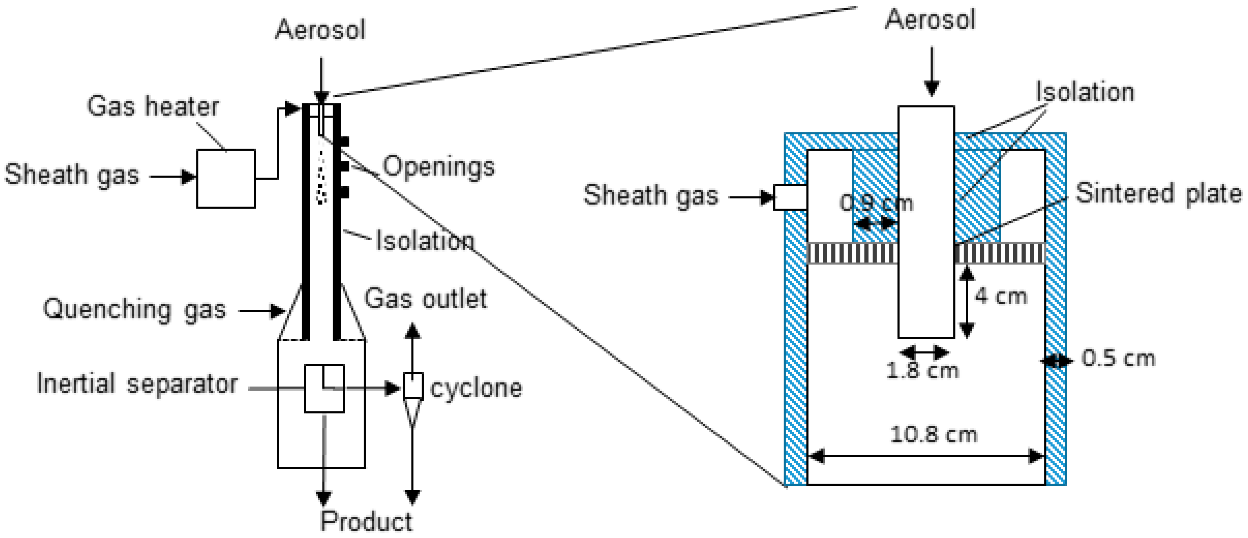
2.1. Rounding Setup

The rounding setup is composed of an aerosol generator unit, a gas heater, a downer reactor with a cooling section at the lower end of the pipe, and a separation system to recover the rounded particles as shown in Figure 1.
The aerosol dispersion unit consists of flat-tray feeder (ZD 22 FB-C-2M, Three-tec GmbH, Germany) which feeds the powders into a funnel connected with the suction orifice of a self-made powder Venturi injector. The rotatory velocity of the screws can be varied. The mass flow of PP particles was previously determined by measuring the mass of material collected as a function of time for each rotatory velocity of the screws. The nitrogen pressure in the Venturi injector controls the mass flow rate of aerosol gas.
A nitrogen sheath flow was heated employing a gas heater (GA00565, Horst GmbH, Lorsch, Germany). To reduce the heat losses, the pipe connecting the outlet of the gas heater with the inlet of the sheath gas was heated by using a heating band (HBS, Horst GmbH, Germany) wrapped around the pipe and was isolated using glass fabric tape. The mass flow of the sheath gas was controlled by a mass flow controller (EL-Flow, Wagner Mess-und Regeltechnik, Germany). To avoid the particles to melt in the aerosol nozzle due to the hot sheath gas, the aerosol nozzle is isolated from the sheath gas with a 9 mm thick layer of glass wool inside the head of the downer (see Figure 1).
The downer reactor is a stainless-steel pipe of a length of 80 cm and an inner diameter of 10.8 cm. In the downer, the particles are heated directly by the sheath gas. The outer walls of the downer (head, main pipe and flanges) were isolated by a 5 mm-thick layer of glass wool. The glass wool isolation was covered with aluminum foil. At the bottom of the downer, the diameter of the pipe is suddenly increased up to an inner diameter of 19 cm to reduce the velocity of the particles. At this section, air at room temperature was fed at a volume flow of 5 kg/h to cool down the particles. The outlet of the cooling section is oriented upwards (45° of inclination) at one side of the cooling section, such that most of the particles are separated by inertia due to the sudden change of stream direction and low particle velocity. The remaining gas-borne particles (fine particles) were separated from the gas phase in a cyclone.
For the experiments, PP powder (Coathylene® PD0580, Axalta Polymer Powders, Switzerland) was processed in the rounding reactor. The most important properties of the material were determined in previous investigations [31] and are listed in Table 1.
To investigate the influence of the process parameters on the performance of the process and particle properties (e.g., shape and size), the mass flow of powder, the temperature and the mass flows of sheath and aerosol gas were varied. The different operating points are summarized in the experimental matrix in Table 2.
The cross-section-averaged solids volume fraction at the aerosol inlet is calculated according to Equation (1):
( 1 ε ) a v , a e r = m ˙ p a r t i c l e s ρ p a r t i c l e s m ˙ p a r t i c l e s ρ p a r t i c l e s + m ˙ aerosol   ρ g a s
where ρ p a r t i c l e s and ρ g a s are the solid density and aerosol gas density at the experimetal conditions. The values of (1 − ε)av,aer for the different parameter sets are also reported in Table 2.

2.2. Particle Characterization

2.2.1. Scanning Electron Microscopy

Particle shape and surface morphology were characterized by scanning electron microscopy (SEM). A Gemini Ultra 55 (Zeiss, Jena, Germany) was used to take images of the rounded particles using a SE2 detector at an acceleration voltage of 1 kV at magnifications of 100× and 200×.

2.2.2. Particle Sizing

Particle size distribution (PSD) was determined by laser diffraction (Mastersizer 2000, Malvern Panalytical GmbH, Kassel, Germany) according to ISO13320-1, using the dry dispersion unit Scirocco 2000 at 50% of the vibration amplitude of the feeding tray.

2.2.3. Light Microscopy

Light microscopy and digital image processing were used to determine the particle shape distribution of the raw and rounded powders. The description of the employed sample preparation and analysis methodologies can be found elsewhere [5]. The factors selected to describe the shape of the particles were the circularity and solidity defined according to Equations (2) and (3):
  C i r c u l a r i t y :   χ = 4 π A P
S o l i d i t y :   s = A C
where A and P are the measured projected area and perimeter of the particle, respectively. C is the areal convex hull, which represents the area enclosed by the convex hull of the outer contour of particles.
The circularity is a function of the particle aspect ratio and surface profile (e.g., sharp edges protuberances). Particles with an aspect ratio close to one, but with highly irregular surfaces (increased perimeter) would depict low values of circularity. Analogously, particles with regular smooth surfaces, but lower aspect ratio would have low circularity values. Spherical particles with rounded regular edges would have a circularity value of 1 [33]. The solidity describes solely the surface profile and is sensitive to particle concavities such as sinter necks. Particles with large number of concavities on the projected surface profiles show low values of solidity while perfectly spherical (convex) particles have a solidity of one. The analysis of circularity and solidity is useful to describe the process of shape transformation as it allows to discriminate the influence of the rounding process on the aspect ratio and morphological roughness of the particles.

2.3. Mathematical Model

2.3.1. Governing Equations

The temperature and flow fields of the gas phase and the polymer particles were modelled using a continuous Eulerian–Lagrangian approach implemented in the commercial software Ansys Fluent version 17.2. In the Eulerian–Lagrangian approach, the gas phase is treated as a continuous medium, in which fluid dynamics is described by solving the local averaged Navier–Stokes equations while the particles are tracked by solving the Newtonian motion equation for single particles. The maximum solids volume fraction in the downer, achieved directly at the inlet of the aerosol gas ranges between 9.24 × 10⁻⁵ and 5.4 × 10⁻⁴ for the different tested conditions. Under these conditions, particles could influence the turbulence of the flow [34]. Furthermore, for the desired analysis it is necessary to consider the heat transfer between the phases. To take into account the exchange of momentum and heat between the phases, a two-way coupling approach was employed. It was assumed that the particles are inert. The model equations are summarized in Appendix A.
The coaxial feeding of the aerosol and sheath gas in the downer produces a confined jet also referred to as Craya–Curtet jets. These kinds of jets have been addressed in different investigations and they are of relevance for certain industrial applications such as jet pumps or jet furnaces [35,36,37]. One of the main issues associated with these kinds of jets is the appearance of a region of reverse flow or recirculation as well as separation zones near the wall when the coaxial surrounding flow is sufficiently low. This effect was shown by Sachs et al. [25], who studied the particle aerodynamics in a wall-heated downer reactor with similar inlet geometry as the investigated one in the current work by means of CFD simulations. The appearance of the recirculation zone is characterized by a critical Craya–Curtet number Ctc [35]. The craya-Curtet number (Ct) is defined as the square root of the ratio of the momentum flux of the co-flowing stream (Jc) to that of the central jet (Jj) (Equation (4)) [38].
C t = J c J j
For Ct < Ctc a recirculation zone appears while for Ct > Ctc the recirculation region is not formed. The values of Ctc ranges between 0.65 and 0.77 [35,38]. The magnitude of the recirculation (e.g., length, velocity, turbulence) increases with decreasing Ct [35]. The appearance of this recirculation zone is not desired during the rounding of polymer particles as it would increase the turbulence and thus the probability of collision between polymer particles leading to more pronounced agglomeration [25]. The geometry of the inlet section of the downer and the experimental conditions reported in Table 2 were selected such that the lowest Ct number obtained was 0.65 (parameter set 9). Under these conditions, it is assumed that a recirculation region is not formed or at least only to a negligible extend.
The realizable k-ε turbulence model [39] was employed. The realizable k-ε model performs well predicting the expansion of round jets as is the case of the aerosol injection in the downer. It also provides a better prediction of the flow of moderate anisotropic flows such as adverse pressure gradients, separation and recirculation compared to the standard k-ε model [39]. This model is simpler, more stable, leads to good convergence during the coupled simulations and requires less computational cost compared to anisotropic turbulence models. The equations of the model are given by Equations (A1)–(A33) [39]. The near-wall region was resolved using the enhanced wall treatment which combines the two-layer model [40] with the enhanced wall functions [41]. In the Lagrangian–Eulerian approach, the particle trajectories are calculated by solving the Newtonian particle motion equation using the previously solved flow and turbulence fields such that the effect of the near-wall layer on the particles trajectories is also considered indirectly by using this wall functions.
For the calculation of the particle tracks, the disperse phase model (DPM) of Ansys Fluent was employed. Only the effect of the drag force on the equations of motion was considered. Forces such as virtual mass and pressure gradient force can be neglected due to the large density difference between the gas and the particles ( ρ ρ p <<1). Saffman’s lift, thermophoretic and Brownian forces were neglected as they are only relevant for submicron particles. The drag coefficient for non-spherical particles was calculated according to (Equation (A26)) proposed by Heider et al. [42], where the shape factor is the sphericity of the particles. The sphericity was approximated to be the volume-mean circularity of the untreated powder measured according to Section 2.2. A constant value of = 0.7 was assumed. The turbulence dispersion of the particles was modeled by the discrete random walk (DRW) model [43,44]. This involves a stochastic approach to estimate the dispersion of the particles by considering the possible interaction of the particles with the eddies. This model assumes that the gas phase fluctuations has an effect on the particles turbulent scattering at the beginning of the interaction time with the eddy along the particle’s trajectory. The particle trajectories are calculated integrating the motion equation (Equation (A23)) coupled with the turbulence model. Here the instantaneous gas velocity v is given by Equation (A13), where v ¯ is the average velocity of the continuous phase determined from the CFD model and v ( t ) is the instantaneous fluctuating velocity of the continuous phase. v ( t ) is calculated according to Equation (A14) and depends on a random number, which obeys a Gaussian distribution ( ζ ), and the solution of the turbulence kinetic energy k. The interaction time of the particles with the eddy is the minimum of the characteristic eddy lifetime (Equation (A15)) and the particle eddy crossing time (Equation (A29)). When this interaction time is reached during the integration of the Equation (A23), a new value of ζ is calculated and the process is repeated. To account for most realistic random effects of the turbulence on the particles, the eddy’s lifetime was calculated considering a uniformly distributed number at random ( r   ϵ [ 0 , 1 ] in Equation (A15)) and 5 possible particle trajectories were calculated for each parcel. A total of 10,000 (2000 parcels × 5 tries per parcel) particles trajectories were simulated which allow obtaining statistically representative results. The heat transfer coefficient between surrounding gas phase and particles was modeled according to the correlation developed by Ranz and Marshall [45] (Equation (A28)) for spherical particles.

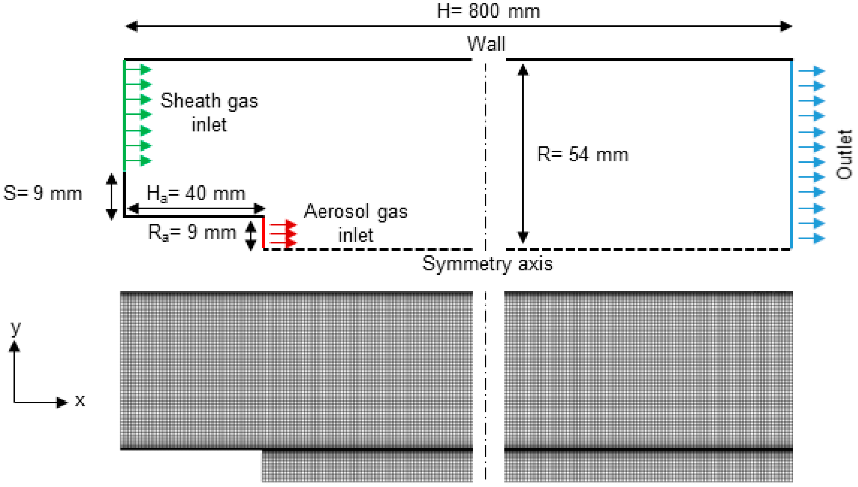
2.3.2. Computational Domain and Meshing

For the simulations only the pipe section between the sintered plate and the cooling section of the downer reactor was considered. In this case, gradients in the angular direction are considered to be negligible and the 3D simulation can be simplified by using a 2D axisymmetric domain [26]. The computational domain and the grid used for solving the simulations are shown in Figure 2.
A structured rectangular grid has been generated using the mesh module of Ansys such that aspect ratio of most of the cells is close to one. To capture the effect of the wall-boundary layer and the turbulence produced by the aerosol injection and jet expansion, the grid was refined in the near-wall regions and in the boundary region produced by extrapolating the end of the aerosol nozzle. The maximal element size is 1 mm × 1 mm in the axial and radial direction, respectively. The aforementioned conditions resulted in a total of 57,000 elements. The mesh-independency was tested using different mesh configurations (without refinement and the jet boundary layer) and different number of mesh elements. The results obtained with the described mesh delivered sufficient independency on the mesh size (see Appendix B.1).

2.3.3. Boundary Conditions and Material Properties

Figure 2 illustrates the boundary conditions of the problem and their location.
Gas phase:
The gas phase was assumed as only nitrogen (not considering the air suctioned by the Venturi injector). Properties such as density, viscosity, heat capacity and thermal conductivity were calculated for different temperatures at atmospheric pressure in the range of 20–500 °C using the NIST database [46]. The values of the properties were fitted to polynomial functions of fourth order as a function of temperature. The coefficients of the polynomial functions were given as parameter for the definition of the material properties in the simulations.
The inlet of the aerosol and sheath flow were modelled by velocity inlet condition with user-defined axial velocity and temperature profiles. This was defined in a way that makes the simulations more realistic, as the temperature and velocity profiles of aerosol and sheath gas are not uniform, but are already partially developed. The radial component of velocity was assumed to be 0 m/s.
The shape of the user-defined inlet axial velocity and temperatures profiles were approximated by the results of two pre-simulations. In these pre-simulations, the flow through the aerosol pipe and the annular region in the case of sheath gas were simulated assuming a pipe length of 1 m. For the pre-simulations, the meshing was set in a way that it perfectly fits the meshing of the inlets’ boundaries of the main simulation. The same models and solution approach of the main simulation were applied for the pre-simulations. Mass flow inlets of 8.9 kg/h (210 °C) and 1.35 kg/h (20 °C) were used as inlets for the pre-simulations of the sheath gas annular section and aerosol pipe, respectively. In both cases, the pressure outlet was used as boundary condition. For the pre-simulation of the flow in the aerosol nozzle, a constant heat flux of 100 W/m2 from the walls to the fluid was considered as the aerosol is heated by the heat transferred from the sheath gas to the isolation. For the pre-simulation of the sheath gas in the annular section, constant heat fluxes of −100 W/m2 and −376 W/m2 were assumed for the boundaries representing the aerosol isolation and the outer wall of the downer, respectively. These heat fluxes were determined from experimental measurements, as explained in Appendix B.2.
The outlet axial velocities and temperature radial distributions of the pre-simulations were exported, and their shapes were used as base for the generation of user-defined profiles for the main simulations. The radial temperature profiles from the pre-simulations were displaced towards higher or lower temperatures, such that the temperature at the center of the aerosol nozzle and the center of the annular section match the measured temperature at the same position for the different studied conditions. The procedure employed to measure these temperatures is described in Appendix B.2. The axial velocity profiles from the pre-simulations were multiplied by a factor such that the derived cross-section-averaged velocity of the aerosol and sheath gas matches that of measurements. The last-mentioned velocity was calculated from the experimentally determined mass flows (Section 2.1) and the corresponding hydrodynamic diameters and average cross-section temperatures of the aerosol and sheath gas.
The experimentally determined cross-section-averaged velocities and measured temperatures used for derivation of the axial velocity and temperature radial profiles for the different parameter sets are reported in Table 3.
An example of the inlet radial profiles of the axial component of the velocity and temperature for the sheath and aerosol gas for the parameter set No.1 is shown in Figure 3. The shape of the profiles is the same, but the values of the axial velocity and temperature are changed to fulfill the experimental values for each parameter set as explained above. The turbulence parameters for the inlets were defined by the hydraulic diameters and turbulent intensities of 2% and 1% for the aerosol and sheath gas inlets, respectively.
For the outlet of the downer, a pressure boundary condition at atmospheric pressure was used. The hydraulic diameter and a turbulent intensity of 5% were used to define the turbulence parameter at the outlet. The center line of the downer was set as “axis” boundary conditions. All other boundaries were set to stationary wall boundary conditions with no slip condition, such that the velocity magnitude of the fluid at the wall is 0 m/s. For the line representing the outer wall of the downer a constant heat flux of −376 W/m2 was used. For the boundaries representing the sintered plate region without sheath gas fed and the aerosol pipe wall, the heat fluxes was assumed to be 0 W/m2 and 100 W/m2, respectively. The heat fluxes through the walls used in the pre- and main-simulations were determined experimentally and are explained in Appendix B.2.
Disperse phase:
The material properties of the disperse phase (PP), reported in Table 1, were assumed to be constant in the simulations. In the disperse phase model of Ansys Fluent, the total number of particles is discretized in parcels, which represent groups of particles with exactly the same attributes. In this way, it is possible to reduce the computational cost of the simulation.
The initial conditions of the disperse phase were defined in an injection file generated in Matlab, which contains the information about the position in injection (x, y, z), the velocity components at injection (u, v, w), the diameter and temperature of each parcel. Additionally, the injection file includes the mass flow rate of the parcel which is necessary for the coupled calculations. A total of 2000 parcels were injected at the aerosol inlet position. The parcels were injected at the opening of the aerosol nozzle at axial position of x = 0.04 m. It was assumed that the parcels were randomly injected across the cross-section. The y and z coordinates were determined by an algorithm, which generates randomly distributed points across the cross-section of the aerosol pipe (Ra = 0.009 m). The injection points of the particles used for the simulation are shown in Figure 4.
The axial component of the velocity and the temperature of the parcels was set to be the cross-section-averaged velocity and temperature of the aerosol gas, respectively. The other components of the velocity were set to 0 m/s.
To account for the effect of the particle size on the hydrodynamic of the particles, several particle diameters were analyzed in the simulations. The particle diameters of the parcels were selected such that it modeled the density volume-average particle size distribution of the PP determined experimentally. For that, the measured particle size distribution was discretized in size intervals. The number of parcels having a defined diameter N ( d p ) was calculated according to Equation (5).
N ( d p ) = R o u n d ( q 3 ( d p ) Δ d p N )
where q 3 ( d p ) is the measured density particle size distribution at the interval center x, Δ d p is the interval width and N is the total number of parcels. The function “Round” rounds the result to the nearest integer. By following this approach, the sum of N ( d p ) differs by a few parcels from N. Thus, some parcels were randomly removed or added such that the total number of parcels remains at N = 2000. Figure 5 illustrates the measured q 3 ( d p ) Δ d p and the number of parcels as a function of the particle size. The particle diameters were then randomly assigned to the different injection points shown in Figure 5.
The mass flow of the parcels was assumed to be particle size dependent and was calculated according to Equation (6).
m ˙ p a r c e l ( d p ) = q 3 ( d p ) Δ d p m ˙ p N ( x d p )
m ˙ p is the particle mass flow for each parameter set specified in Table 2.
Five possible particle trajectories (tries) were calculated for each injected parcel with the random walk model. Thus, a total of 10,000 possible parcels trajectories were tracked in the simulation. When using the calculation of multiple parcel trajectories, the mass and momentum of each injection point is divided automatically by the number of simulated tries [47]. The particles escape the downer at the outlet of the domain.

2.3.4. Numerical Solution

The pressure-velocity coupled SIMPLE algorithm was used to solve the Navier–Stokes equations. A second order upwind discretization scheme for interpolation of variables at the element faces were adopted. Gradients at the cell’s centroids were calculated using the least squares cell gradient scheme. Residuals of the continuous phase equations of 10−5 were used as convergence criteria of the simulations. The equations for the disperse phase were solved each 10 iterations of the continuous phase.

2.3.5. Post-Processing of the Particle Tracks

After convergence of the steady simulations, the particle tracks containing information of the position (x, y, z), velocity components, temperature, particle size of the parcels at each time step was exported and post-processed using a Matlab code. The particle tracks were analyzed for their residence time in the downer and the residence time distribution of the particles above the melting point at the different analyzed conditions. The last accounts for the effective rounding time in the downer.
To account for the particles, which adhere to the wall due to melting, it was assumed that all particles approaching the wall (r = 0.99R) at higher temperatures than the melting onset are trapped at the wall, such that these parcels were removed from the particle tracks file and, thus, not considered in the further analysis. With this purpose, all the particles, which satisfied Equation (7) at any time step, were removed from the analysis.
y 2 + z 2 + d p 2 0.99 R    &    T P c
where y and z are coordinates of the particle center, dp is the particle diameter, Tp particle temperature and Tm is the material melting onset.
Separately, each of the parcel tracks from injection until reactor outlet were treated such that the time steps were determined, at which the particle temperature was higher than the melting onset temperature of the material Tm. The melting onset of the material is considered as the limiting temperature, which defines whether shape modification process takes place or not. For the used PP, this temperature is 160 °C [31]. Under this temperature no melting of the material, and thus no-shape modification occurs. Above this temperature, melting starts and thus the process of shape modification can take place. The time steps at which the particle temperature was higher than the melting onset were added together for each parcel resulting in the effective rounding time. The effective rounding represents the time the particles spend in the downer which contributes to rounding. The resulting effective time distribution was determined from the different parcels.
The simulations were validated by measurements of the axial temperature distribution at the center of the reactor and measurements of the residence time distribution of the aerosol gas. A description of the setups used for the measurements of temperature and residence time can be found in Appendix B.2 and Appendix B.3, respectively. The results of the validation are presented in Appendix B.4.
The presented model is limited for solids concentration and flow anisotropy similar to the experimental conditions analyzed in this work. For operating conditions at very low Ct numbers and, thus, large recirculation regions and increased turbulence below aerosol injection, the use of an anisotropic turbulence model is recommended. For solids concentrations higher than 1 × 10⁻³, the use of a two-way coupling approach is not accurate and a four-way coupling (e.g., Lagrangian-DEM method or Eulerian–Eulerian approach) need to be considered [34]. A further limitation of the model is that it only considers a mean shape factor (sphericity) to determine the drag coefficient during the calculation of the particle trajectories. It does not allow considering the distribution of the particle shape, as would be case of real polydisperse powders, and it does not consider the change of the particle shape during the rounding process. The DPM model of Ansys is not able to consider the pronounced electrostatic forces produced by the electrostatic charging of the particles during dispersion, as observed during the experiments. Due to these limitations, deviations between the predicted and real particle trajectories, and thus, residence time distributions are expected.

3. Results and Discussion

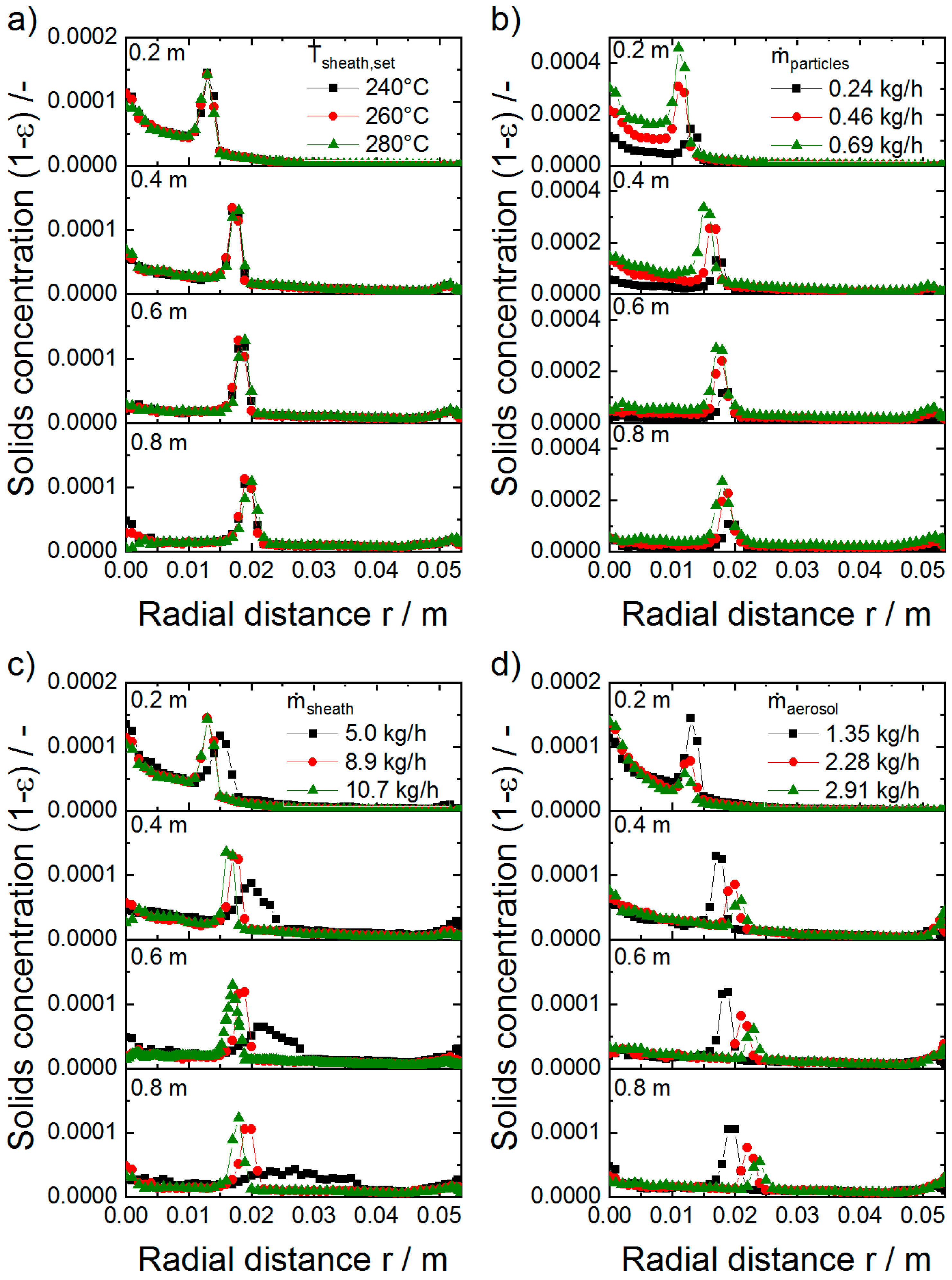
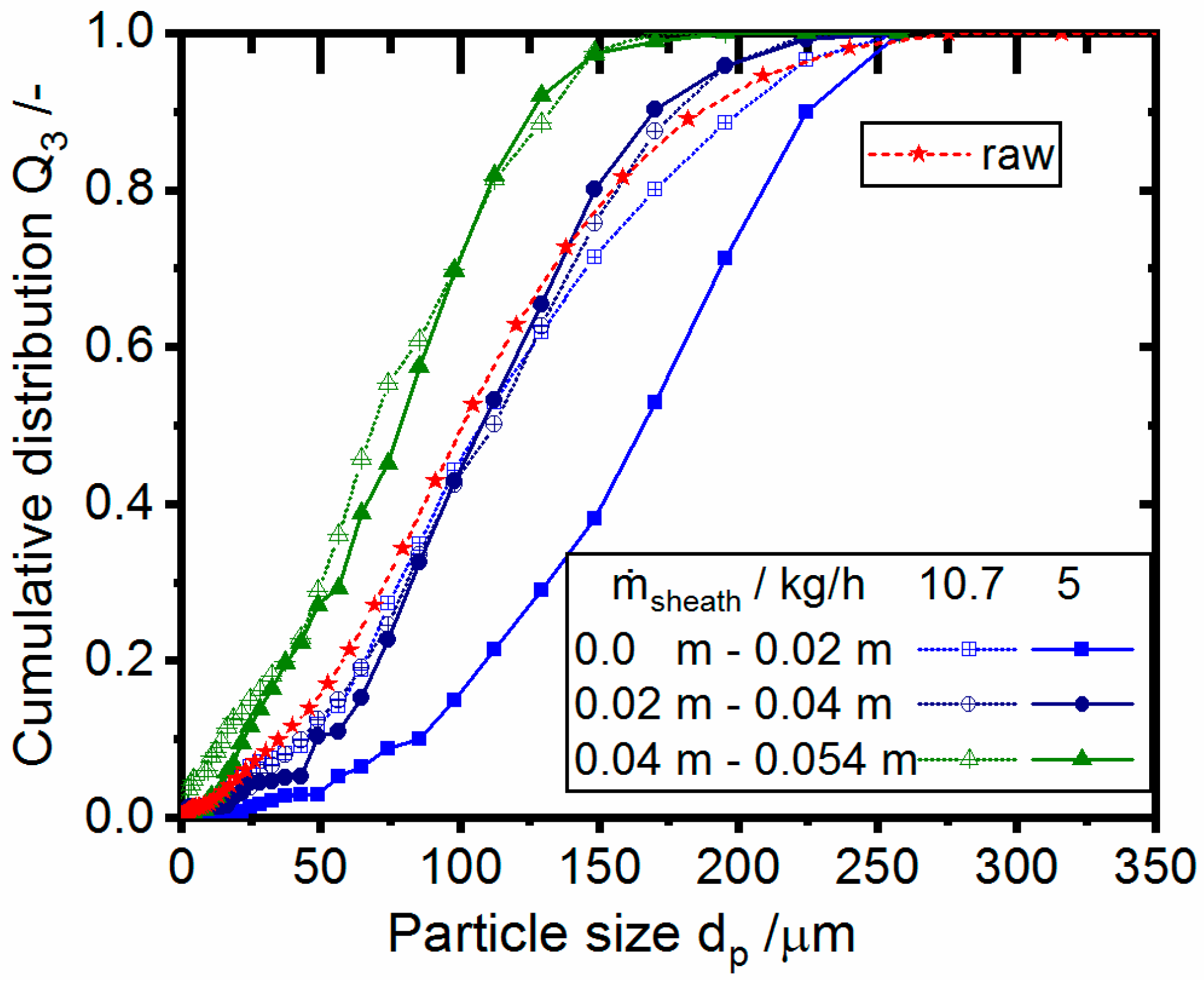
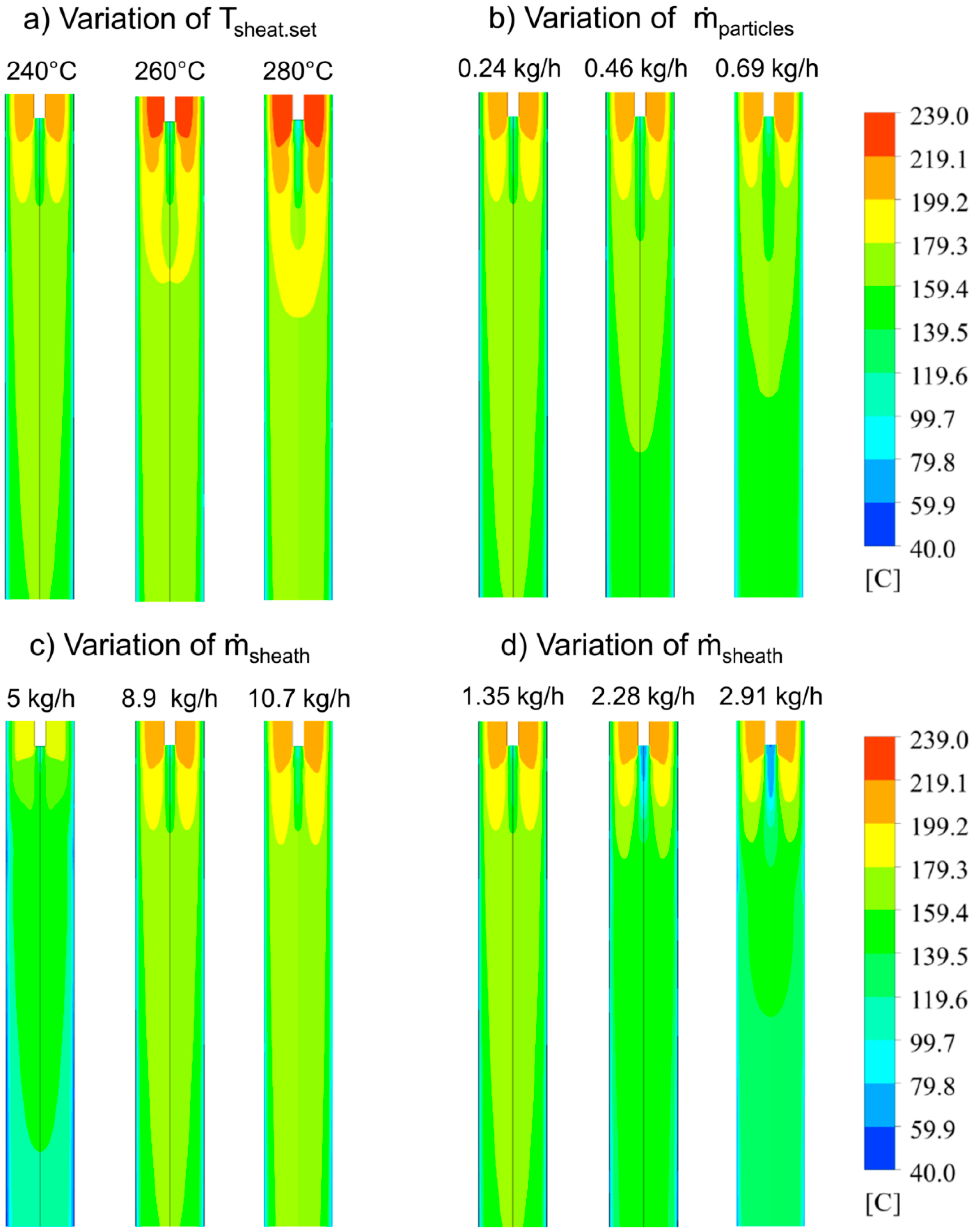
3.1. Effect of the Process Parameters on the Radial Solids Concentration in the Downer

Figure 6a–d shows the radial solids volume concentration profiles at different axial positions for the different cases studied. In all cases, two peaks of high solids concentration are observed at short axial distance after injection (x = 0.2 m): one at the axis (r = 0 m) and a second between r = 0.013 m–0.015 m. The peak at the axis decreases rapidly with increasing axial distance. The position of the second peak shifts towards the walls of the downer and the maximum of the peak decreases with increasing axial distance. At the same time, a smaller third peak is developed in the area close to the wall. The obtained solids concentration profiles differ significantly from the typical fully developed flow profile in downer reactors, where an almost uniform solids concentration in the core and a peak with high solids concentration near the wall region are observed. This is due to the inlet effects of the downer inlet geometry on the radial distribution of the particles, which are commonly observed after particle injection [27,48,49,50]. The observed profiles have similarities to those described by Cheng et al. [27] at the entrance region of a downer reactor with a similar single-jet solids injection system. The appearance of the second peak is explained by the accumulation of particles at the shear layer between the aerosol gas and the sheath gas observed in particle laden jet with coaxial containment gas [51]. The higher the ratio of mass flow of aerosol to sheath gas, the lower the height is and the faster the decrease of the second peak. This indicates a faster particle distribution through the cross-section of the downer.
Particle segregation can occur when using particle-laden jets. Bigger particles concentrate predominantly at the axis of the jet due to their higher inertia, while smaller particles drift mainly towards the wall driven by turbophoresis and tend to concentrate at the edge of the jet [51]. This fact was demonstrated experimentally by Sachs et al. [25], who investigated the size distribution of particles collected at different radial positions at the outlet of a 6 m-long downer reactor with a similar aerosol injection as in the present study. Particle segregation was also captured in the simulations by analyzing the size distribution of particles leaving the downer at different radial regions (0 m–0.02 m, 0.02 m–0.04 m and 0.04 m–0.054 m). This analysis is depicted in Figure 7 for the two extreme cases of Figure 6c (ṁsheath = 5.0 kg/h and ṁsheath = 10.7 kg/h). Here it is possible to observe that at the center of the downer the particle size shifted towards larger sizes with respect of the initial particle size distribution, while in the near wall region the size distribution shifted toward smaller particles.
According to Figure 6a, the set temperature of the sheath gas has no effect on the distribution of the particles in the downer. As observed in Figure 8b, the increase of the mass rate of particles produced a considerably increase of the solids holdup over the whole cross-section. It also has a small effect on the shape of the solids concentration profiles: the position of the second peak is slightly shifted toward the axis with increasing mass flow rate of solids. This effect is explained by the reduction of the jet expansion as consequence of the increment of the load of particles observed in particle laden jets [52].
The process parameters that influence the radial solids concentration profiles most are the mass flow of sheath and aerosol gas. When increasing the sheath gas flow rate for a constant gas flow, the expansion of the jet is reduced, resulting in a reduced particle dispersion. This effect is displayed by the displacement of the position of the second peak towards the downer axis as well as by the increase of its maximum (Figure 6c) and is more clearly seen for axial distances larger than 0.4 m. The decrease of the mass flow of sheath gas for a constant aerosol gas mass flow also leads to more pronounced particle segregation as observed in Figure 8. The opposite effects are observed when increasing the mass flow of the aerosol gas for a constant sheath gas mass flow. As observed in Figure 6d, this leads to an increase of the particle dispersion towards the wall and a pronounced particle segregation. Particle dispersion and segregation in the downer are then a function of the ratio of mass flows of aerosol and sheath gas. The higher this ratio, the more pronounced these effects are.

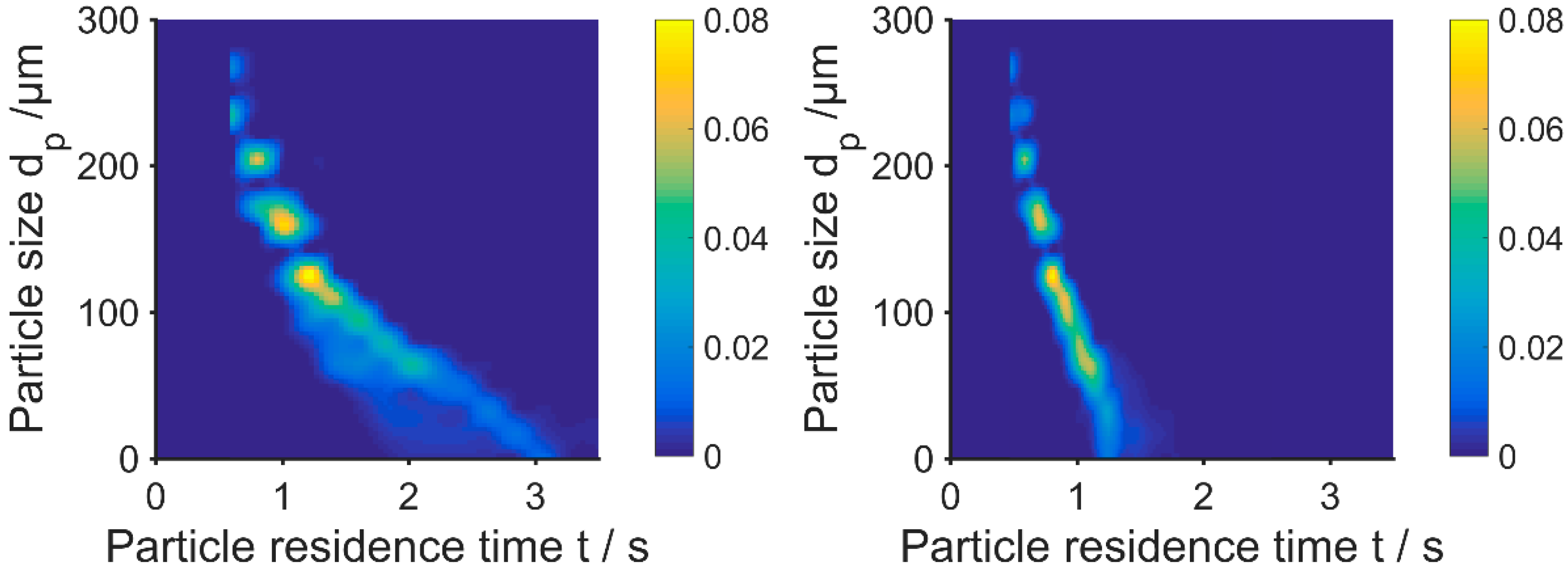
3.2. Influence of Process Parameters on the Particle Residence Time

The cumulative residence time distribution of particles (RTD) for the same parameter sets analyzed in Table 1 are shown in Figure 8a–d. As the number-averaged particle size distribution of the parcels in the simulation was derived from the measured volume-averaged particle size distribution of the powders, the calculated number-averaged residence time distributions in the simulations represent the expected real volume-averaged residence time distribution of the particles in the reactor. This residence time represents the total time that the particles spend in the downer, regardless of whether the particles melted or not. The mean residence time of the particles, the standard deviation and skewness of the distributions for the different cases are reported in Table 4.
As observed in Figure 8a, the variation of the sheath gas set temperature while keeping other parameters constant has a negligible effect on the residence time distribution of the particles. Neither the mean residence time, the standard deviation nor the skewness were affected significantly. A slight influence of the mass flow of particles on the residence time of the particles can be noticed in Figure 8b. Here the increase of the mass flow of particles from 0.24 kg/h to 0.69 kg/h causes a slight displacement of the particle residence time towards shorter values accompanied by a small increase of the broadness (standard deviation) and the skewness of the distribution (tail at larger residence times). As explained in Section 3.1, the increase of the particle mass flow rate leads to a reduction of the particle dispersion towards the wall, such that the particles concentrate in the core region of the downer. Since the axial velocities of the particles in the core region are larger relative to the regions near the wall, this leads to a shift in the RTD distribution of the particles toward short times when increasing the mass flow of particles.
More pronounced effects on the particle residence distribution are observed in Figure 8c,d due to changes in the mass flow rates of sheath gas and aerosol gas. In both cases, increasing the sheath gas flow or the aerosol gas flow contributes to a reduction of the residence time of the particles in the downer. The increase of either sheath gas flow or aerosol mass flow leads to a larger total gas flow rate in the downer and thus to larger axial velocities of both the gas and particles. The increase of the axial velocity of the particles leads then to shorter residence times. The broadness and skewness of the distributions are affected in opposite directions when increasing the flow rate of sheath and aerosol gas. When the flow of sheath gas is increased for constant flow of aerosol gas (Figure 8c), the broadness and the skewness of the RTD decreases significantly resulting in more homogeneous residence time distribution of the particles. In the other case (Figure 8d), the increase of the mass flow of aerosol gas for a constant mass flow of sheath gas leads to an increase of the tail at longer residence times and the broadness of the distributions (increased skewness and standard deviation), and thus, to less homogeneous particle residence time distributions. These effects are assumed to be related to the reduction or increase of the particle dispersion with the increase or decrease of the sheath gas flow rate with respect to the aerosol gas flow rate as explained in Section 3.1. The larger the particle dispersion towards the wall, the broader and the more asymmetric the distribution of residence time will be.
Clear correlations between the particle size and the particle residence time can be also established from the simulations results. Figure 9 shows the bivariate density distribution of the particle residence time and particle size for the two extreme cases of Figure 8c corresponding to the parameter sets 6 and 7 in Table 1. In both cases, it is observed that large particles (e.g., dp > 200 µm) spent considerable shorter time in the reactor compared with the small particles (e.g., dp < 50 µm). This is explained by the difference of mass, and thus, sedimentation velocity of the particle in the downer. A second observation is that the smaller the particle size, the broader the RTD. Due to the higher inertia of the large particles, they are less influenced by flow and will follow a straighter path towards the outlet of the downer. In contrast to that, small particles (e.g., dp < 50 µm) are more prone to be affected by the inlet effects which results in increased particle dispersion towards the wall of the downer and thus in a broader RTD.

3.3. Influence of Process Parameters on Temperature Distribution and Effective Rounding Time

The temperature distributions in the downer for different parameter sets are shown in Figure 10. The volume of the regions where the temperature is higher than the melting onset is referred in this work as effective rounding volume as only in these regions can the rounding take place. The time spent by the particles in the effective rounding volume is referred as effective rounding time. Figure 11 shows the cumulative distribution of effective particle rounding time for the same analyzed cases as in Figure 6, Figure 7, Figure 8, Figure 9 and Figure 10. Table 5 summarizes, the median (tr,50) and the 99th percentile (tr,99) of the effective rounding time distributions presented in Figure 11. As expected, a clear correlation between the effective rounding volume (Figure 10) and the effective rounding time can be observed. The larger the effective rounding volume, the longer the effective rounding time. In all the cases, the effective rounding time is always lower than the corresponding residence time, which is due to the fact that effective rounding volume is smaller than the reactor volume. Particles spend time in regions with temperatures below the melting onset (e.g., aerosol inlet and near-wall region), in which the particles “spend” time, which is not effective for rounding. In the ideal case, if the temperatures are higher than Tm in the whole downer volume, the effective rounding time distributions would equal the residence time distribution.
For all the examined parameter sets, a zone of relative low temperatures is observed directly after the injection of the particles. This is due to the colder temperature of the aerosol in comparison with the sheath gas temperature. For each axial position, the temperature decreases towards the downer walls.
Figure 10a shows the influence of the sheath gas set temperature on the temperature field in the downer when all the other parameters were left constant. Increasing the set sheath gas set temperature causes an expected overall increase of the temperatures in the downer as the total energy input into the system is increased. This leads to an increase of the effective rounding volume of the downer. According to Figure 11a, the increase of the set temperature of sheath gas from 240 °C to 260 °C leads to an increase of the effective rounding time in the downer. A further increase to 280 °C does not contribute to an increase of the effective rounding time since the effective rounding volume increases only slightly when the temperature is increased from 260 °C to 280 °C (Figure 10a).
As Figure 10b indicates, the global temperatures in the downer decrease when the mass flow of particles increases when all the other parameters are left constant. The higher the mass flow of particles the more energy is transferred from the gas phase to heat the solid phase, thus resulting in lower temperatures. As observed in Figure 10b, the mass flow of particles can, depending of the combination of parameters, influence significantly the regions of the downer where rounding takes place. By increasing the mass flow of particles from 0.24 kg/h to 0.69 kg/h, a decrease of the effective rounding time by above the half as observed in Figure 11b. This is due to the decrease of the temperatures and thus reduction of the effective rounding volume (Figure 10b).
The increase of the mass flow rate of sheath gas results in an increase of the energy input into the system and thus in an increase in the global temperatures in the downer. This is clearly observed in Figure 10c. For a mass flow sheath gas of 5 kg/h there is only a small annular region below particle injection, where the temperatures exceed the melting onset of PP such that only a reduced rounding effect is expected for this parameter set. When increasing the flow of sheath gas, the temperatures and thus the effective rounding volume of the reactor increases. A further increase of the flow rate of sheath gas higher than 10.7 kg/h would lead to an increase of the global temperatures in the downer but not lead to an increase of the effective rounding volume which is already approx. the reactor volume (with exception of the near wall region and immediate region after aerosol injection). The increase of the flow rate of sheath gas then leads to an increase of the effective rounding time in the first steps due to the increase of the effective rounding volume. This is evident in Figure 11c, where the increase of mass flow of sheath gas from 5 kg/h to 8.9 kg/h leads to an increase of the median effective rounding time from 0 s to 0.616 s. This effect decreases with the increase of flow rate: the increase from 8.9 kg/h to 10.7 kg/h only affects the effective rounding time distribution slightly. For ṁsheath > 10.7 kg/h, a further increase in the sheath gas flow rate will not result in a further increase in the rounding volume, but in a reduction in the residence time of the particles due to a shorter residence time as discussed in Section 3.2. The latter would in turn cause a reduction in the effective rounding time.
As the aerosol gas is only heated by the heat exchange between sheath gas and aerosol gas through the isolated aerosol pipe walls (see Figure 1), an increase of the mass flow of aerosol gas would lead to a decrease of the injection temperature of the aerosol. These two effects (increased aerosol gas total flow rate and decreased aerosol inlet temperature) cause a considerable reduction of the global temperatures in the downer as shown in Figure 10d. Here it can be seen that for the used parameters almost no rounding effects are expected for ṁaerosol ≥ 2.28 kg/h. Figure 11d shows that the increase of the mass flow of aerosol gas leads to a decrease of the effective rounding time due to the lower global temperatures in the downer and thus smaller rounding volume.
The simulation results also show clear dependences between the size and the effective particle rounding of the particles. Figure 12 shows the bivariate density distribution of the particle size and effective rounding time for the extreme cases of Figure 11b, where the variation of mass flow of particles was analyzed. The density distribution was determined considering only the particles that reached temperatures higher that the melting onset at some point of their trajectories.
For both cases, the reached effective rounding times and width of the distribution for a given particle size increases as the particle size decreases. This is due to the same reasons given when analyzing the dependences of residence time and particle size. As consequence, regardless of the parameters used, more pronounced rounding effects are expected to be observed in the small particles than the big ones. The comparison of the data in Figure 12 with the values reported for the corresponding case in Table 5 shows that tr,99 represents approximately the maximum effective rounding time achieved by the smallest particles (dp < 10 µm), while the median tr,50 represent nearly the mean effective rounding time of particle of sizes between 130 µm.
The comparison shown in Figure 13 also indicates that the maximum particle size that can be affected by the rounding process depends strongly on the set of parameters used: e.g., when using the process parameters of Figure 13 left, particles up to a size of approx. 250 µm are affected at some degree by the rounding process. However, if the parameter set of Figure 13 right are used the maximum particle size that can rounded reduced to approx. 180 µm.

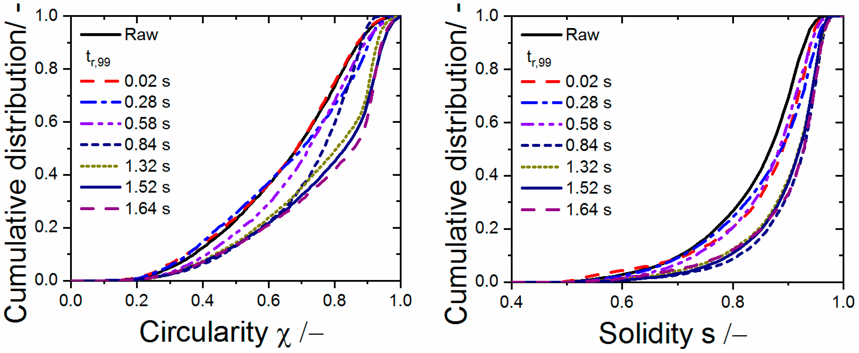
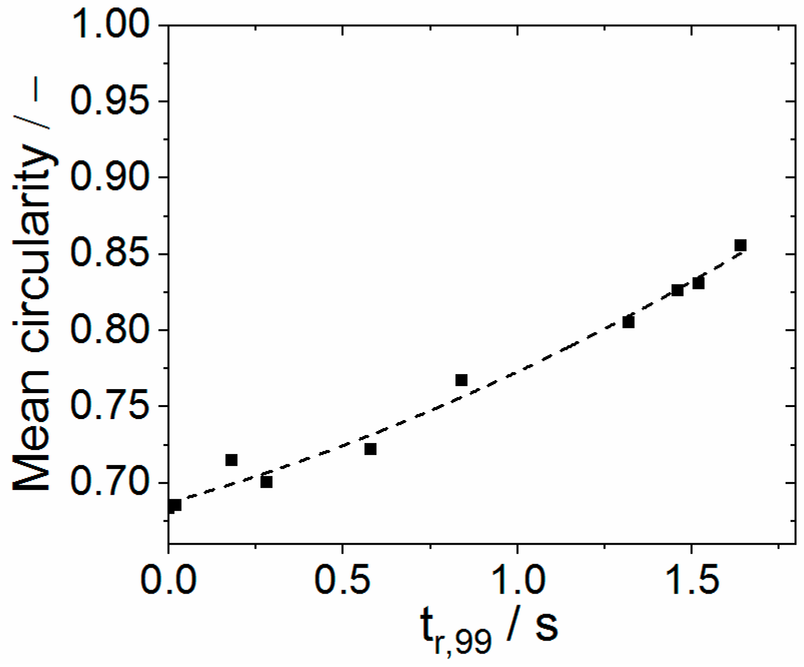
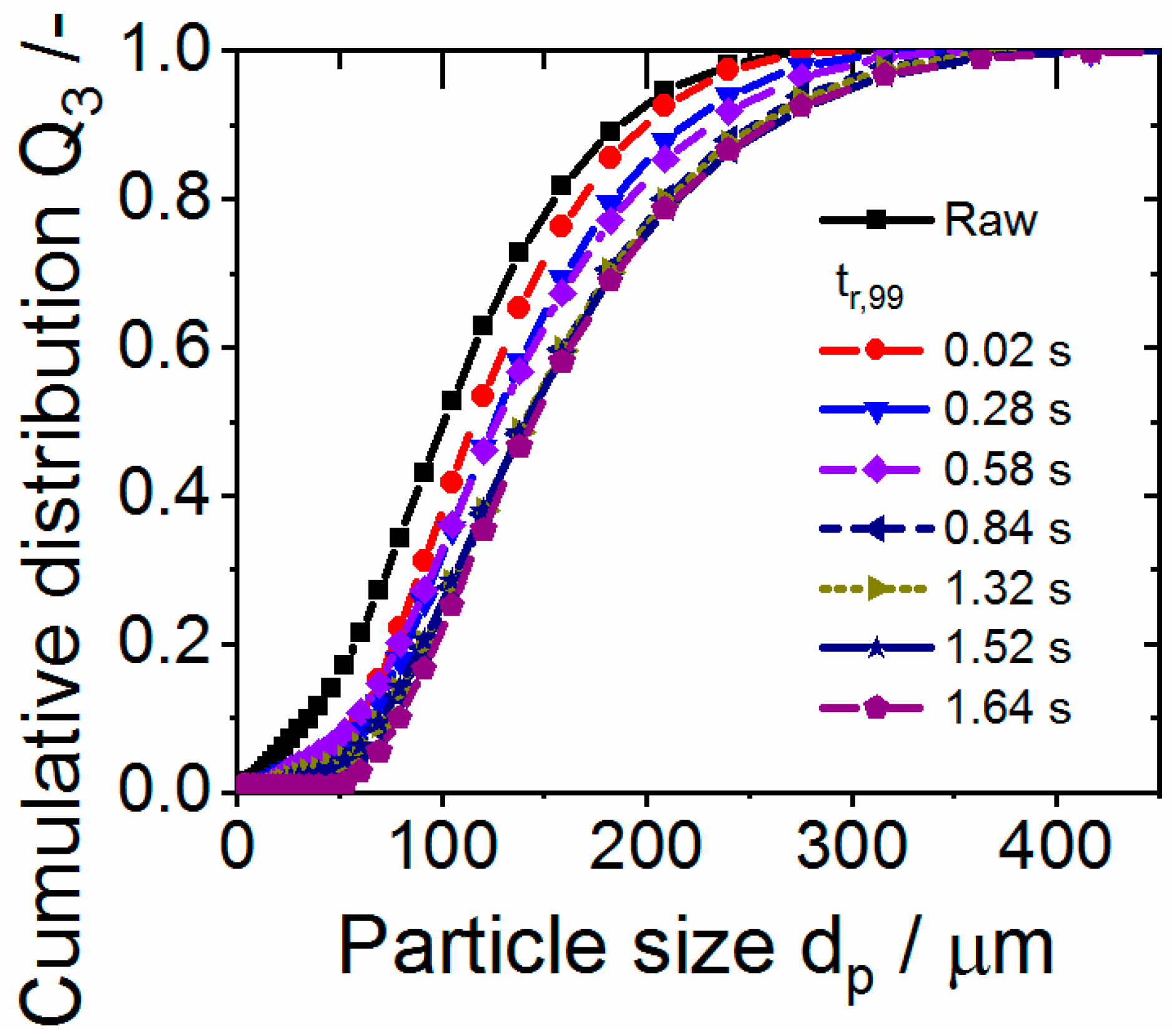
3.4. Effect of the Effective Rounding Time on Powder Properties

In the following section, the results of the rounding experiments for the different tested parameter will be presented. The results will be analyzed as a function of the effective rounding time obtained for each parameter set. This variable is the one that directly defines the rounding process and can be used to describe their progress. Figure 13 shows SEM images of the powder particles for the different tested conditions and Figure 14 shows the circularity and solidity distributions determined by light microscopy for some of the cases. In all the cases, the results were sorted as function of tr,99. As the tr,99 increases, shape modification proceeds. Both circularity and solidity increase progressively with increasing tr,99.
At the first steps of the rounding process the surface of the particles is mainly affected, i.e., protuberances and sharp edges become rounded resulting in smooth ellipsoidal particles. The latter become progressively more spherical with increasing rounding time. At tr,99 < 0.02 s the effect of the rounding process is almost negligible for most of the particles but can be already observed in a few small particles. When tr,99 increases, the number and the size of particles affected by the rounding process increase. At a tr,99 = 0.84 s almost all the particles become affected by the process. This is also observed in the circularity and solidity distributions, where a considerable change of the shape of the distributions is observed in comparison to those obtained for shorter tr,99. For longer effective rounding times the shape of the bigger particle continues changing toward a spherical shape. No considerable differences in terms of solidity are observed for the samples treated with tr,99 > 1.32 s. The progression of the rounding process as a function of tr,99 can be clearly observed when plotting the mean sphericity of the particles rounded at the different process conditions as a function of tr,99 as shown in Figure 15.
The results show that at the tested conditions, an increase of the mean circularity with respect to the raw material of about 25% was achieved. However, a complete rounding of the powders (mean circularity = 1, mean solidity = 1) could not be reached under the tested conditions. One reason is the relative shorter effective rounding time of the big particles dp ≥ 130 µm and thus limited rounding that can be achieved in the downer for this class of particles [17]. A second reason is the process intrinsic aggregation of the particles as a consequence of collisions between melted or partially melted particles described in previous investigations [5,17,25]. This results in the production of bigger structures made of two or more particles in different states of sintering depending on the effective rounding time of the produced aggregates. The production of these structures with lower circularity and solidity decreases the overall rounding effect [5,17]. These structures can be observed in some of the SEM images in Figure 13. Aggregation takes place even at very short effective rounding times. Despite the described particle aggregation and incomplete rounding of some big particles the rounding process leads to an improvement of the flow behavior of the rounded powders [5,17].
The effect of the rounding process on the particle size distribution of the rounded powders is shown in Figure 16. Here it is possible to observed that particle size distribution of the rounded powders shifts towards bigger sizes with increasing tr,99 between 0.02 s and 0.84 s. For tr,99 > 0.84 s the particle size of the rounded powders did not further increase. The increase of the particle size is the result of the particle agglomeration explained above in combination with the segregation of particle sizes in the downer. The latter leads to a reduction of the fine fraction in the product as small particles are more prone to spread towards the wall and attach there due to electrostatic forces and melting. These two effects are favored by the configuration of sheath gas/aerosol inlet used due to the relative high solids concentration and turbulence near the outlet of the aerosol jet in combination with hot surrounding sheath gas at this position.

4. Conclusions

The solids concentration profiles obtained in the simulations revealed that inlet effects are observed along the entire length of the downer. Radial particle segregation by size was observed in the simulations which confirmed the experimental observations of previous investigations. The combination of polydisperse particle size distribution of the material and inlet effects resulted in broad particle residence time distributions. The smaller the ratio of mass flows (i.e., the larger the mass flow of sheath gas compared to the aerosol gas mass flow), the more controlled were the particle segregation and radial dispersion. This leads in turn to more homogenous particle residence time distributions.
Heat losses through the wall and the injection of cold aerosol gas led to inhomogeneous temperature distributions along the reactor. In general, parameter changes, which increase the energy input in the system (e.g., increasing Tsheath.set or ṁsheath), led to a global increase of the temperatures in the downer. The increase of the mass flow of particles or aerosol gas for constant Tsheath.set and ṁsheath led to a decrease of the temperatures in the downer. A characteristic parameter referred to as effective rounding time was introduced. The effective rounding time of the particles depends on the parameter set used and its resulting temperature distribution, the thermal properties of the material (i.e., melting onset) and on particle properties which influences particle motion (i.e., size and shape).
Clear correlations were observed between the effective rounding time determined from the simulations and experiments by using the same parameters. In general, the longer the effective rounding time the higher the circularity and smoother the surface of the rounded product. Small particles are affected by the rounding process more significantly due to the longer effective rounding times compared to big particles. Operating conditions were identified which led to a considerable increase of the circularity of the particles. The broad distributions of effective rounding times and particle aggregation during rounding resulted in distributions of circularity and solidity.
Better rounding results for the tested PP powder can be achieved by setting the combination of parameters or increasing the length of the downer to reach longer effective rounding times, such that big particles and the produced aggregates becomes more rounded. The modification of the solids/gas inlet to reduce particle concentration and turbulence at the inlet are options to attenuate the particle aggregation and segregation. New distributor designs will be tested for this purpose. In general, better results are expected for powders made of smaller particles with narrow size distributions as it would lead to longer a more homogenous treatment of the particles.

Author Contributions

J.S.G.B.: Conceptualization, methodology, formal analysis, investigation, writing—original draft, writing—review and editing. L.U.: formal analysis, investigation. J.S.: conceptualization, methodology, formal analysis, writing—original draft, writing—review and editing, project administration. W.P.: methodology, validation, resources, formal analysis. A.B.: conceptualization, methodology, validation, resources, writing original draft, writing—review and editing, project administration. All authors have read and agreed to the published version of the manuscript.

Funding

Funded by the Deutsche Forschungsgemeinschaft (DFG, German Research Foundation)—Project-ID 61375930—CRC 814 (Additive Manufacturing), Sub-Project A2. Financial support is gratefully acknowledged.

Institutional Review Board Statement

Not applicable.

Informed Consent Statement

Not applicable.

Data Availability Statement

The data presented in this study are available on request from the corresponding author. The data are not publicly available due to confidentiality.

Acknowledgments

We thank OpenAccess support by FAU.

Conflicts of Interest

The authors declare no conflict of interest. The funders had no role in the design of the study; in the collection, analyses, or interpretation of data; in the writing of the manuscript, or in the decision to publish the results.

Appendix A. Governing Equations

Gas phase (Continuous phase)
Mass conservation equation
ρ t + ρ v i x i = 0
Momentum conservation equation
( ρ v i ) t + ( ρ v i v j ) x i = p x i + ( σ ij + τ ij ) x i + ρ g i + F p
Turbulent kinetic energy
t ( ρ k ) + x j ( ρ ku j ) = x j [ ( μ + μ t σ k ) k x j ] + τ ij v i x j + G b ρ ε
Production of k due to buoyancy
G b = g i μ t ρ Pr t ρ x i
Dissipation rate equation of turbulent energy
t ( ρ ε ) + x j ( ρ ε u j ) = x j [ ( μ + μ t σ ε ) ε x j ] ρ c 2 ε 2 k + v ε
Viscous stress tensor equation
σ ij = 2 μ S ij dev
Turbulent stress tensor equation
τ ij = 2 μ t S ij dev 2 3 ρ k δ ij
Eddy viscosity equation
μ t = ρ C μ k 2 ε
with
C μ = 1 A 0 + A s k   U * ε ,   U * = S ij S ij Ω ij Ω ij ,   A s = 6   COS Φ
and
Φ = 1 3 cos 1 6   W ,   W = S ij S jk S ki   S   ˜ 3 ,   S ˜ = S ij S ij
Strain-rate tensor
S ij = ( v i x j + v j x i )
Deviatory part of the strain-rate tensor
S ij dev = 1 2 ( v i x j + v j x i 2 3 δ ij v k x k )
Rate of rotation tensor
Ω ij = 1 2 ( v i x j v j x i )
Realizable k-ε model constants
A = 4.04 ; C 2 = 1.9 ;   σ ε = 1.0 ;   σ k = 1.2   ;   Pr t = 0.85
Instantaneous gas velocity
v =   v ¯ + v ( t )
Velocity fluctuation
v ( t ) = ζ 2 k 3  
Characteristic lifetime of eddy
τ e = 0.15 k ε log ( r )  
Eddy length scale
L e = C μ 3 4 k 3 2 ε
Energy equation
( ρ E ) t + v i ( ρ E + p ) x i = k eff T x i + S h
Total energy equation
E = h p ρ + v 2 2
Sensible enthalpy
h = 298.15   K T C pgas dT
Effective thermal conductivity
k eff = k + k t
Turbulent thermal conductivity
k t = C pgas μ t Pr t
Heat source term
S h = S w + S p
Solid phase (disperse phase)
Particle force balance
du p dt = F D ( v u p ) + g ( ρ p ρ ) ρ p
Drag force per unit particle mass
F D ( v u p ) = 18 μ ρ p d p 2 C D Re 24 ( v u p )
Particle Reynolds number
Re = ρ d p | u p u | μ
Drag coefficient
C D = 24 Re ( 1 + b 1 Re b 2 ) + b 3 Re b 4 + Re b 1 = exp ( 2.3288 6.4581 + 2.4486 2 ,   b 2 = 0.0964 + 0.5565 b 3 = exp ( 4.905 13.8944 + 18.8944 2 10.2599 3 )   b 4 = exp ( 1.4681 + 12.2584 20.7322 2 15.8855 3 )
Energy balance
m p c p p dT p dt = hA p ( T T p )
Heat transfer coefficient
Nu = hd p k = 2.0 + 0.6   Re 0.5 Pr 1 3
Particle crossing time
t cross = τ ln [ 1 ( L e τ | u p u | ) ]  
Particle relaxation time
τ = ρ p d p 2 18 μ 24 C D R e
Interaction time of particle with eddy
Min ( τ e ,   t cross )
Coupling between discrete and continuous phases at each control volume (CV)
Momentum exchange
F p = 1 V CV i = 0 N c v F D , i ( u p , i v )   m ˙ p , i Δ t
Heat exchange
S p = 1 V CV i = 0 N c v   m ˙ p , i c p p , i Δ T p , i

Appendix B. Additional Experimental and Simulation Setup

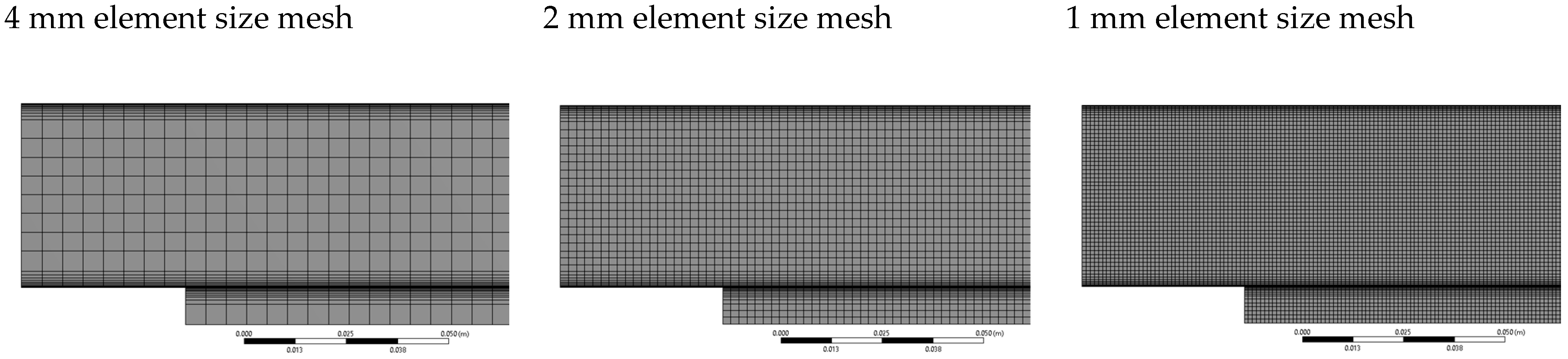
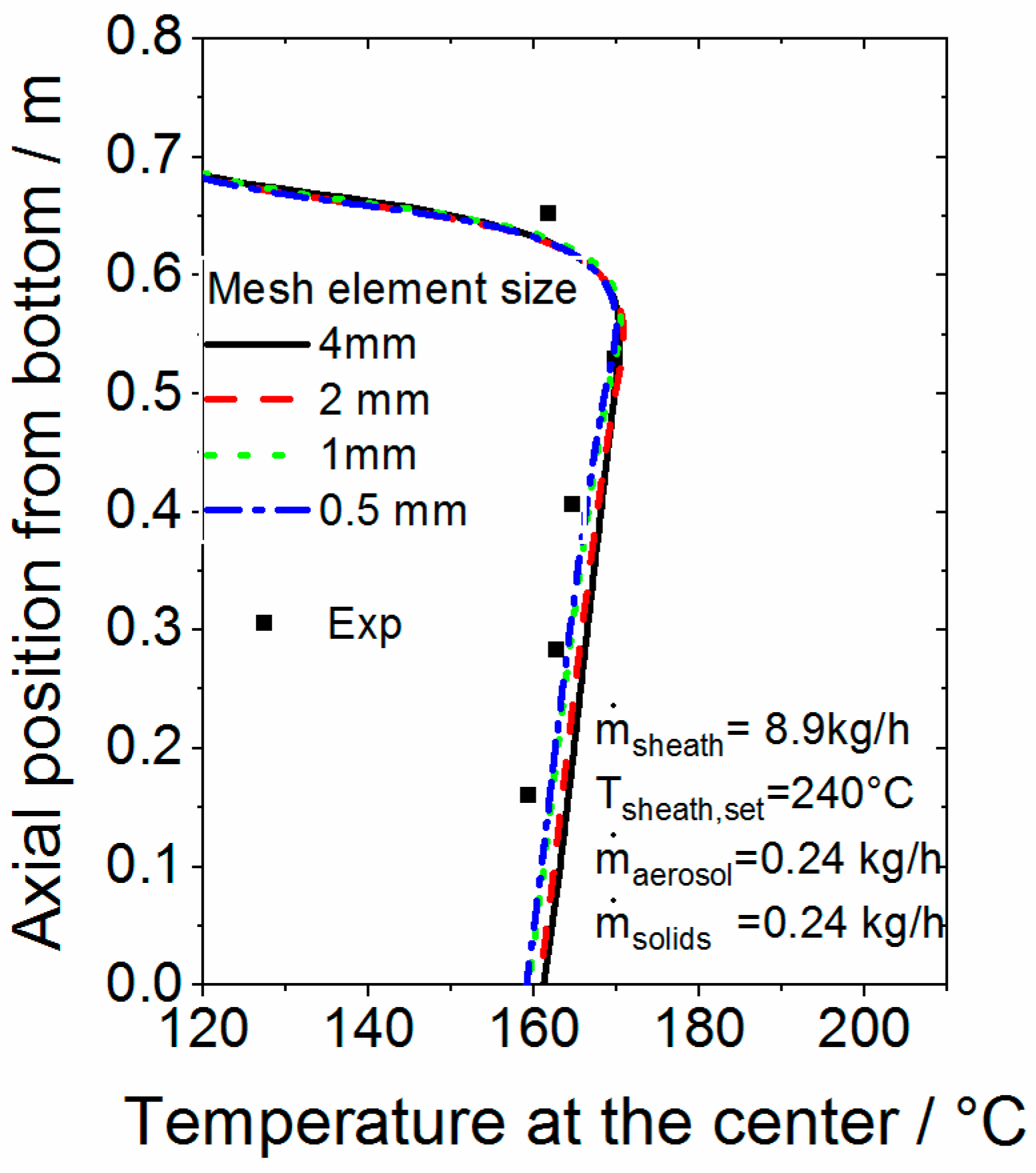
Appendix B.1. Mesh Independeny Study

We investigate the mesh independency by analyzing the axial temperature distribution at the center of the downer for different mesh configuration. We produce elements with the same size in the x and y direction with exception of the inflation regions. We variate the size of the elements between 4 mm, 2 mm, 1mm and 0.5 mm. Some example of the meshes used are depicted in Figure A1.
Figure A1. Example of three different meshes analyzed in the mesh independence study.
Processes 09 00916 g0a1
The results of the axial temperature distributions for the conditions of parameter Set 1 for the different meshes are shown in the Figure A2.
Figure A2. Axial temperature profiles at the center of the downer at the conditions of the parameter Set 1 calculated using different mesh sizes.
Processes 09 00916 g0a2
Reducing the mesh size from 1 mm to 0.5 mm, and thus, increasing the number of elements, did not produce significant changes in the calculated temperature profiles. That demonstrate that the results are mesh independent when using the 1 mm element size mesh. However, the increase of the number elements for the 0.5 mm mesh increases the computational time considerably. Thus, it was decided to use the 1 mm mesh size.

Appendix B.2. Setup for Temperature Measurements and Determination of Heat Fluxes through the Reactor Wall

With the aim of determine the heat fluxes through the different walls of the downer and obtain experimental data to validate the simulations, some measurements were conducted before the rounding experiments. Temperature measurements at different sections of the downer and measurements of the residence time distribution of a tracer gas fed in the aerosol gas were carried out. For these measurements, the cooling section, the stainless steel sheet and the separation units were removed and the reactor was operated without the additions of powder.
Five thermocouples (Type K, TC-Direct, Mönchengladbach, Germany) were inserted at different axial position in the openings of the downer pipe such that the tips of the thermocouples measured the temperature exactly at the axis of the reactor. The thermocouples were installed at 0.16 m, 0.28 m, 0.4 m, 0.53 m and 0.65 m from the bottom of the downer pipe. An additional thermocouple was fixed directly under the sintered plate at the center of the annular section to measure the sheath gas temperature at the inlet of the downer. The temperature at the center of the aerosol nozzle at the outlet was measured separately by fixing a thermocouple at this position. To have access to this section, the downer pipe was removed.
The measured temperatures were recorded using acquisition card (NI9213, National instruments, Austin, TX, USA). A LabView® Graphical program was used to monitor and record the results of the measurements. Temperature measurements revealed that a steady conditions was achieved at about 1.5 h after heating of sheath gas (initial temperature = room temperature). To facilitate the reproducibility of the results, all the measurements were recorded after 1.5 h preheating when it is in steady state. The reported values correspond to the mean value of temperature measured during 5 min. The axial temperature profiles upon the simultaneous injection of aerosol gas were used to validate the temperature field predicted by the simulations.
The thermal conditions at the different walls were approximated to have a constant heat flux surface. The heat flux through the wall and isolation of the downer were calculated from the axial temperature profiles when the aerosol nozzle was removed and the perforated sintered plate was replace by an unperforated plate. For a constant surface heat flux, the heat flow through the wall can be determined from Equation (A34) [53]:
q ˙ s , w a l l = m ˙ s h e a t h C p 2 π R d T d h
where d T d h is the slope of the measured axial temperature profiles and R is the inner radius of the downer pipe.
For the determination of the heat flux through the aerosol pipe and isolation a similar approach was employed. As the inlet temperature of the aerosol is room temperature and the temperature at the outlet at the center of aerosol pipe was measured, the heat flux through aerosol pipe wall q ˙ s , w a l l , a   can be calculated from Equation (A34), using = Δ T = T a e r o s o l T 0 , d h = L a , R = R a and m ˙ a e r o s o l instead of m ˙ s h e a t h . Where R a and L a inner radius and length of the aerosol nozzle, respectively.
The heat flux through the walls and isolation of the head of the downer was then approximated from the heat balance at this section according to Equation (A35).
q ˙ s , w a l l , h = ( m ˙ s h e a h t C p   ( T s h e a t h , i n t s h e a t h , d ) 2 π R a L a q ˙ s , w a l l   ) ( 2 π R L H + π R 2 )
where L H is the length of the cylindrical part of the downer head.
This procedure was applied for the different parameter sets in Table 2, which resulted in approximately similar values of heat fluxes. For that reason the mean value of the heat fluxes for the different conditions were used as constant values in the simulations.

Appendix B.3. Determination of the Residence Time Distribution of Aerosol Gas in the Downer

Appendix B.3.1. Measurement Setup

The measurement of residence time distribution of the aerosol gas in the downer using Helium (He) as a tracer gas. A mass spectrometer (Omnistar® GSD 300 O1, Pfeiffer Vacuum GmbH, Asslar, Germany) was used as detector by monitoring the ion current intensity of He+ (mass-charge ratio of m/z = 4) over time at two different positions. Position 1 was measured directly at the outlet of the aerosol nozzle at y = 0.76 m at the center of the reactor from the bottom of the downer, Position 2 was measured at the outlet y = 0 of the downer at the center. The ion current intensity at m/z = 4 was measured for 3 min each 0.25 s.
The schematic representation of the dosage system used to control the amount and duration of the He Feed is shown in Figure A3. The dosage of He was operated at pulses. A mass flow controller (MFC) (EL-Flow, Wagner Mess-und Regeltechnik, Offenbach am Main, Germany) was used to set the volume flow of He to 0.5 kg/h. A three-way-valve (6LVV-ALD3TC333P-C, Swagelok, Solon, OH, USA) with pneumatic control head and solenoid pilot valve was used to control the pulse time. When the three-way valve was actuated, Helium was conducted to the suction orifice of the venture injector. The actuation time of the valve was controlled by an output card (NI947299, National Instruments, Autin, TX, USA). A LabView® Graphical program was used to control the pulse time. The pulse time of He used for the validation experiments was set to 0.1 s.
Figure A3. Schematic representation of the tracer gas dosing system.
Processes 09 00916 g0a3
The structure of the sampling probe used for the measurements are shown schematically in Figure A4. A steel construction was fixed at the lower flange of the downer pipe which allow to fix the sampling probe at the axis of the downer and to displace the probe vertically at the desired measuring position. The probe is composed of the stainless steel pipe with a length of 1 m and inner and outer diameters of 5.7 and 8.3 mm, respectively. A stainless steel capillary of outer diameter of 2 mm a total length of 2 m is inserted into the stainless steel pipe. The capillary is connected directly at the mass spectrometer, which use vacuum to suction continuously the gas sample. The capillary is supported inside the pipe by two Teflon rings at both extremes of the stainless steel pipe. The function of the stainless steel pipe is to stabilize and protect the capillary.
Figure A4. Setup of the sampling probe.
Processes 09 00916 g0a4
As explained by Brust [48],the two-point measuring method allow the get rid of problems associated with the non-ideal Dirac function used and with the mixing effects in the capillary and mass spectrometer which overlaps with the reactor internal mixing effects. Thus, to investigate the residence time any input signal can be used, provided that the dosing process and the mixing behavior on the way to and in the detector is the same for the measurements at the two measuring positions. The residence time distribution of the aerosol gas in the downer E(t) is related to the input signal (X(t) at position (1) and output signal (Y(t) at position (2) according to the mathematical operation of convolution (Equation (A36)) [48,54]:
Y = E X
There are two possible way to determine the residence time distribution: the direct deconvolution of the Output and Input signals and adaptation of E(t) to the output function with by means of convolution. The first method is a numerically unstable process in which depending of the quality of the raw data may result in oscillations. Thus, leading to mathematical solutions with no physical sense [48]. For that reason, the convolution method was chosen for this investigation. This method requires to know a model representation for the E(t)-function. Since the downer is a tubular reactor, the analytical solution for the axial dispersion model [55] assuming an open-open system was used to modelling the residence time distribution in the downer E(t) (Equation (A37)).
E ( t ) = 1 2 u π   D a x t exp ( ( L u t ) 2 4   D a x t )
where the parameters u , L and D a x correspond to the superficial gas velocity, the length of the reactor and the axial dispersion coefficient, respectively.
To calculate the convolution of the convolution of the input signal with the modeled E ( t ) the so-called convolution integral (Equation (A38)) was used.
Y ( t ) = 0 t X ( t ) · E ( t t ) · d t
Thus, with an initial set of parameters u , L and D a x , a curve E(t) is calculated with Equation (A37). With the calculated E(t) an output curve is calculated with Equation (A38). Using minimization of the error square sums the corresponding model parameters can be determined by fitting the calculated output curve to the measured one. The raw data (ion current intensity vs. time) were based-line corrected and normalized such that area under the curve equals one, previous to the calculations. The data processing was implement in a Matlab® code.
Three measurements were carried at the two positions for each condition such that nine possible combinations of X and Y are possible. Unfortunately, no all the combination led to reasonable physical results.

Appendix B.3.2. Simulation of the Residence Time Distribution of the Aerosol Gas

The residence time distribution of the aerosol gas was calculated by transient flow simulations at different conditions upon the injection of a fictive tracer with exactly the same properties than nitrogen using the equations for the gas phase described in Table 2. The algorithm used for the determination of the residence time of the tracers gas from the CFD simulations was based on the procedure explained by Adeosun et al. [56]. In the first step, the flow, energy and turbulence equations were solved for the desired conditions in steady mode until fully convergence was achieved. In the next step, the species transport model of Fluent® was activated and the tracer gas was injected at the aerosol inlet at a mass fraction of one. The simulation was then conducted in the transient mode for 100 time steps of 0.01s, such that the tracer was injected for 0.1 s as in the experiments. After the injection of the tracer gas, the mass fraction of the tracer gas was set at zero. The simulations were then conducted for further 1000 time steps and the cross-sectional average molar concentration of tracer gas at the outlet was recorded over time. Upon normalization of the area under the obtained curve, the simulated density distribution of the aerosol gas E(t) was obtained. As in the experimental determination of the residence time distribution, no solids were injected in the simulations.

Appendix B.4. Validation Results

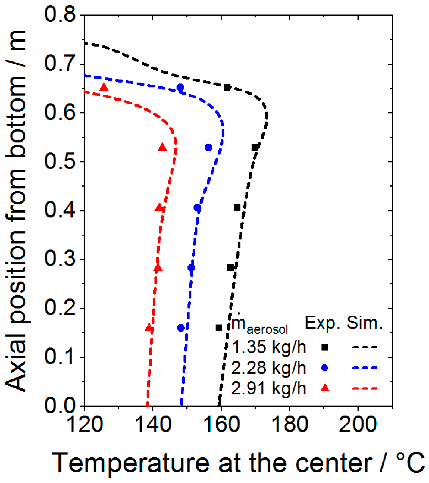
Appendix B.4.1 Axial Temperature Profiles (Figure A5)

Figure A5. Comparison of axial temperature profiles at the downer’s axis determined by experiments and simulations. (top) Variation of Tsheath,set with ṁsheath = 8.9 kg/h, ṁaerosol = 1.35 kg/h. (middle). Variation of ṁsheath with Tsheath.set = 240 °C, ṁaerosol = 1.35 kg/h; (bottom). Variation of ṁaerosol for Tsheath,set = 240 °C, ṁsheath = 8.9 kg/h.
Processes 09 00916 g0a5aProcesses 09 00916 g0a5b

Appendix B.4.2. Residence Time Distribution of Aerosol Gas (Figure A6)

Figure A6. Comparison of residence time distributions of the aerosol gas in the downer determined by experiments and simulations at different ṁaerosol at Tsheath,set = 240 °C and ṁsheath = 8.9 kg/h.
Processes 09 00916 g0a6aProcesses 09 00916 g0a6b

References

  1. Bahadur, S.; Badruddin, R. Erodent particle characterization and the effect of particle size and shape on erosion. Wear 1990, 138, 189–208. [Google Scholar] [CrossRef]
  2. Maile, F.J.; Pfaff, G.; Reynders, P. Effect pigments—Past, present and future. Prog. Org. Coat. 2005, 54, 150–163. [Google Scholar] [CrossRef]
  3. Podczeck, F.; Mia, Y. The influence of particle size and shape on the angle of internal friction and the flow factor of unlubricated and lubricated powders. Int. J. Pharm. 1996, 144, 187–194. [Google Scholar] [CrossRef]
  4. Fu, X.; Huck, D.; Makein, L.; Armstrong, B.; Willen, U.; Freeman, T. Effect of particle shape and size on flow properties of lactose powders. Particuology 2012, 10, 203–208. [Google Scholar] [CrossRef]
  5. Bonilla, J.S.G.; Dechet, M.A.; Schmidt, J.; Peukert, W.; Bück, A. Thermal rounding of micron-sized polymer particles in a downer reactor: Direct vs indirect heating. Rapid Prototyp. J. 2020, 26, 1637–1646. [Google Scholar] [CrossRef]
  6. Schmidt, J.; Sachs, M.; Blümel, C.; Winzer, B.; Toni, F.; Wirth, K.-E.; Peukert, W. A novel process route for the production of spherical LBM polymer powders with small size and good flowability. Powder Technol. 2014, 261, 78–86. [Google Scholar] [CrossRef]
  7. Otani, M.; Minoshima, H.; Ura, T.; Shinohara, K. Mechanism of particle shape modification by dry impact blending. Adv. Powder Technol. 1996, 7, 291–303. [Google Scholar] [CrossRef]
  8. Bissett, H.; van der Walt, I.; Havenga, J.; Nel, J. Titanium and zirconium metal powder spheroidization by thermal plasma processes. J. S. Afr. Inst. Min. Met. 2015, 115, 937–942. [Google Scholar] [CrossRef]
  9. Kotlyarov, V.I.; Beshkarev, V.T.; Kartsev, V.E.; Ivanov, V.V.; Gasanov, A.A.; Yuzhakova, E.A.; Samokhin, A.; Fadeev, A.A.; Alekseev, N.V.; Sinayskiy, M.A.; et al. Production of spherical powders on the basis of group IV metals for additive manufacturing. Inorg. Mater. Appl. Res. 2017, 8, 452–458. [Google Scholar] [CrossRef]
  10. Tang, J.; Nie, Y.; Lei, Q.; Li, Y. Characteristics and atomization behavior of Ti-6Al-4V powder produced by plasma rotating electrode process. Adv. Powder Technol. 2019, 30, 2330–2337. [Google Scholar] [CrossRef]
  11. Zhao, Y.; Cui, Y.; Numata, H.; Bian, H.; Wako, K.; Yamanaka, K.; Aoyagi, K.; Chiba, A. Centrifugal granulation behavior in metallic powder fabrication by plasma rotating electrode process. Sci. Rep. 2020, 10, 18446. [Google Scholar] [CrossRef]
  12. Jin, H.; Xu, L.; Hou, S. Preparation of spherical silica powder by oxygen–acetylene flame spheroidization process. J. Mater. Process. Technol. 2010, 210, 81–84. [Google Scholar] [CrossRef]
  13. Mys, N.; van de Sande, R.; Verberckmoes, A.; Cardon, L. Processing of Polysulfone to Free Flowing Powder by Mechanical Milling and Spray Drying Techniques for Use in Selective Laser Sintering. Polymers 2016, 8, 150. [Google Scholar] [CrossRef] [Green Version]
  14. Mys, N.; Verberckmoes, A.; Cardon, L. Processing of Syndiotactic Polystyrene to Microspheres for Part Manufacturing through Selective Laser Sintering. Polymers 2016, 8, 383. [Google Scholar] [CrossRef] [PubMed] [Green Version]
  15. Schmidt, J.; Sachs, M.; Fanselow, S.; Zhao, M.; Romeis, S.; Drummer, D.; Wirth, K.-E.; Peukert, W. Optimized polybutylene terephthalate powders for selective laser beam melting. Chem. Eng. Sci. 2016, 156, 1–10. [Google Scholar] [CrossRef]
  16. Dechet, M.A.; Gómez Bonilla, J.S.; Lanzl, L.; Drummer, D.; Bück, A.; Schmidt, J.; Peukert, W. Spherical Polybutylene Terephthalate (PBT)—Polycarbonate (PC) Blend Particles by Mechanical Alloying and Thermal Rounding. Polymers 2018, 10, 1373. [Google Scholar] [CrossRef] [Green Version]
  17. Gómez Bonilla, J.S.; Kletcher, R.; Lanyi, F.; Schubert, D.W.; Bück, A.; Schmidt, J.; Peukert, W. Effect of particle rounding on the processability of polypropylene powder and the mechanical properties of selective laser sintering produced parts. In Proceedings of the 30th Annual International Solid Freeform Fabrication Symposium, Austin, TX, USA, 12–14 August 2019. [Google Scholar]
  18. Kondo, K.; Kido, K.; Niwa, T. Spheronization mechanism of pharmaceutical material crystals processed by extremely high shearing force using a mechanical powder processor. Eur. J. Pharm. Biopharm. 2016, 107, 7–15. [Google Scholar] [CrossRef]
  19. Mundszinger, M.; Farsi, S.; Rapp, M.; Golla-Schindler, U.; Kaiser, U.; Wachtler, M. Morphology and texture of spheroidized natural and synthetic graphites. Carbon 2017, 111, 764–773. [Google Scholar] [CrossRef]
  20. Naito, M.; Kondo, A.; Yokoyama, T. Applications of comminution techniques for the surface modification of powder materials. ISIJ Int. 1993, 33, 915–924. [Google Scholar] [CrossRef] [Green Version]
  21. Murray, J.; Simonelli, M.; Speidel, A.; Grant, D.; Clare, A. Spheroidisation of metal powder by pulsed electron beam irradiation. Powder Technol. 2019, 350, 100–106. [Google Scholar] [CrossRef]
  22. Zhu, J.-X.; Yu, Z.-Q.; Jin, Y.; Grace, J.R.; Issangya, A. Cocurrent downflow circulating fluidized bed (downer) reactors —A state of the art review. Can. J. Chem. Eng. 1995, 73, 662–677. [Google Scholar] [CrossRef]
  23. Cheng, Y.; Wu, C.; Zhu, J.; Wei, F.; Jin, Y. Downer reactor: From fundamental study to industrial application. Powder Technol. 2008, 183, 364–384. [Google Scholar] [CrossRef]
  24. Lehner, P.; Wirth, K.-E. Characterization of the flow pattern in a downer reactor. Chem. Eng. Sci. 1999, 54, 5471–5483. [Google Scholar] [CrossRef]
  25. Sachs, M.; Friedle, M.; Schmidt, J.; Peukert, W.; Wirth, K.-E. Characterization of a downer reactor for particle rounding. Powder Technol. 2017, 316, 357–366. [Google Scholar] [CrossRef]
  26. Khongprom, P.; Aimdilokwong, A.; Limtrakul, S.; Vatanatham, T.; Ramachandran, P.A. Axial gas and solids mixing in a down flow circulating fluidized bed reactor based on CFD simulation. Chem. Eng. Sci. 2012, 73, 8–19. [Google Scholar] [CrossRef]
  27. Cheng, Y.; Wei, F.; Guo, Y.; Jin, Y. CFD simulation of hydrodynamics in the entrance region of a downer. Chem. Eng. Sci. 2001, 56, 1687–1696. [Google Scholar] [CrossRef]
  28. Kim, Y.N.; Wu, C.; Cheng, Y. CFD simulation of hydrodynamics of gas–solid multiphase flow in downer reactors: Revisited. Chem. Eng. Sci. 2011, 66, 5357–5365. [Google Scholar] [CrossRef]
  29. Zhao, T.; Liu, K.; Cui, Y.; Takei, M. Three-dimensional simulation of the particle distribution in a downer using CFD–DEM and comparison with the results of ECT experiments. Adv. Powder Technol. 2010, 21, 630–640. [Google Scholar] [CrossRef]
  30. Zhao, T.; Takei, M.; Doh, D.-H. ECT measurement and CFD–DEM simulation of particle distribution in a down-flow fluidized bed. Flow Meas. Instrum. 2010, 21, 212–218. [Google Scholar] [CrossRef]
  31. Gómez Bonilla, J.S.; Szymczak, T.; Zhou, X.; Schrüfer, S.; Dechet, M.A.; Schmuki, P.; Schubert, D.W.; Schmidt, J.; Peukert, W.; Bück, A. Improving the coloring of polypropylene materials for powder bed fusion by plasma surface functionalization. Addit. Manuf. 2020, 34, 101373. [Google Scholar] [CrossRef]
  32. Kern GmbH. Kern Riwetta Materialselektor 4.0; Kern GmbH: Foshan, China, 2010. [Google Scholar]
  33. Takashimizu, Y.; Iiyoshi, M. New parameter of roundness R: Circularity corrected by aspect ratio. Prog. Earth Planet. Sci. 2016, 3, 2. [Google Scholar] [CrossRef] [Green Version]
  34. Elghobashi, S. On predicting particle-laden turbulent flows. Appl. Sci. Res. 1994, 52, 309–329. [Google Scholar] [CrossRef]
  35. Rajaratnam, N. Chapter 8 confined jets. In Turbulent Jets; Rajaratnam, N., Ed.; Elsevier: Amsterdam, The Netherlands, 1976; pp. 148–183. ISBN 9780444413727. [Google Scholar]
  36. Moeller, W.G.; Dealy, J.M. Backmixing in a confined jet. Can. J. Chem. Eng. 1970, 48, 356–361. [Google Scholar] [CrossRef]
  37. Larsson, I.A.S.; Lycksam, H.; Lundström, T.S.; Marjavaara, B.D. Experimental study of confined coaxial jets in a non-axisymmetric co-flow. Exp. Fluids 2020, 61, 19. [Google Scholar] [CrossRef]
  38. Revuelta, A.; Martínez-Bazán, C.; Sánchez, A.L.; Liñán, A. Laminar Craya–Curtet jets. Phys. Fluids 2004, 16, 208. [Google Scholar] [CrossRef] [Green Version]
  39. Shih, T.-H.; Liou, W.W.; Shabbir, A.; Yang, Z.; Zhu, J. A new k-ϵ eddy viscosity model for high reynolds number turbulent flows. Comput. Fluids 1995, 24, 227–238. [Google Scholar] [CrossRef]
  40. Chen, H.C.; Patel, V.C. Near-wall turbulence models for complex flows including separation. AIAA J. 1988, 26, 641–648. [Google Scholar] [CrossRef]
  41. Kader, B. Temperature and concentration profiles in fully turbulent boundary layers. Int. J. Heat Mass Transf. 1981, 24, 1541–1544. [Google Scholar] [CrossRef]
  42. Haider, A.; Levenspiel, O. Drag coefficient and terminal velocity of spherical and nonspherical particles. Powder Technol. 1989, 58, 63–70. [Google Scholar] [CrossRef]
  43. Milojevié, D. Lagrangian Stochastic-Deterministic (LSD) predictions of particle dispersion in turbulence. Part. Part. Syst. Charact. 1990, 7, 181–190. [Google Scholar] [CrossRef]
  44. Lakehal, D. On the modelling of multiphase turbulent flows for environmental and hydrodynamic applications. Int. J. Multiph. Flow 2002, 28, 823–863. [Google Scholar] [CrossRef]
  45. Ranz, W.E.; Marshall, W.R. Evaporation from Drops, Part I. Chem. Eng. Prog. 1952, 48, 141–146. [Google Scholar]
  46. Lemmon, E.W.; McLinden, M.O.; Friend, D.G. Thermophysical Properties of Fluid Systems. In NIST Chemistry WebBook, NIST Standard Reference Database Number 69; Linstrom, P.J., Mallard, W.G., Eds.; BibSonomy: Gaithersburg, MD, USA, 1998. [Google Scholar]
  47. ANSYS Inc. ANSYS Fluent User’s Guide, Release 17.2; ANSYS Inc.: Foshan, China, 2016. [Google Scholar]
  48. Brust, H. Einfluß der Gutaufgabevorrichtung auf die Gasvermischung und Feststoffverteilung im Downer-Reaktor: Influence of Gas/Solids Distributor on Gas-Mixing and Solids Distribution in a Downer Reactor. Ph.D. Thesis, Friedrich-Alexander-Universität Erlangen-Nürnberg, Erlangen, Germany, 2003. [Google Scholar]
  49. Zhao, Y.; Ding, Y.; Wu, C.; Cheng, Y. Numerical simulation of hydrodynamics in downers using a CFD–DEM coupled approach. Powder Technol. 2010, 199, 2–12. [Google Scholar] [CrossRef]
  50. Johnston, P.M.; Zhu, J.-X.; de Lasa, H.I.; Zhang, H. Effect of distributor designs on the flow development in downer reactor. AIChE J. 1999, 45, 1587–1592. [Google Scholar] [CrossRef]
  51. Lau, T.; Nathan, G.J. Influence of Stokes number on the velocity and concentration distributions in particle-laden jets. J. Fluid Mech. 2014, 757, 432–457. [Google Scholar] [CrossRef] [Green Version]
  52. Modarress, D.; Tan, H.; Elghobashi, S. Two-component LDA measurement in a two-phase turbulent jet. AIAA J. 1984, 22, 624–630. [Google Scholar] [CrossRef]
  53. Çengel, Y.A. Heat Transfer: A Practical Approach; WBC McGraw-Hill: Boston, MA, USA, 1998; ISBN 0070115052. [Google Scholar]
  54. Brust, H.; Wirth, K.-E. Residence time behavior of gas in a downer reactor. Ind. Eng. Chem. Res. 2004, 43, 5796–5801. [Google Scholar] [CrossRef]
  55. Kripylo, P.M.; Baerns, H.; Hofmann, A. Renken (Hrsg.), Chemische Reaktionstechnik-Lehrbuch der Technischen Chemie, Bd. 1, 2. Aufl., 428 S., 215 Abb., 41 Tab., Georg-Thieme-Verlag, Stuttgart 1992, geb. ISBN 3-1368-7502-8. J. Prakt. Chem. 1993, 335, 486. [Google Scholar] [CrossRef]
  56. Adeosun, J.T.; Lawal, A. Numerical and experimental studies of mixing characteristics in a T-junction microchannel using residence-time distribution. Chem. Eng. Sci. 2009, 64, 2422–2432. [Google Scholar] [CrossRef]
Figure 1. Schematic representation of the rounding setup and the inlet configuration of the downer reactor.
Processes 09 00916 g001
Figure 2. Calculation domain and grid distribution.
Processes 09 00916 g002
Figure 3. User-defined axial velocity and temperature profiles for the inlet of aerosol and sheath gas. Parameter set No.1.
Processes 09 00916 g003
Figure 4. Example of particle distribution at the injection of the particles in the simulations.
Processes 09 00916 g004
Figure 5. Particle size distribution employed in the CFD-DEM simulations.
Processes 09 00916 g005
Figure 6. Radial solids distribution at different axial positions for different parameter sets. (a) Variation of Tsheath.set for ṁsheath = 8.9 kg/h, ṁparticles = 0.24 kg/h, ṁaerosol = 1.35 kg/h; (b) variation of ṁparticles for Tsheath.set = 240 °C ṁsheath = 8.9 kg/h, ṁaerosol = 1.35 kg/h; (c) variation of ṁsheath for Tsheath.set = 240 °C, ṁparticles = 0.24 kg/h, ṁaerosol = 1.35 kg/h; (d) variation of ṁaerosol for Tsheath.set = 240 °C, ṁparticles = 0.24 kg/h, ṁsheath = 8.9 kg/h.
Processes 09 00916 g006
Figure 7. Radial segregation of particle size in the downer reactor as a function of the mass flow of sheath gas ṁsheath. At Tsheath.set = 240 °C, ṁparticles = 0.24 kg/h, ṁaerosol = 1.35 kg/h.
Processes 09 00916 g007
Figure 8. Cumulative particle residence time distribution for different parameter sets. (a) Variation of Tsheath.set for ṁsheath = 8.9 kg/h, ṁparticles = 0.24 kg/h, ṁaerosol = 1.35 kg/h; (b) variation of ṁparticles for Tsheath.set = 240 °C ṁsheath = 8.9 kg/h, ṁaerosol = 1.35 kg/h; (c) variation of ṁsheath for Tsheath.set = 240 °C, ṁparticles = 0.24 kg/h, ṁaerosol = 1.35 kg/h; (d) variation of ṁaerosol for Tsheath.set = 240 °C, ṁparticles = 0.24 kg/h, ṁsheath = 8.9 kg/h.
Processes 09 00916 g008
Figure 9. Bivariate distribution particle size vs. particle residence time. (left) ṁsheath = 5 kg/h; (right) ṁsheath = 10.7 kg/h with Tsheath.set = 240 °C, ṁparticles = 0.24 kg/h, ṁaerosol = 1.35 kg/h.
Processes 09 00916 g009
Figure 10. Temperature distribution in downer for different parameter sets. (a) Variation of Tsheath.set for ṁsheath = 8.9 kg/h, ṁparticles = 0.24 kg/h, ṁaerosol = 1.35 kg/h; (b) variation of ṁparticles for Tsheath.set = 240 °C ṁsheath = 8.9 kg/h, ṁaerosol = 1.35 kg/h; (c) Variation of ṁsheath for Tsheath.set = 240 °C, ṁparticles = 0.24 kg/h, ṁaerosol = 1.35 kg/h; (d) variation of ṁaerosol for Tsheath.set = 240 °C, ṁparticles = 0.24 kg/h, ṁsheath = 8.9 kg/h.
Processes 09 00916 g010
Figure 11. Cumulative particle effective rounding time distribution for different parameter sets. (a) Variation of Tsheath.set for ṁsheath = 8.9 kg/h, ṁparticles = 0.24 kg/h, ṁaerosol = 1.35 kg/h; (b) variation of ṁparticles for Tsheath.set = 240 °C ṁsheath = 8.9 kg/h, ṁaerosol = 1.35 kg/h; (c) variation of ṁsheath for Tsheath.set = 240 °C, ṁparticles = 0.24 kg/h, ṁaerosol = 1.35 kg/h; (d) variation of ṁaerosol for Tsheath.set = 240 °C, ṁparticles = 0.24 kg/h, ṁsheath = 8.9 kg/h.
Processes 09 00916 g011
Figure 12. Bivariate density distribution particle size vs. particle effective rounding time. (left) ṁparticles = 0.69 kg/h; (right) ṁparticle = 0.24 kg/h with Tsheath.set = 240 °C, ṁparticles = 0.24 kg/h, ṁsheath = 8.9 kg/h.
Processes 09 00916 g012
Figure 13. SEM pictures of the rounded product at the different tested conditions. For the process parameters of each image compare Table 2, Table 4 and Table 5.
Processes 09 00916 g013
Figure 14. Volume-averaged circularity and solidity distributions of the samples rounded at different conditions.
Processes 09 00916 g014
Figure 15. Mean circularity of the rounded products as function of tr,99 determined from the simulations.
Processes 09 00916 g015
Figure 16. Particle size distribution of the rounded products for different effective rounding times.
Processes 09 00916 g016
Table 1. Material and powder bulk properties of PP Axalta PD0580.
PropertyValueReference
Solid density907 kg/m3[31]
Powder loose Packing density332.1 kg/m3[31]
Sauter diameter87.8 µm[31]
Flow function ffc @1300 Pa consolidation1.39 ± 0.04[31]
Melting temperature (melting peak)167.4 °C[31]
Melting onset159 °C[31]
Specific surface area0.40 m2/g[31]
Heat conductivity0.22 W/K∙m[32]
Specific heat capacity1.7 J/g∙K[32]
Table 2. Matrix of experiments: operating conditions in the simulation and experiments.
Parameter SetMass Flow Sheath Gas ṁsheath/kg/hSet Temperature Sheath Gas Tsheath,set/°CMass Flow
Aerosol Gas ṁaerosol/kg/h
Powder Mass Flow
particles/kg/h
Averaged Solid Volume Fraction at Aerosol Inlet (1 − ε)av,aer/
Variation of Tsheath,set
18.92401.350.241.79 × 10−4
28.92601.350.241.69 × 10−4
38.92801.350.241.70 × 10−4
Variation of ṁparticles
18.92401.350.241.79 × 10−4
48.92401.350.463.42 × 10−4
58.92401.350.695.41 × 10−4
Variation of ṁsheath
652401.350.241.77 × 10−4
18.92401.350.241.79 × 10−4
710.72401.350.241.78 × 10−4
Variation of ṁaerosol
18.92401.350.241.79 × 10−4
88.92402.280.241.14 × 10−4
98.92402.910.249.24 × 10−5
Table 3. Experimentally determined inlet conditions of the aerosol and sheath gas.
Parameter Set Mean Velocity Sheath Gas/m/sMeasured Temperature Sheath Gas/°CMean Velocity Aerosol Gas/m/sMeasured Temperature Aerosol Gas/°C
10.39210.81.5796.4
20.402271.65116.2
30.412441.65114.8
40.39210.81.5796.4
50.39210.81.5796.4
60.211871.5899.7
70.47215.81.5796.9
80.39210.82.4771.0
90.39210.83.0459.0
Table 4. Mean residence time, standard deviation and skewness of the residence time distributions.
Simulation CaseMean Residence Time t50/sStandard Deviation σ/sSkewness/-
Variation of Tsheath,set
240 °C1.020.310.11
260 °C1.000.310.12
280 °C1.040.320.12
Variation of ṁparticles
0.24 kg/h1.020.310.11
0.46 kg/h0.940.310.16
0.69 kg/h0.890.310.21
Variation of ṁsheath
5 kg/h1.400.610.42
8.9 kg/h1.020.310.11
10.7 kg/h0.930.250.08
Variation of ṁaerosol
1.35 kg/h1.020.310.11
2.28 kg/h0.860.690.48
2.91 kg/h0.760.710.51
Table 5. Median and 99th percentile of the effective rounding time distributions.
Simulation CaseMedian Effective Rounding Time
tr,50/s
99th Percentile of the Effective Rounding Time
tr,99/s
Variation of Tsheath,set
240 °C0.621.46
260 °C0.751.52
280 °C0.801.64
Variation of ṁparticles
0.24 kg/h0.621.46
0.46 kg/h0.370.84
0.69 kg/h0.220.58
Variation of ṁsheath
5 kg/h00.02
8.9 kg/h0.611.46
10.7 kg/h0.661.33
Variation of ṁaerosol
1.35 kg/h0.621.46
2.28 kg/h00.28
2.91 kg/h00.18
Publisher’s Note: MDPI stays neutral with regard to jurisdictional claims in published maps and institutional affiliations.

