Process Analytical Technology for Precipitation Process Integration into Biologics Manufacturing towards Autonomous Operation—mAb Case Study

Abstract

The integration of real time release testing into an advanced process control (APC) concept in combination with digital twins accelerates the process towards autonomous operation. In order to implement this, on the one hand, measurement technology is required that is capable of measuring relevant process data online, and on the other hand, a suitable model must be available to calculate new process parameters from this data, which are then used for process control. Therefore, the feasibility of online measurement techniques including Raman-spectroscopy, attenuated total reflection Fourier transformed infrared spectroscopy (ATR-FTIR), diode array detector (DAD) and fluorescence is demonstrated within the framework of the process analytical technology (PAT) initiative. The best result is achieved by Raman, which reliably detected mAb concentration (R2 of 0.93) and purity (R2 of 0.85) in real time, followed by DAD. Furthermore, the combination of DAD and Raman has been investigated, which provides a promising extension due to the orthogonal measurement methods and higher process robustness. The combination led to a prediction for concentration with a R2 of 0.90 ± 3.9% and for purity of 0.72 ± 4.9%. These data are used to run simulation studies to show the feasibility of process control with a suitable digital twin within the APC concept.

1. Introduction

Innovations in biologics manufacturing are accelerating and driving towards continuous operation to cope with increasing titers and the multitude of new entities such as antibody fragments, virus-like particles (VLPs), exosomes and messenger ribonucleic acid (mRNA) [1,2]. Due to the rising demand, old platform processes must be optimized, redesigned, or converted to novel products. Process control offers opportunities for optimization but requires a deep process comprehension. Achieving this, the way to process modeling is paved. The underlying process for this study is a monoclonal antibody manufacturing (mAb) in CHO cells (Chinese hamster ovary) [3,4,5,6], which is still the typical workhorse to present innovations.

Recent works have shown that selective precipitation [4,7,8,9,10,11,12,13,14,15] is a suitable alternative to protein A chromatography, which was identified to be the bottleneck in mAbs manufacturing. Precipitation can be achieved differently, e.g., with cold ethanol [14,16], polyethylene glycols (PEG) of different sizes (3350–8000 g/mol) [4,7,8], with a combination of PEG and salts [11,17] or even with salts alone [10].

Precipitation has been known for a long time and was formerly used for blood plasma fractionation, which has not changed to the current day [18,19]. The precipitation process is fast, does not require expensive equipment and is a concentration-independent process. Which means that it can cope with increasing or variating titers. Nonetheless, precipitation is not widespread in biologics manufacturing, which has begun to change in the past decade. Moreover, several working groups have shown that precipitation can be operated continuously by suitable operating modes such as a feed-and-bleed configuration [9,10,12].

Due to the rising demand of new entities, the FDA has established a general guideline (Quality by Design, QbD) to standardize process development and ensure uniform product quality. These guidelines include early-stage decisions on process layout and design such as the selection of stainless-steel equipment or disposables, but also the definition of critical quality attributes (CQAs). In the case of precipitation antibody concentration, yield and purity are defined as CQAs. Furthermore, the guideline includes a suitable control and regulation concept to ensure the compliance throughout the process. Occurring deviations of the CQAs must be monitored and compensated for a uniform product quality. To monitor this, mostly at-line or offline analytics are used that are time intensive and which only approximate the actual value in the process due to the delay between sampling and analysis. Moreover, it can only be partially automated. Process analytical technology (PAT), on the other hand, offers the possibility of recording real-time data during the process without taking samples. A huge advantage is also that data can be analyzed automatically [20,21,22,23,24,25].

Since precipitation is nevertheless a rarely used purification technique, not many works on online measurement technology in connection with precipitation have been published. PAT-related works have been accomplished for alcohol precipitation [26,27,28,29,30,31,32,33]; acid precipitation [34] and PEGylation [35]. Most of these works used NIR as spectroscopic method [26,27,28,29,30,31,32,33,34,35] and only a few have dealt with FTIR and Raman [36,37]. Furthermore, Focus beam reflectance measurement (FBRM) and particle vision measurement (PVM) have been used to study particles during precipitation regarding their number distribution and shape [38]. Furthermore, detectors such as Raman [39,40,41,42], FTIR (Fourier transform infrared spectroscopy) [43,44,45,46], DAD (diode array detector) [47] and fluorescence [48] have already been successfully used in other unit operations to monitor CQAs [49,50]. Which is why they are selected as promising candidates for precipitation and are tested in the present work.

To apply the online measured data to the process, a process model (digital twin) must be developed first to pave the way for process control. With the aid of the model and the online monitoring of CQAs, the process optimization can be conducted as well as the monitoring of aging processes. This is important especially for membranes.

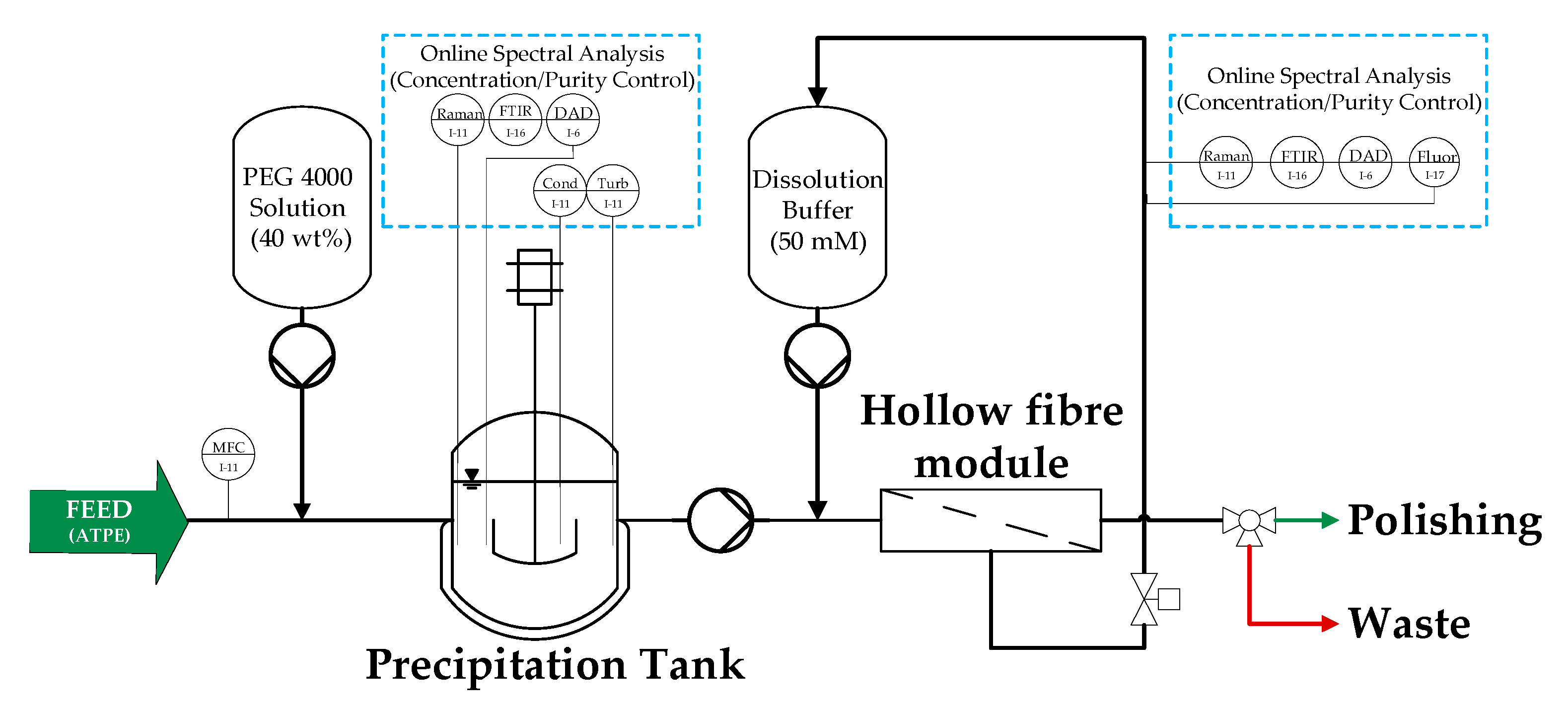
Figure 1 shows a simplified flowsheet of one precipitation subunit, which consist of a stirred tank reactor where precipitation proceeds and a hollow fiber module where filtration and dissolution take place. After precipitation in the tank, precipitates are transferred to the filter module and are deposited onto the membrane through dead-end filtration. Hereby, valves are such positioned, that the permeate is discharged into the waste. Afterwards valves are closed to enable a closed loop for dissolution. Once the online measured redissolution of mAb is sufficient, valves are opened, and the intermediate product is filtered through the membrane and transferred to chromatography. The interconnection of several subunits such as the one shown in Figure 1 enable continuous processing of the incoming feed (light phase, LP) from aqueous-two phase extraction (ATPE).

The aim of this work is, firstly, a feasibility study on spectroscopic methods to monitor mAb concentration, yield, and purity throughout the precipitation process. For this purpose, the compatibility of the individual detectors is tested. Secondly, the combination of several detectors is tested, and a recommendation is given which detector is best suited for the precipitation unit. Thirdly, an advanced process control (APC) concept is proposed, which uses the online measured data for process optimization and monitoring the actual state of the process.

2. Materials and Methods

During this experimental series, three process cycles, starting with cultivation followed by extraction, precipitation, chromatography, and the UF/DF were performed at the Institute of Thermal Process Engineering. This paper only deals with the precipitation part. The overview of the whole study has been previously published [6]. Cell culture broth is obtained through cultivation of Chinese hamster ovary cells (CHO DG44) producing an industrially interesting monoclonal antibody (mAb) from the subclass IgG1. Detailed information about culture broth [1,3,4,5,41] and ATPE [4,51] have also been previously published.

The precipitation unit in this work consist of two parts: the precipitation step, where mAb precipitates from the feed solution and the dissolution, where resolution of these precipitates takes place. Operation procedure is conducted similar to a previous work described by Lohmann et al. [4]. In this work batch units are connected to a continuous process. Precipitation is accomplished after ATPE from the polymer rich phase (light phase, LP) using a Polyethylene glycol (PEG 4000) stock solution (40 wt %, pellets, from Sigma Aldrich, dissolved in 60 wt % HQ H₂O). For complete precipitation, streams are adjusted to result in a PEG content of 12 wt % respective to light phase volume. Precipitation sampling required a workaround because precipitation is such a spontaneous process. In order to train the partial-least-square model (PLS) for spectral analysis several equilibrium stages are used to simulate the precipitation and display the changes in the spectra. Samples from 1 wt % to 17 wt % PEG (in 2 wt % PEG steps) are prepared.

Solid–liquid separation is performed using a hollow fiber module with a pore size of 0.2 µm (88 cm², Midikros, Repligen Corporation, Rancho Dominguez, CA, USA). To minimize product loss, the module is operated in dead end mode to completely deposit the precipitates onto the membrane surface. Precipitates are filtered in dead-end mode at constant flux until the critical transmembrane pressure of 1800 mbar is reached. Thereafter, the feed stream is switched to the next filter module. Afterwards, precipitates are washed with PEG 4000 (12 wt %) solution to maintain precipitation conditions and prevent resolution of mAb. Subsequently, dissolution is performed by recycling a 50 mM sodium dihydrogen phosphate/disodium phosphate buffer at pH = 5.5 along the fibers for 14 h. Sampling rate in dissolution was every 10 mins during first two hours and then one sample every 60 mins. After dissolution, the pH is adjusted to 3.7 and held for 60 min for virus inactivation [52]. Investigation of suitable PAT detectors and sensors (pH, Turbidity, conductivity) is performed separately for precipitation and dissolution. The following PAT detectors have been used throughout the study: Raman (785 nm laser, 1.5 mW, Ocean Insight, Ostfildern, Germany, with an InPhotonics Raman probe), FTIR (Alpha II, Bruker, Billerica, MA, USA), DAD (Smartline DAD 2600, Knauer Wissenschaftliche Geräte GmbH, Berlin, Germany), and fluorescence (Jasco FP-2020 Fluorescence detector). With the exception that the fluorescence detector is not used in precipitation due to precipitates which are harmful for the flow cells of the fluorescence detector and they bias the measurement results. PLS models are built for three analytes: target component (TC), concentration of high molecular weight impurities (HMW) and light weight molecular impurities (LMW), investigating the change of concentration and purity over process time.

2.1. Analytics

2.1.1. Online

Data acquisition in Raman spectroscopy is set to automatically average a total of three spectra, with an integration time of 1s each. Data acquisition in FTIR spectroscopy is set to automatically average a total of 60 spectra, with an integration time of 1s each. Data acquisition in UV-Vis spectroscopy is set to continuously record at a sampling rate of 0.2 s, each of which have 32 msec of integration time. Data acquisition in fluorescence spectroscopy (Jasco FP-2020 Fluorescence detector) is conducted with a gain factor of 1. Spectra are measured with an excitation wavelength of 280 nm and the emission spectra is detected between 280 and 900 nm. For each sample at least three spectra are measured and averaged prior to PLS-regression.

2.1.2. Offline

The monoclonal antibody is quantified by Protein A chromatography (PA ID Sensor Cartridge, Applied Biosystems, Bedford, MA, USA). Dulbecco’s PBS buffer (Sigma-Aldrich, St. Louis, MO, USA) is used as loading buffer at pH of 7.4 and as elution buffer at pH of 2.6. The size exclusion chromatography (SEC) is performed with a YarraTM 3µm SEC 3000 column (Phenomenex Ltd., Aschaffenburg, Germany) utilizing 0.1 M Na₂SO₄, 0.1 M Na₂HPO₄, and 0.1 M NaH₂PO₄ (Merck KGaA, Darmstadt, Germany) as buffering system. The absorbance for both methods is monitored at 280 nm.

2.2. Preprocessing of Spectral Data

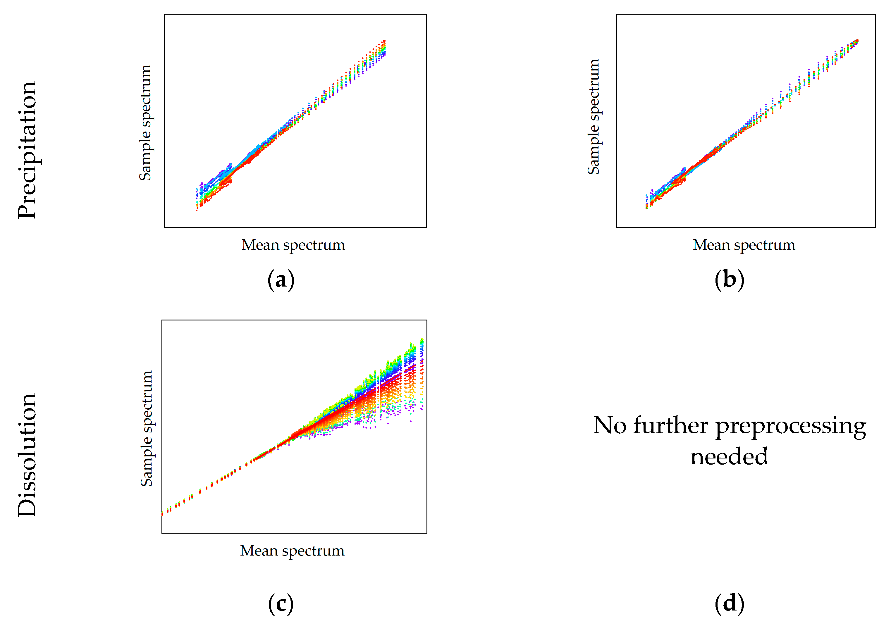
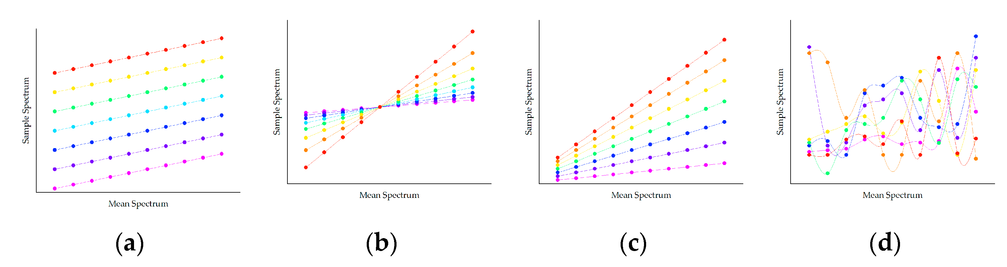
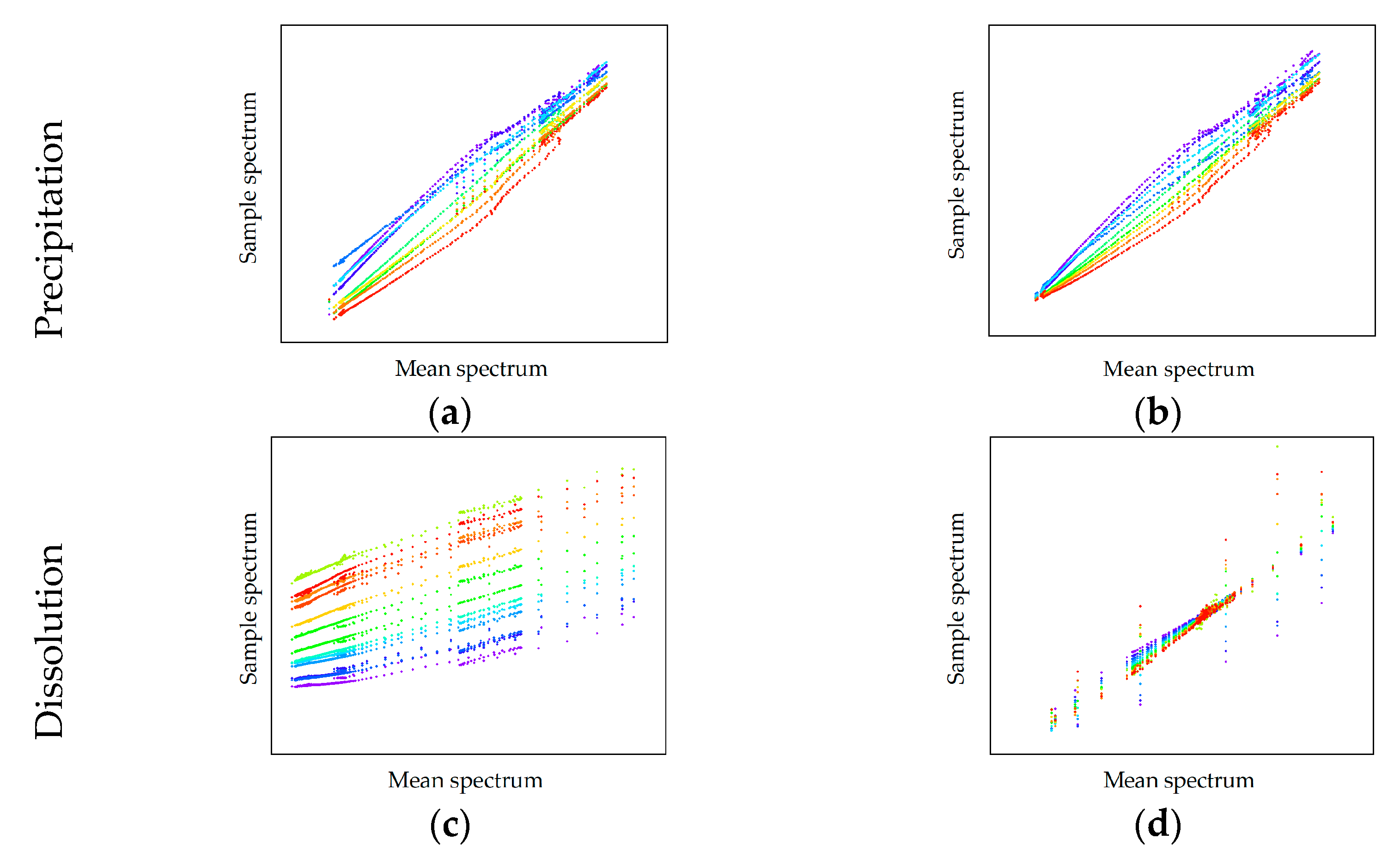
Spectral data are processed and analyzed using Unscrambler^® X (Camo Analytics AS, Oslo, Norway). First, raw spectral data are trimmed to the fingerprint region for proteins which is for Raman 1800–400 cm⁻¹ and for FTIR 1800–900 cm⁻¹ respectively. DAD and Fluorescence spectra are not trimmed and used completely for analysis. The preprocessing strategy can vary for the obtained data and must be adjusted. To perform an adapted preprocessing, descriptive statistic is analyzed. Hereby, the scatter effects plot is used, which depicts the sample spectrum against the mean spectrum. The following scatter effects shown in Figure 2 can be present: (a) additive effects, (b) scatter effects, (c) additive and scatter effects and (d) complex effects.

Additive effects are eliminated by conducting a derivation or applying a baseline correction. Multiplicative scatter effects can be removed using the method of standard normal variate (SNV) or a multiplicative scatter correction (MSC). Combinations of additive and multiplicative effects are removed by a combination of baseline correction, and scatter correction and complex effects can be eliminated by using an extended multiplicative scatter correction (EMSC). Depending on the scatter effects, the pre-processing is adapted to extract a maximal information content. Pre-processed spectra are then used to correlate the changes in component concentration to the changes in spectral intensity at specific spectral regions by partial least squares regression. A maximum of four principal components was allowed in the regression to not overfit the data. The quality of the model was evaluated by means of spectral line loadings plot, score plot, and the plot of explained variance against number of principal components. If Pat inline would be feasible, another tool for APC would be a suitable digital twin based on process modeling as described in the following. 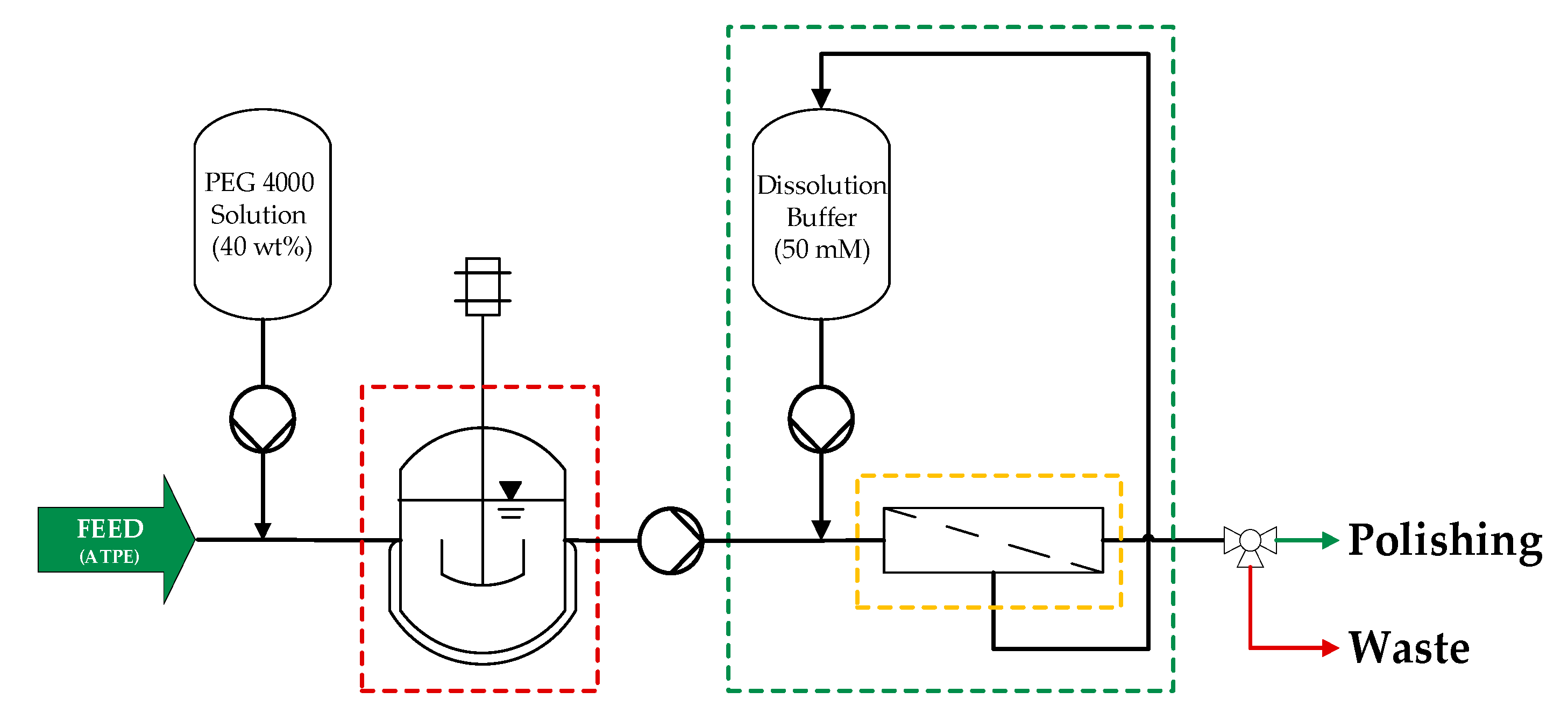Based on the precipitation unit proposed in a previous work [4], the process model for the APC concept is presented. The model is divided in to three sub models: Precipitation of mAb, filtration of precipitates and resolution of precipitated mAb which is schematically shown in Figure 3. Division into sub models is necessary for separation of effects within precipitation, filtration, and dissolution.

2.3. Precipitation Model

Precipitation takes place batchwise and is modeled as a continuous stirred tank reactor (CSTR). Precipitation with PEG is a spontaneous process. In literature fractal analysis is used to infer the rate limiting step in precipitation. Hereby, the fractal dimension is used to categorize in reaction limited and diffusion limited precipitation. Accordingly, a reaction-limited precipitation is present at low fractal dimensions of 1.7 and a diffusion-limited one at a fractal dimension of 2.4 [53,54]. Satzer et al. have demonstrated a methodology to 3D reconstruct precipitates using light microscopy in combination with advanced image evaluation [55]. The 3D reconstructs have been used to perform a fractal analysis to determine fractal dimension and fractality on micro- and nanoscale. Satzer et al. showed that PEG precipitates have an average fractal dimension of 2.4 [55].

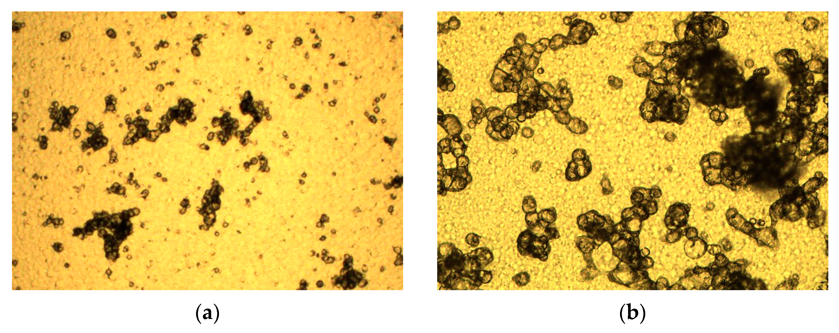
To evaluate this, precipitates have been analyzed through light microscopy, which has shown that the particles consist of sphere-like structures that agglomerate and tend to monofractility (see Figure 4). Fractality is determined through the method published by Satzer et al. [55] and lead to comparable results of a fractality of 2.4. Therefore, it is expected to be a diffusion-limited precipitation, which is in good agreement with the experimental results described in Lohmann et al. [4] and the theory that IgG diffuses very slowly due to its size.

For this reason, concentration decrease during precipitation is described as a reactive crystallization due to the spontaneous and diffusion-limited process. The concentration change in the supernatant is calculated by applying a 1st order reaction kinetics [56] as can be seen in Equation (1):

$$r_{prec}=-k_{prec}*\left(c_{mAb}-c_{eq}\right)$$

(1)

where $r_{prec}$ represents the reaction rate which is associated with the concentration change of the target component over process time, $k_{prec}$ the rate constant of precipitation, $c_{mAb}$ the instantaneous mAb concentration and $c_{e{q}_{prec}}$ its equilibrium concentration. The precipitation constant was determined via turbidity in a previous work [4]. In literature precipitation is described as the change of chemical potential which leads to formation of dense precipitates as their status is more stable under new surrounding conditions [57]. This results in a shift of protein solubility (S) which is described by Equation (2) [58]. In the proposed model the maximal protein solubility equals the equilibrium concentration of mAb ($c_{eq}$).

$$\log \left(S\right)=-\beta *\omega +\kappa$$

(2)

Whereas, $\beta$ stands for precipitation efficiency, $\omega$ for the weight percentage of PEG added to light phase and $\kappa$ the intrinsic protein solubility [58]. Sim et al. derived a model to describe the precipitation efficiency in presence of PEG molecules based on attractive depletion and excluded volume [57,59]. $\beta$ is determined as described in Sim et al. [57] Values for $\gamma = 0.076$ and $\delta =-0.045$ are also adopted from [57]. The needed weight percentage of PEG for complete precipitation is determined through equilibrium experiments in a previous work [4].

$$\beta =\gamma *r_{h,PEG}^{0.211}*r_{h,Protein}+\delta *r_{h,Protein}$$

(3)

Hydrodynamic radius for the target component is calculated with Equation (4). The hydrodynamic radius for PEG is obtained from literature [59].

$$r_{h,Protein }={\left(\frac{3\eta M_{r,Protein}}{4\pi 2.5 N_A }\right)}^{\frac{1}{3}}$$

(4)

2.4. Filtration Model

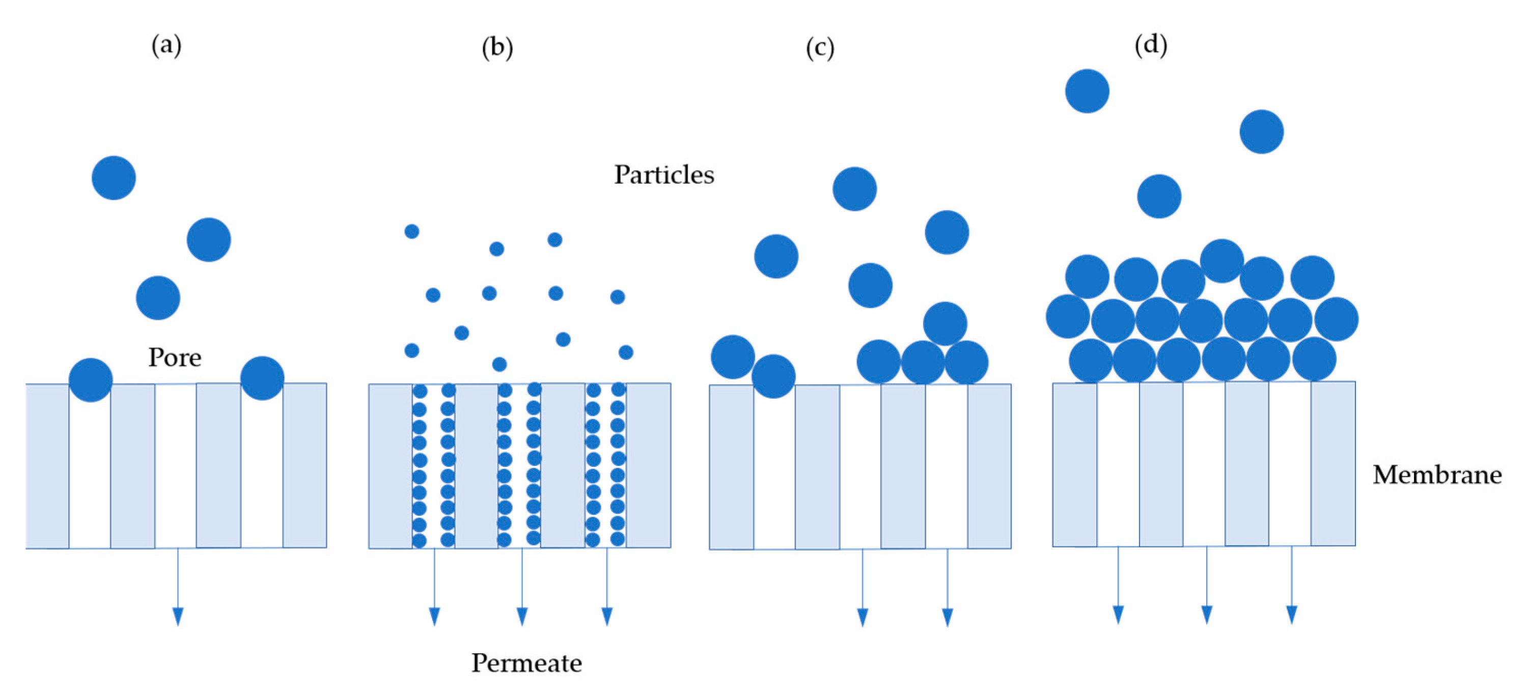
The filtration of precipitates is performed with a hollow fiber module through dead-end filtration at constant flux. Hollow fiber filters are not designed for dead end operation, but their design has an advantage for subsequent redissolution. Modeling of dead-end filtration is commonly described as the occurring blocking mechanism, which can be calculated as a pressure change over time [60,61,62]. The commonly used blocking mechanisms are depicted in Figure 5 [62]. Complete blocking occurs when the particles to be filtered have approximately the same size as the pores in the membrane (Figure 5a). Standard blocking appears while particles are smaller than the pores and deposit inside the pores (Figure 5b). Cake filtration occurs when the particles form a dense layer on the membrane (Figure 5d) and intermediate blocking is a composed blocking mechanism of cake filtration and complete blocking (Figure 5c). A widely maintained opinion in literature is that description by only one blocking mechanism is not sufficient due to several superimposed effects [62,63,64,65].

In this case the filtration could be described best by a composite model of cake filtration (see Equation (5)) and standard blocking (see Equation (6)). First, cake filtration occurs which changes to standard blocking. $p_{0,cake}$ is the initial pressure at the beginning of the experiment and $p_{0,standard}$ means the current pressure at the switching point to standard blocking. $J_0$ is the transmembrane flux, which is kept constant throughout filtration and $v$ stands for the membrane specific volume. Blocking constants $K_s$ and $K_c$ are determined for the specific filter with a calibration experiment in advance.

$$p=\left(1+K_c·J_0·v\right)·p_{0,cake}$$

(5)

$$p=\frac{p_{0,standard}}{{\left(1-\left(K_s·\frac{v}{2}\right)\right)}^2}$$

(6)

2.5. Dissolution Model

Model equations for dissolution are based on the same mechanism as precipitation, however, with a different mass transfer coefficient for dissolution. Product losses in dissolution may occur due to two cases: limitation through the feed concentration or the maximal protein solubility. The limitation by the feed concentration ($c_{max}$) appears when the equilibrium concentration in the dissolution buffer is significantly higher than the mAb concentration in the feed. In this case the complete initially precipitated mass of mAb can be redissolved (see Equation (7)). If the depletion of the PEG or the volume ratio (DR) between feed and buffer is too low, limitation by equilibrium concentration (see Equation (8)) is the result due to a residual PEG content which should not exceed 3 wt % [13]. $r_{diss}$ describes the reaction kinetic dissolution of precipitates dependent on the circulation flowrate through the fibers. $c_{mAb}$ it the current mAb concentration dissolved in the dissolution buffer and $c_{e{q}_{diss}}$ the equilibrium concentration of mAb in dissolution. As described before, equilibrium parameters do not change in dissolution, but the equilibrium concentration does due to reduction of the PEG content in solution. DR describes the ratio between feed and dissolution buffer volume.

$$r_{diss}= k_{diss}·\left(c_{e{q}_{diss}}-c_{mAb}\right)$$

(7)

The mass transfer from the membrane surface back into dissolution is dependent on the recirculation flow rate trough the fibers and is calculated as reversed concentration polarization. Material transfer in concentration polarization is described through the coefficient $k_{eff}$ which is dependent on the flow regime. First, Reynolds number (Re) must be calculated for identification of the current flow regime. This relates inertial forces and viscous forces in the fluid [66].

$$Re=u_{eff}·\frac{\rho }{\eta }$$

(8)

The effective velocity is referring to the empty tube velocity. $\dot{V}$ is the flow rate through one fiber during dissolution, A the cross-sectional area of all fibers and $ϵ$ the porosity.

$$u_{eff}=\frac{\dot{V}}{A·ϵ}$$

(9)

Second, Schmid number Sc is determined for relation of diffusive impulse transport to diffusive mass transport. Whereas, D stands for diffusion coefficient of mAb, $\eta$ the viscosity of the fluid and $\rho$ for the density [67].

$$Sc=\frac{\eta }{\rho ·D}$$

(10)

From Reynolds and Schmidt follows the Sherwood number which describes the ratio of the effective amount of substance transferred to the amount of substance transported by diffusion. The correlation by Leveque applies only for Reynolds number below 1800 [68]:

$$Sh=1.62·R{e}^{0.33}·S{c}^{0.33}·{\left(\frac{d_H}{L_{ch}}\right)}^{0.33} \mathrm{Re}<1800$$

(11)

With d_H as hydraulic diameter and L_ch as characteristic length of the module. Using the Sherwood number, the effective mass transfer coefficient related to the surface of the membrane follows as:

$$k_{eff}=Sh·\frac{D}{d_H}$$

(12)

The time dependent parameter $k_{diss}$ of the process model is obtained by multiplication of $k_{eff}$ with the volume specific surface of the fibers.

$$k_{diss}=a·k_{eff}$$

(13)

3. PAT Feasibility Study Results and Discussion

Due to the different experimental setup, the results for precipitation and dissolution are shown separately. Investigated components are high molecular weight impurities (HMWs), Target component (TC) and low molecular weight impurities (LMWs). Categorization of very good (1 < R² < 0.9), moderate (0.9 < R² < 0.8) and poor (R² < 0.8) is based on the R² of generated PLS models. These ranges are narrow due to the goal to replace standard offline analytics (HCPLs).

3.1. Raman Spectroscopy

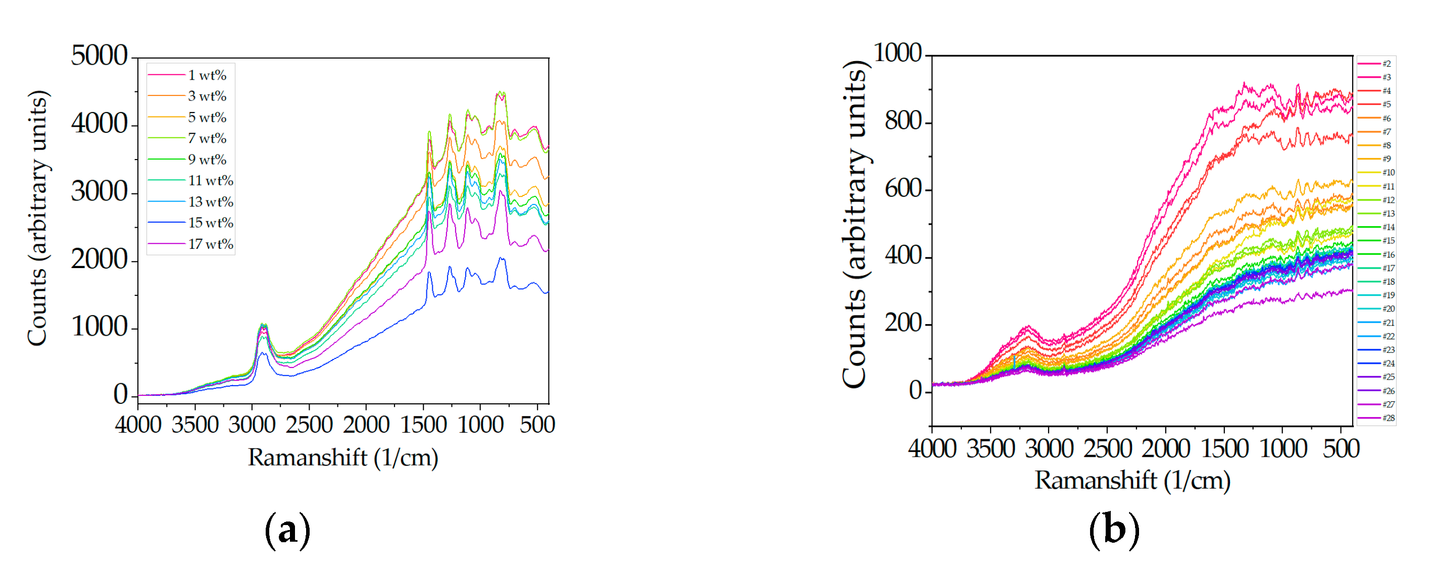
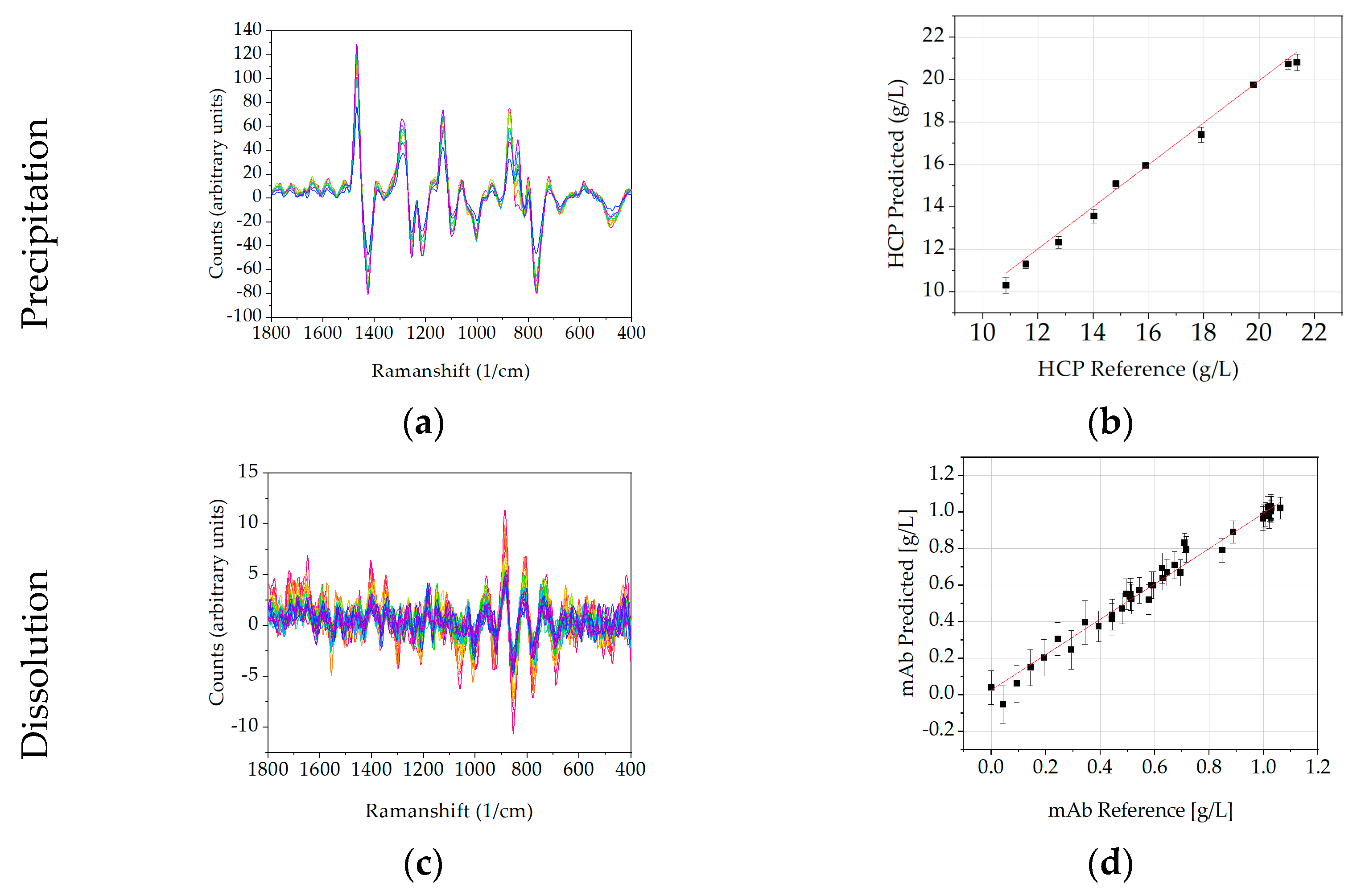
In this section Raman spectral data are discussed, first for precipitation and following for dissolution. The results (mAb titer and purity) obtained in dissolution are the results of interest for the following unit operation. First, raw data are reduced to 1800–400 cm⁻¹ Raman shift equally for precipitation and dissolution results. It becomes obvious, that spectral raw data for both steps are very distinct (Figure 6a,b). This can be explained by the different matrix of the samples. In precipitation the continuous phase is still the light phase obtained from ATPE, including the phase forming components phosphate and PEG 400 as well as the majority of impurities generated during USP.

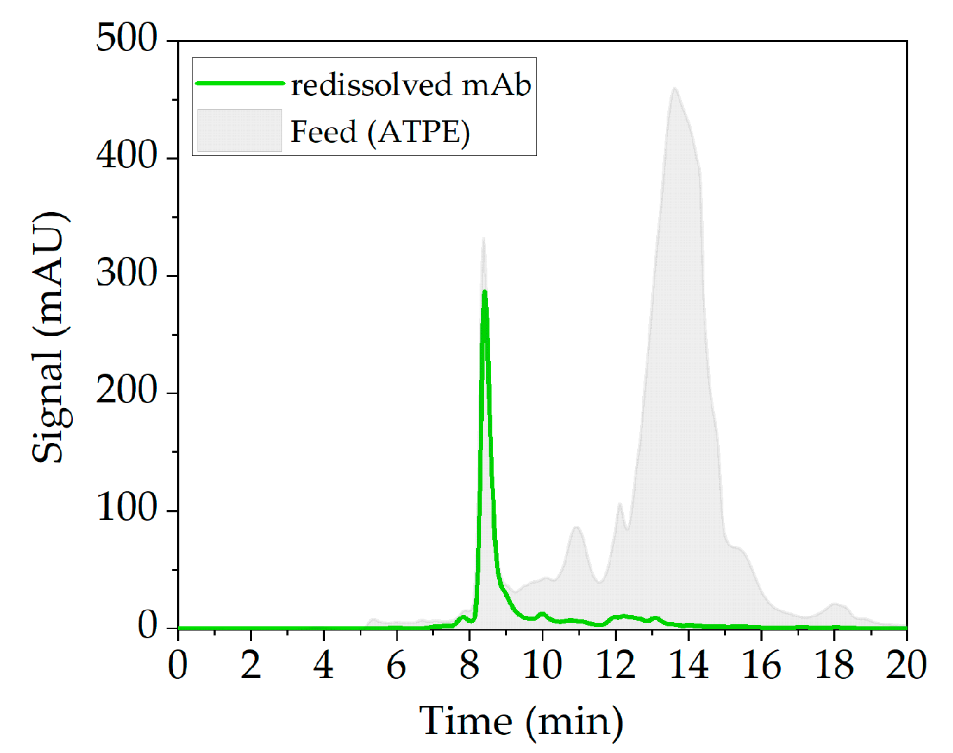
The purity of light phase is usually between $15\pm 2\%$ and can be improved to $85 \pm 5\%$ through precipitation and the subsequent filtration. Further, the surrounding medium is exchanged in dissolution with a sodium phosphate buffer. Figure 7 shows a SEC chromatogram to visualize the purity improvement gained through the precipitation unit. Hence, the described operation procedure does not only result in a significant gain in purity but also in the strong visible differences of the spectroscopic data between precipitation and dissolution in Figure 6.

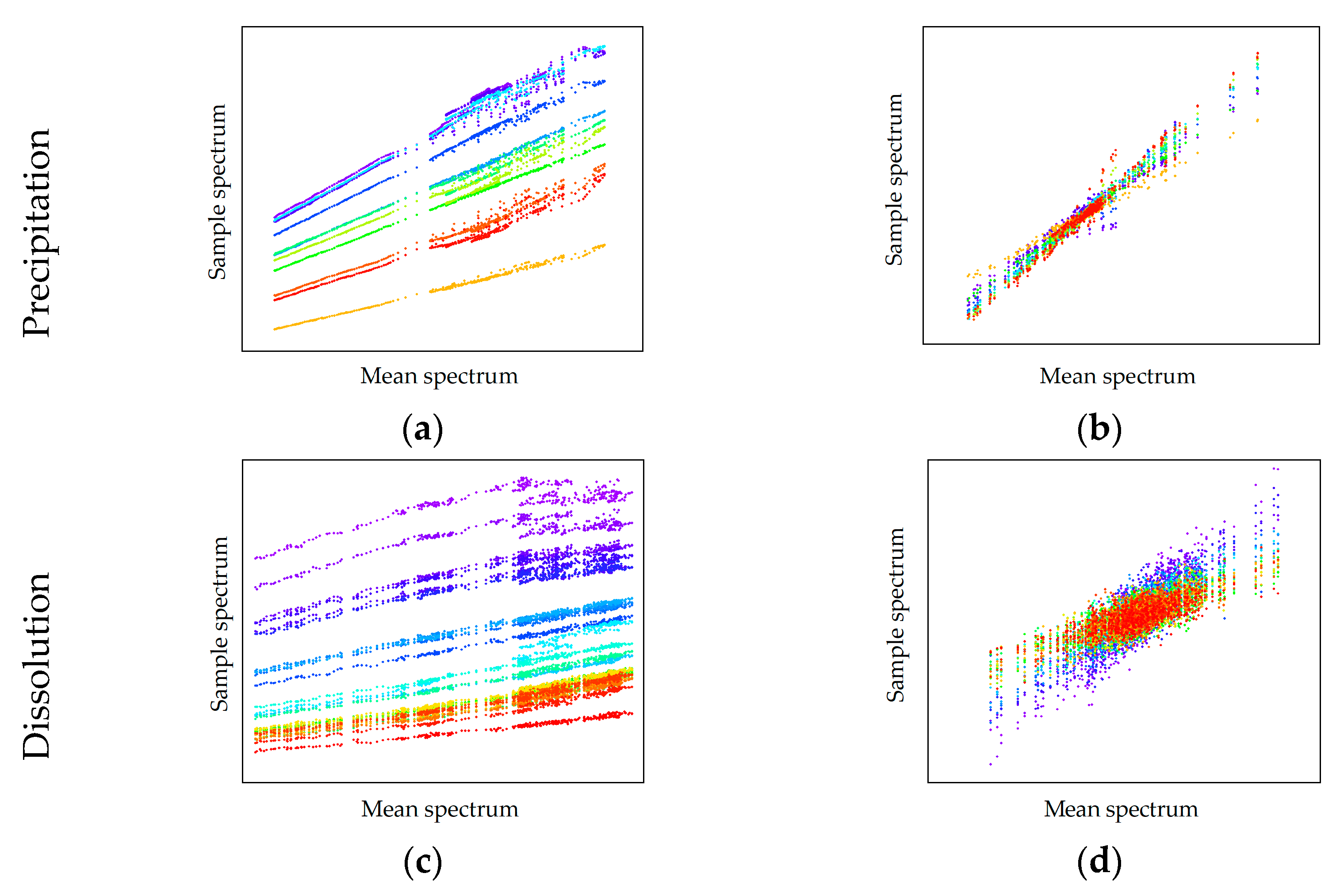
Preprocessing is conducted due to evaluation of the scatter effects plots, which are depicted in Figure 8a for precipitation and in Figure 8c for dissolution. Parallel and superimposed scatter effects represent a linear offset in spectral raw data and are reduced with a first derivation using Savitzky Golay with three smoothing points. New scatter effects seem to run through one point with varying slopes and are depicted in Figure 8b,d. Therefore, SNV and MSC are tested. Neither SNV nor MSC gave satisfying result. Hence, data were not preprocessed any further.

In the case of Raman, preprocessing was equal for precipitation and dissolution. The preprocessed spectral data are presented in Figure 9a,c. PLS regression for precipitation was very good (R² of 0.95) referring to LMWs for HMWs (R² of 0.62) and the Target (R² of 0.63) component only poor correlations are found. In dissolution convincing results are achieved for the target component (R² of 0.93) only. Correlation for LMWs and HMWs could not be found.

Prediction of purity in precipitation and dissolution is very poor for LMWs (R² of 0.46 and R² of 0.22) and HMWs (R² of 0.3 and R² of 0.13). However, the purity prediction for the target component resulted in R² of 0.66 for precipitation and R² of 0.85 for dissolution which is acceptable. It can be concluded that Raman is a suitable detector in precipitation for LMWs and in dissolution for the target component.

3.2. Fourier-Transform Infrared Spectroscopy

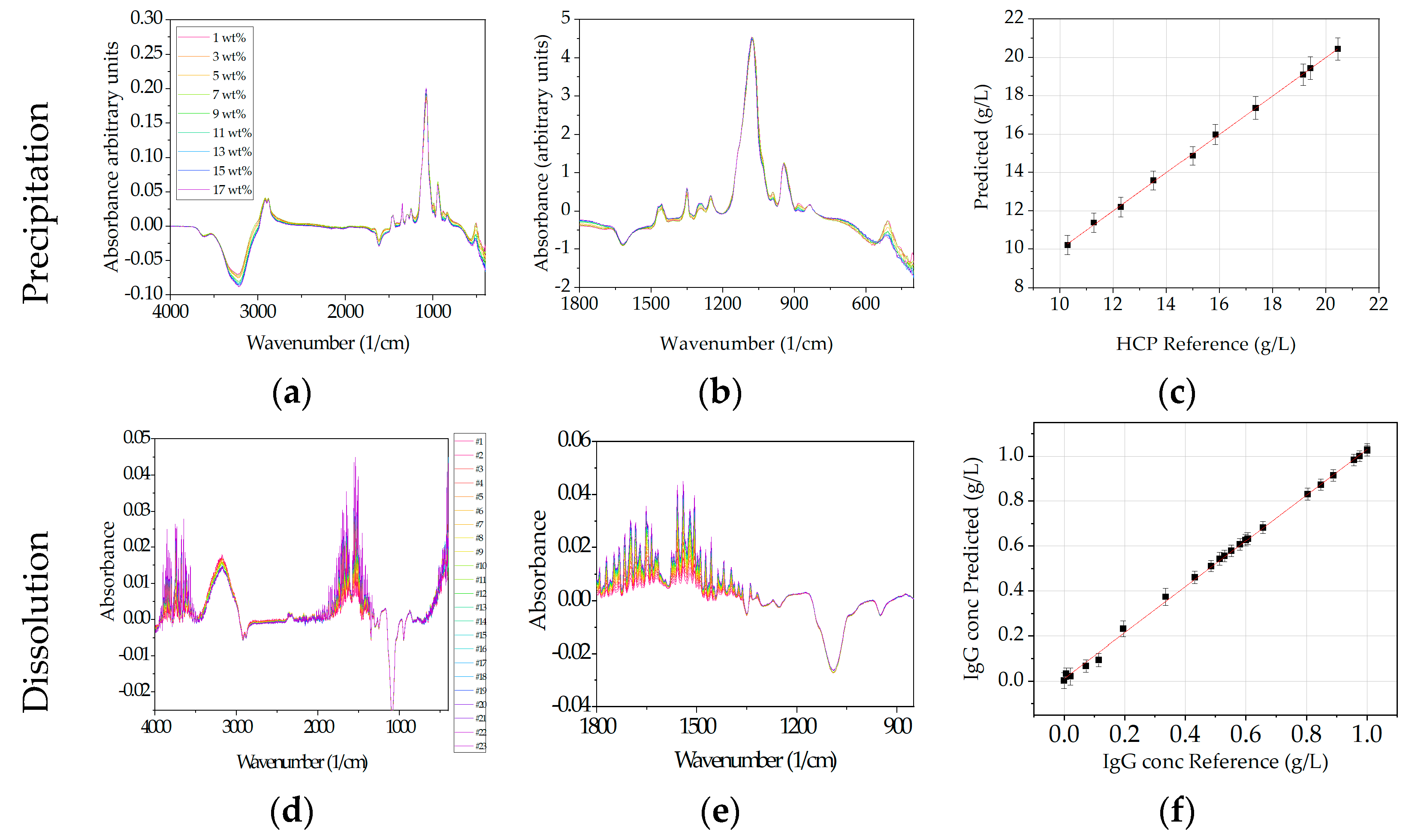
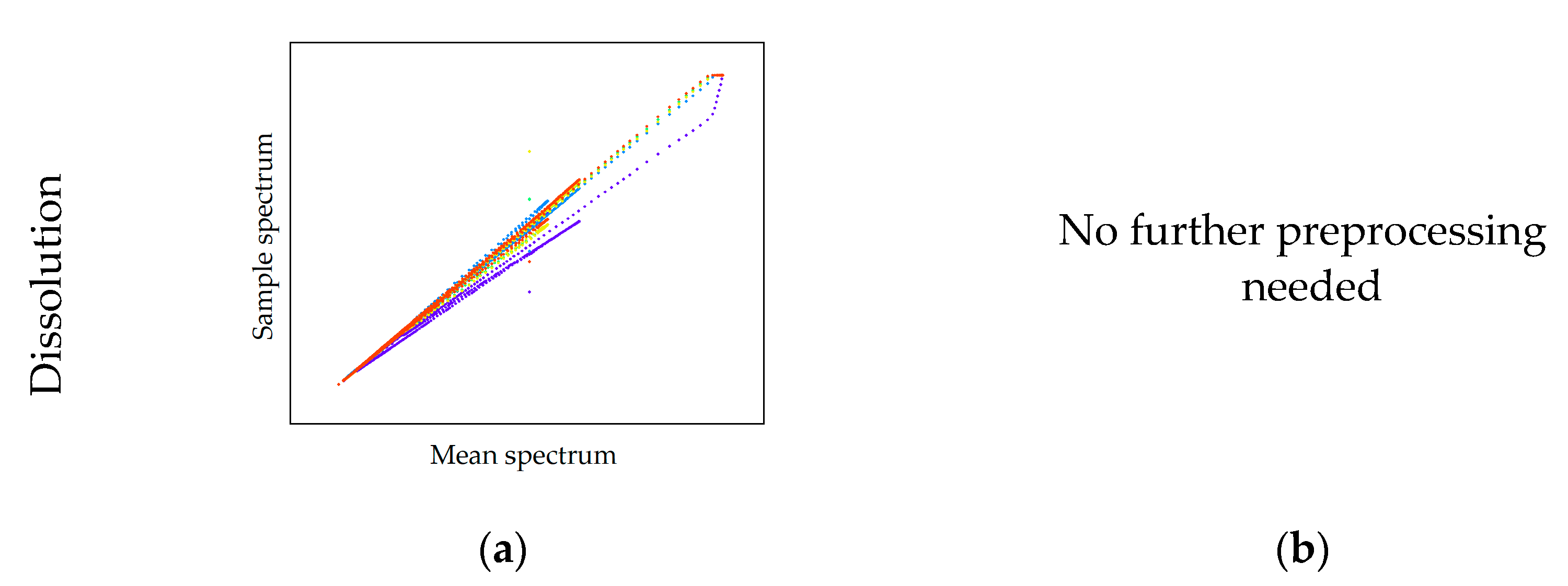
The evaluation of the spectral data for the FTIR is carried out in accordance with the procedure in the previous Section 3.1 FTIR spectral raw data are also reduced to 1800–400 cm⁻¹ wavenumber equally for precipitation and dissolution. Analyzing spectral raw data during precipitation, only slight differences are observed which is mainly the magnitude of absorbance. Further preprocessing is performed after evaluation of scatter effects shown Figure 10a,b. Evaluation of scatter effects for precipitation indicate that scatter effects run through one point with different slopes, wherefore, SNV using Savitzky Golay with three smoothing points is chosen as pretreatment. The new scatter effects plot changed slightly which indicates that the analyzed data does not contain a lot of overlaying interferences. In contrast, for dissolution larger deviations can be monitored between wavenumbers 1800–1400 cm⁻¹. Scatter effects for dissolution do not show one of the effects mentioned above, wherefore, no further preprocessing is necessary in case of FTIR data in dissolution.

As an additional analyzation method, a PCA is performed for dissolution raw data, which indicates that most spectral information is located between 1800–850 cm⁻¹. Therefore, spectral data are reduced further to this region (Figure 11b,e). Here again the observation is made, that in precipitation the PLS regression for LMWs is very good with a R² of 0.94 but is very poor for HMWs (R² of 0.43) and the target component (R² of 0.42). In dissolution convincing results are achieved (R² of 0.91) for the target component and only poor results for HMWs (R² of 0.31) and LMWs (R² of 0.54). PLS regression for purity did not lead to any satisfactory results in neither precipitation nor dissolution. Nevertheless, it can be concluded that FTIR is a suitable detector for LMWs during precipitation and for the target component in dissolution.

3.3. Diode-Array Detector

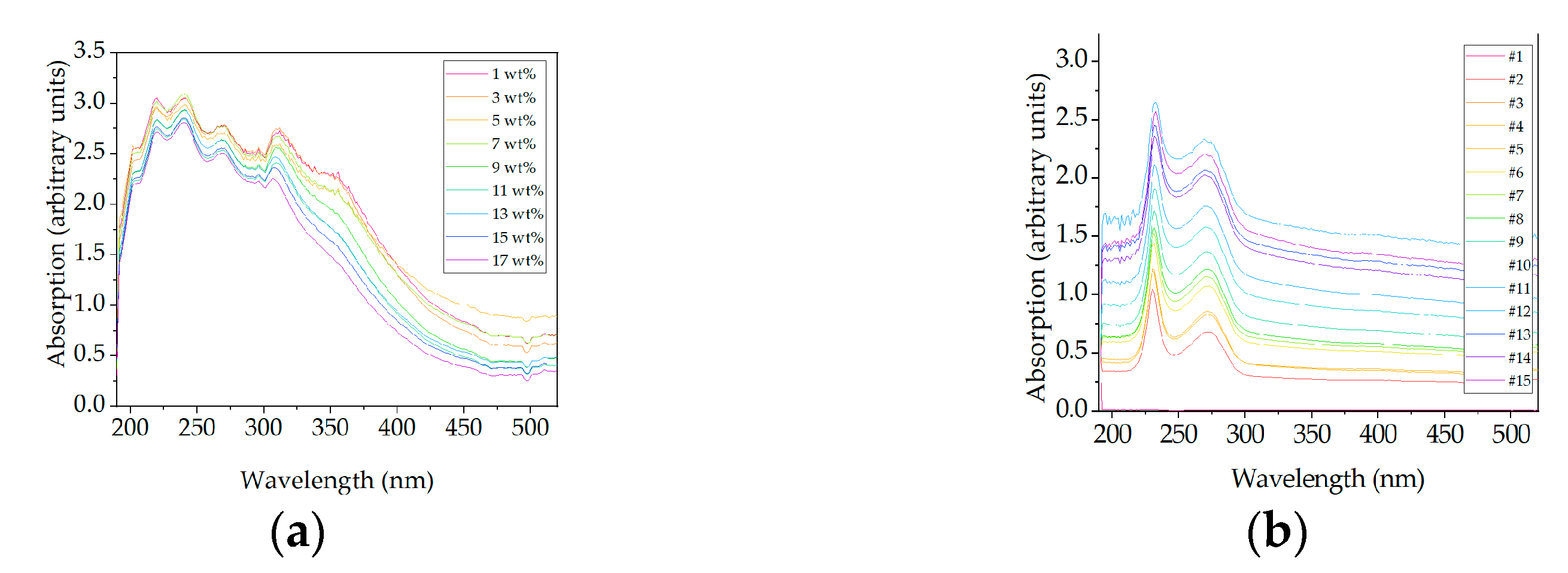
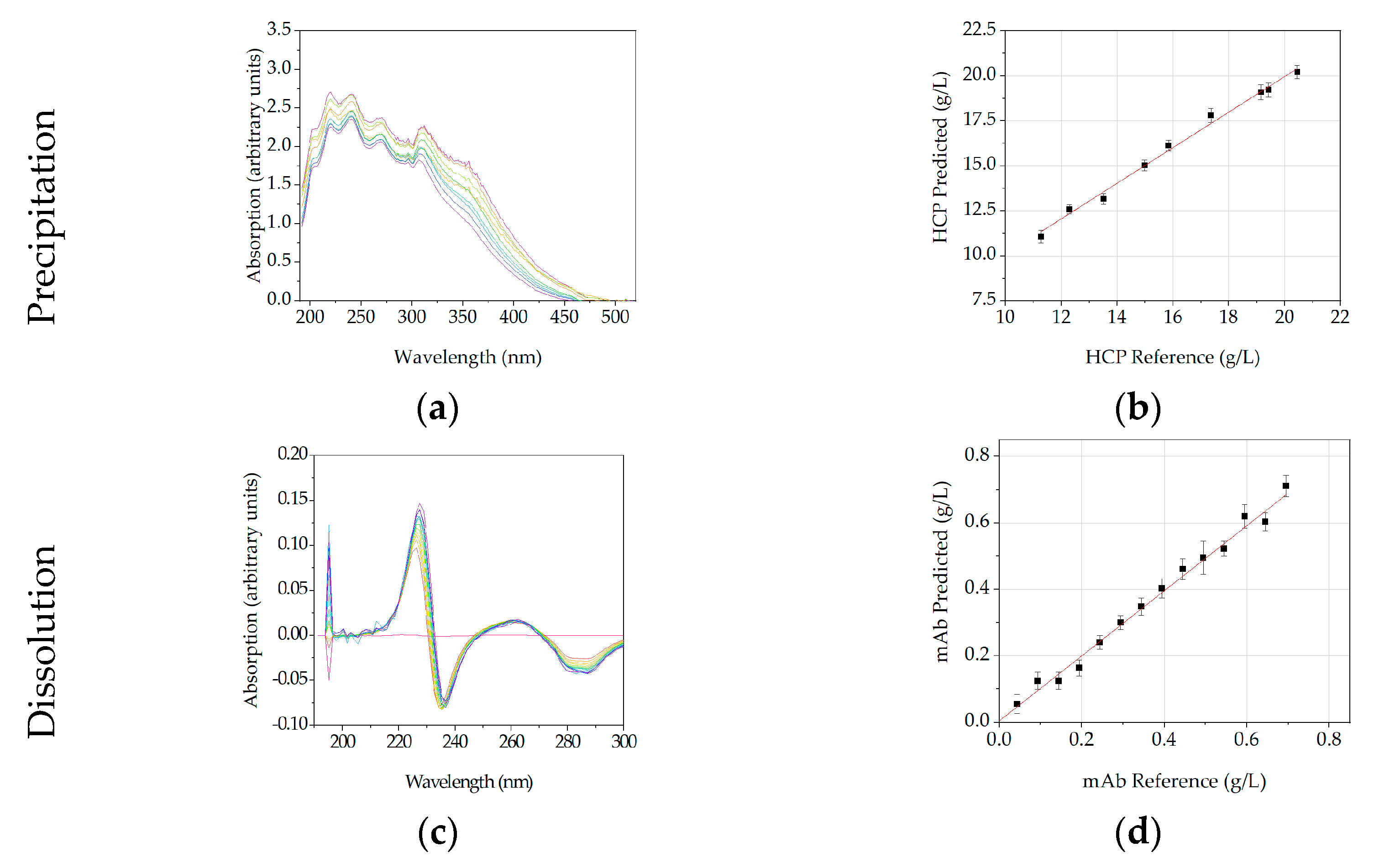
Spectral data of DAD are not reduced and the full spectrum is evaluated ranging from 190 nm to 520 nm. Analyzing spectral raw data for precipitation, arbitrary units decrease for a rising PEG content. This is convincing since less proteins are in solution with an increased PEG amount. A DAD detector can detect proteins reliably, but distinction between different proteins is difficult since most proteins have the highest absorbance at 280 nm. A similar trend can be observed in DAD raw data for dissolution (Figure 12b) but in the opposite direction. Arbitrary units increase steadily with increasing process time, as does the concentration of the re-dissolved antibody. This is to be expected as the absorbance of a DAD increases according to the law of Lambert–Beer.

Evaluation of scatter effects (see Figure 13) lead to a baseline correction in case of precipitation and to a first deviation in case of dissolution (Savitzky Golay with three smoothing points). The DAD results (see Figure 14) fit the previously described observations for FTIR and Raman quite well. The concentration of side components such as LMWs (R² of 0.97) can be described appropriately during precipitation while spectral data in dissolution are suitable for the prediction of the target component (R² of 0.93). Additionally, here the prediction of purity is not satisfactory with R² of 0.57 for LMWs and R² of 0.59 for TC during precipitation.

It can be concluded that DAD is a suitable detector to monitor LMWs in the precipitation process. Furthermore, DAD is appropriate to display the redissolution of the target component. Reliable determination of purity was not possible.

3.4. Fluorescence Detector

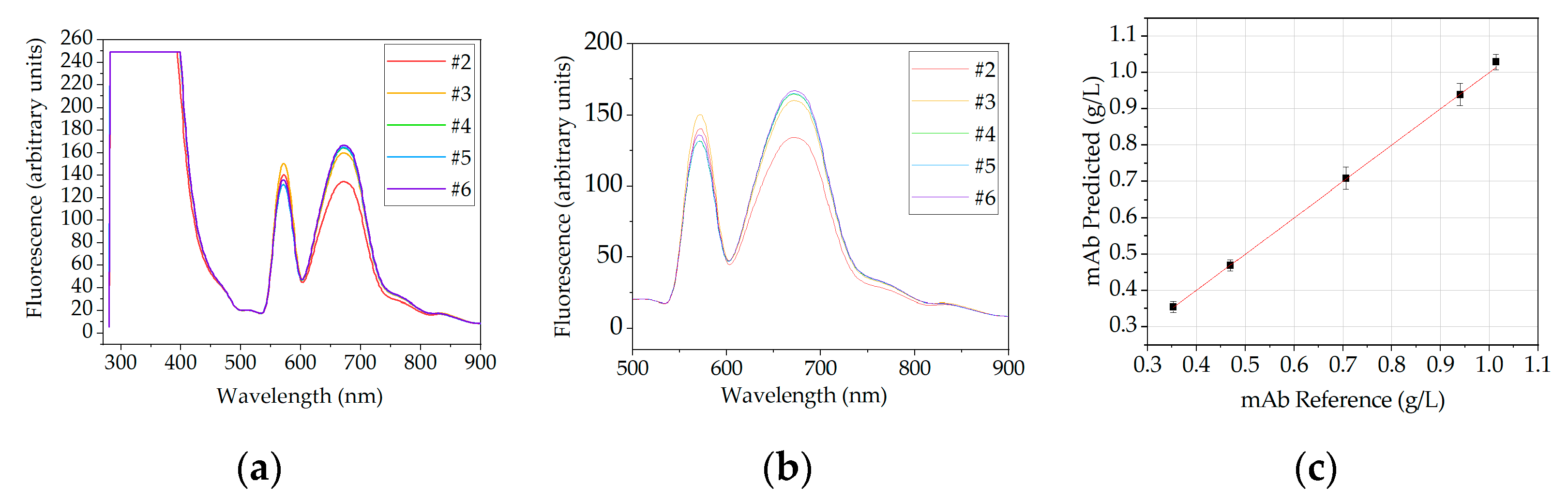
Fluorescence spectra are taken for dissolution only since the precipitates are harmful for the flow cell of the detector. In case of dissolution the entire spectrum ranging from 280 nm to 900 nm is used for analysis. Analyzing the raw data in Figure 15a a fluorescence maximum between 570 and 675 nm can be identified, which describes the concentration increase during dissolution adequately. At the beginning of the dissolution process, the antibody dissolves more rapidly and approaches an equilibrium value over process time. This can also be seen in the arbitrary units of the fluorescence; whose values change proportionally with the increase in concentration measured offline.

Evaluation of scatter effects, which are shown in Figure 16 does not show one of the effects described in Figure 2, hence, no preprocessing of spectral data is performed. The data are just trimmed to 500–900 nm, which is the region of interest. PLS regression resulted in a R² of 0.90 for the concentration increase of the antibody. Purity could not be correlated to the spectral data. The regression results of the concentration prediction is depicted in Figure 15c.

3.5. Combination of Detectors

The combination of several detectors can lead to prediction accuracy and a higher robustness of the process. For this reason, the prediction quality of a combined PLS, which is trained with data from different measurement methods, is tested. Since the concentration and purity during dissolution are decisive for the next unit, only a combination for dissolution is shown. DAD and Raman have each given the best performance, which are summarized in

Table 1. PLS results of process analytical technology (PAT) feasibility study for Raman and DAD referring to mAb concentration and purity.

	Concentration	Purity
Raman	0.93 ± 3.9%	0.85 ± 4.9%
DAD	0.93 ± 2.8%	0.59 ± 2.6%
Combination	0.90 ± 3.9%	0.72 ± 4.9%

for both detectors.

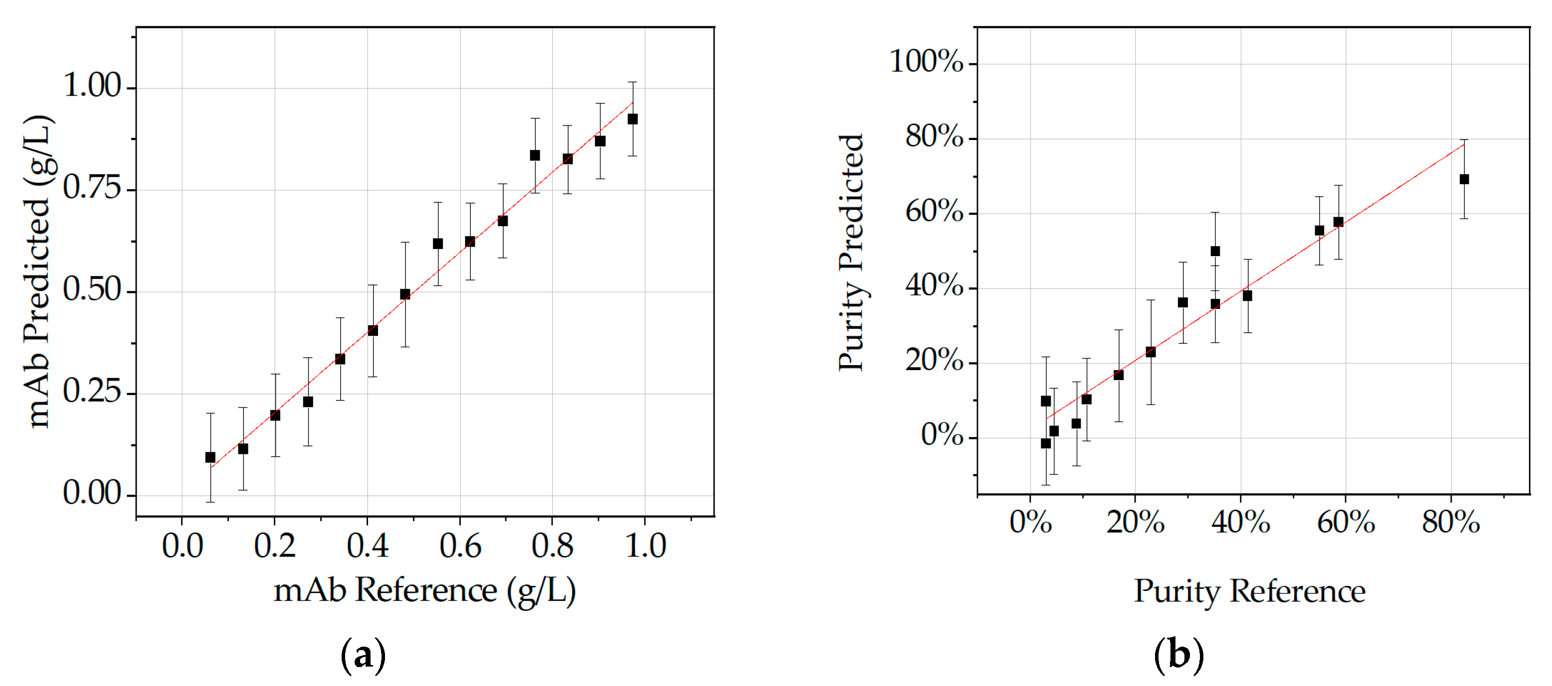
Regression results of the generated PLS model can be seen in Figure 17a shows the regression results for the concentration of the target component and (b) results for the purity prediction. Both detectors in combination achieved a R² of 0.90 for concentration and a R² of 0.72 for purity. This is slightly worse than the results for the detectors alone, but still provides a satisfactory prediction for target component and the purity. Moreover, prediction of purity with a DAD alone is not sufficient. The quality of the data gains in any case because Raman and DAD are based on two different measurement methods and the combination of two orthogonal detectors improves the robustness of online analysis method.

3.6. Additional Process Data of Sensors

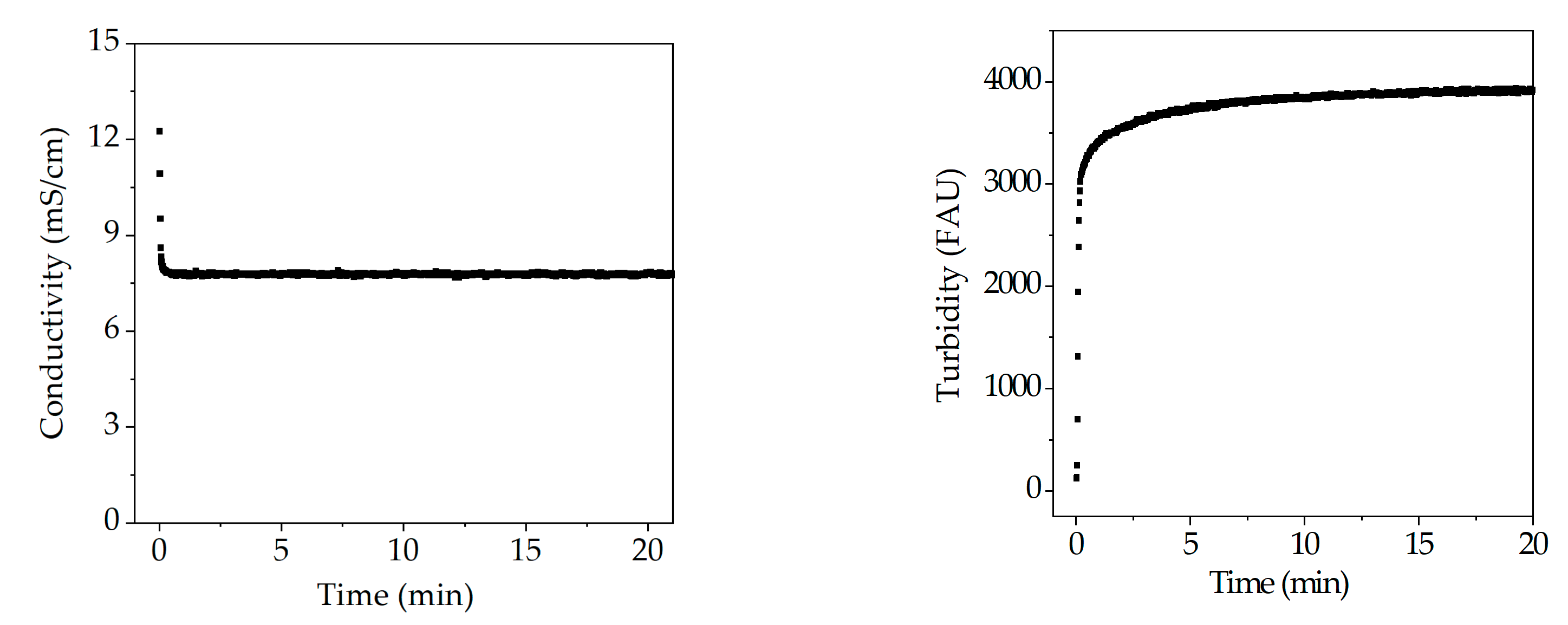
In this section further detectors are evaluated within the PAT concept. Sensors can be used to monitor changes during the manufacturing process. Investigation of pH, conductivity and turbidity sensors during precipitation are shown in Figure 18. pH value remains constant throughout precipitation which indicates that no process information can be correlated to this metrology. Light phase has a conductivity of approximately 12 mS/cm in contrast to the PEG solution, which is not conductive. Therefore, conductivity drops as soon as PEG is added and remains constant afterwards. Conductivity indicates the composition of the dispersion. Hence, conductivity can be used to monitor the component ratio between light phase and PEG 4000 online within a PAT concept to ensure optimal precipitation conditions. Turbidity has, as conductivity, a strong deflection during addition of PEG, because precipitate formation occurs instantaneous. For this reason, turbidity is a measure for the precipitation progress. However, turbidity is not specific to one component, but it gives an estimate on process duration.

Utilization of the different sensors during the dissolution step did not lead to any results. The pH value remained constant due to the buffering system, consisting of sodium dihydrogen phosphate and disodium phosphate. Overall conductivity in the system also corresponded to the conductivity of the dissolution buffer. Turbidity also gave no result, which is not surprising, since precipitates go back into solution. According to this study, Raman is recommended as a detector for precipitation, since it has shown good results in the precipitation and the subsequent dissolution with respect to the target component but also side components (LMWs). Additionally, the purity of the target component in the dissolution could be correlated. As an orthogonal measurement strategy, a DAD is recommended. Furthermore, a conductivity probe is recommended as PAT control strategy for detection of optimal precipitation conditions.

4. APC Proposal and Simulation Studies

Variations in product titer and purity of the target component are to be expected in bioprocesses. These may occur, e.g., due to a reduced growth rate of cells or through limitation/inhibition by the substrate. The reasons for titer and purity fluctuations are divers. The question is whether the precipitation unit presented can react to such fluctuations. Further, how online measurement techniques can be integrated to monitor the actual conditions present in the process. The digital twin is fed with the input data after ATPE and the online measured spectral data. The model estimates new process parameters and generates control values to ensure compliance of the critical quality attributes.

In this section an overview of process procedure of the precipitation unit is given as well as a simulation study on reaction possibilities to process deviation. Furthermore, the benefits of the proposed APC are presented.

4.1. Operation of Precipitation Unit

To begin with this section on APC and simulation studies, the function of the precipitation unit is explained for a better process comprehension. Basically, the precipitation unit consists of four subunits which has been defined in Figure 1. In the continuous set up, the individual precipitation tanks of the subunits are merged into one tank. In the following the operation of the continuous unit is explained. Throughout the process each subunit passes through different phases in a certain order, namely filtration of precipitates, followed by redissolution and, finally, a rinsing process to regenerate the membrane. Further, each subunit passes all phases multiple times, but with a time delay to ensure continuous processing of the incoming feed (light phase from ATPE) and to provide a constant output stream. 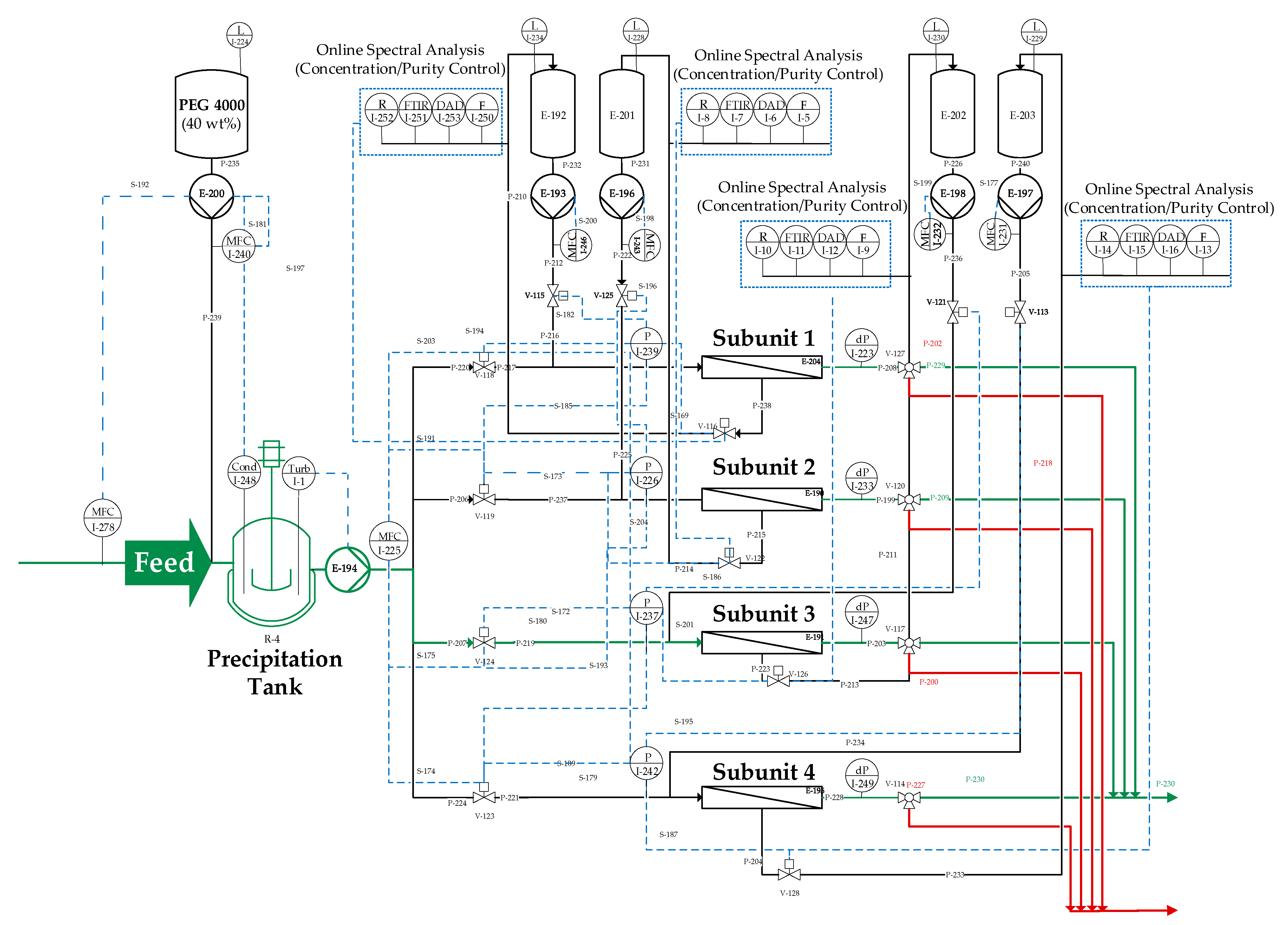Figure 19 shows the flow sheet of the complete unit including the proposed online measurement technique (online spectral analysis) as well as pressure sensors (P) and mass flow controllers (MFC).

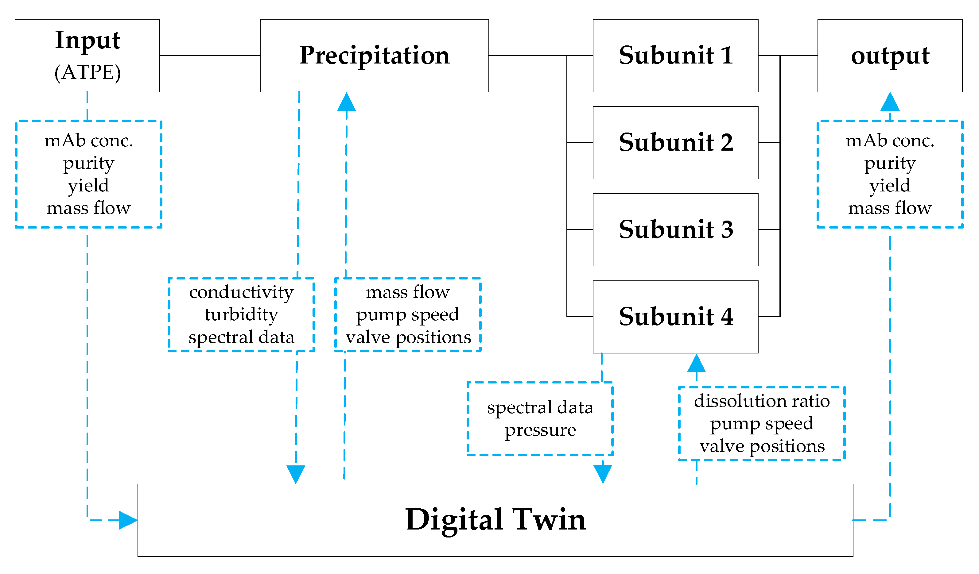
All online measured values are fed back into the digital twin. Figure 20 shows a simplified illustration of the described APC concept. The blue dashed lines represent the signal connection between precipitation unit and digital twin. Hereby, the signal direction is indicated by the arrows. The adjacent boxes show the process parameters that are exchanged between the model and the precipitation unit. The online measurement train between ATPE and precipitation unit determines the initial parameters (IgG concentration, yield, and purity) for the precipitation unit. Further, the mass flow of the incoming feed is measured. Precipitation itself is a concentration independent process [52], therefore, the needed precipitant is calculated dependent on the incoming mass flow. Based on the MFC information the model calculates the mass flow rate of the precipitant (PEG 4000) and the speed of the PEG pump (E-200 in) is aligned. A conductivity probe in the precipitation tank is used to monitor the ratio between feed and precipitant. In the event of a deviation the speed of the PEG pump is adjusted to compensate the mass flow variation of the feed. The turbidity probe monitors the precipitation progress and ensures that the precipitation is completed, and no more antibody remains dissolved in the supernatant. Once the defined level in the precipitation tank is reached and the precipitation is finished (monitored trough turbidity), valves are opened, and filtration starts with the fist module (marked as Subunit 1 in). Filtration is performed in dead-end mode to avoid product loss and to deposit all precipitates on the membrane surface. Pressure sensors are used to measure the transmembrane pressure to prevent pressure peaks out of the operation range of the filters. At a critical pressure valves are switched, and the dispersion is directed to the next module.

The first loaded module moves on to the next phase, the dissolution of the precipitates. Here, the input variables from ATPE and the specification of the final concentration are used to determine model-based the required buffer volume in dissolution. Dissolution is performed in the membrane module by tangentially overflowing the surface area at a high flow rate. Dead-end filtration has compressed the precipitates, which leads to decelerated dissolution kinetics. The experiments have shown that a time of about 14 h is required to reach a yield of >90% antibody recovery after dissolution. The dissolution circuit also contains the measuring equipment described above, which controls the speed of the dissolution buffer pump as well as the valves to the product tank. As soon as the dissolution of the antibody has reached a stationary value, the dissolution is terminated. The module moves on to regeneration, to be ready for the next filtration phase.

4.2. Precipitation Subunit Modeling

The presented simulation study is accomplished with the digital twin presented for one subunit as shown in Figure 1. This study aims to demonstrate that the precipitation unit can react to process variations during manufacturing and is able to provide a constant output concentration. The simulation studies are executed in Aspen Custom Modeler™ (ACM).

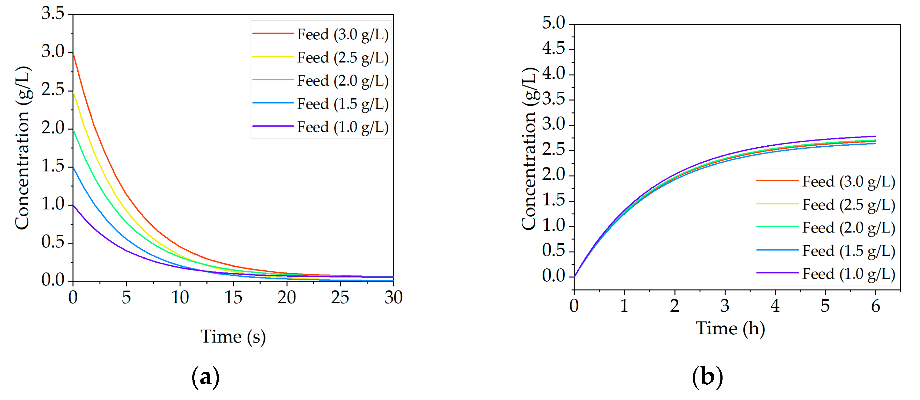
In the initial simulation study feed titers ranging from 1 to 3 g/L have been simulated, since this is a realistic fluctuation for the described laboratory process. The final mAb concentration of 3 g/L is attempted to be achieved after dissolution. Figure 21a shows the concentration decrease in the precipitation step over process time for varying incoming feed concentrations. It becomes obvious that complete precipitation results within a few seconds after PEG addition. Thus, concentration variations do not affect the precipitation step if the precipitation conditions of 12 wt % PEG are maintained. Furthermore, a concentration adjustment in this step is not desirable since the aim is to fully precipitate the target and to prevent product loss. This occurs as soon as a quantity of the antibody remains dissolved in the supernatant. Since precipitation takes place in a stirred tank, temporary concentration fluctuations are mitigated and not directly passed on to filtration. An unstable feed concentration does influence the precipitated mass though. Varying mass of precipitates would lead to extended or shortened filtration time. Hence, concentration adjustments must be addressed in dissolution. To provide the constant output concentration the dissolution ratio is modified Figure 21b, a constant mAb concentration of around 2.7 g/L (± 0.05) in the dissolved output can be observed. This was achieved with the before mentioned adjustment of the dissolution ratio. This simulation study demonstrated that precipitation is capable to provide a constant concentration which is important for the following chromatography.

4.3. Reaction to Process Disturbances

To investigate the response capabilities of the unit operation to eventual process deviations, three theoretical process variations are simulated that are realistic variations for the described process. The simulation studies are labeled as scenario 1–3:

• Concentration variations
• Mass flow fluctuations
• Purity changes

As mentioned before product titer and purity can variate in a bioprocess due to growth rates or other complex conditions. Mass flow deviation may occur through pump failures or can be caused during ATPE. The expected values for the process are a mAb titer of 2 g/L, an ATPE mass flow rate of 1 g/min as well as the purity after ATPE (15 ± 2%). All process variations are discussed for the precipitation step and the dissolution separately.

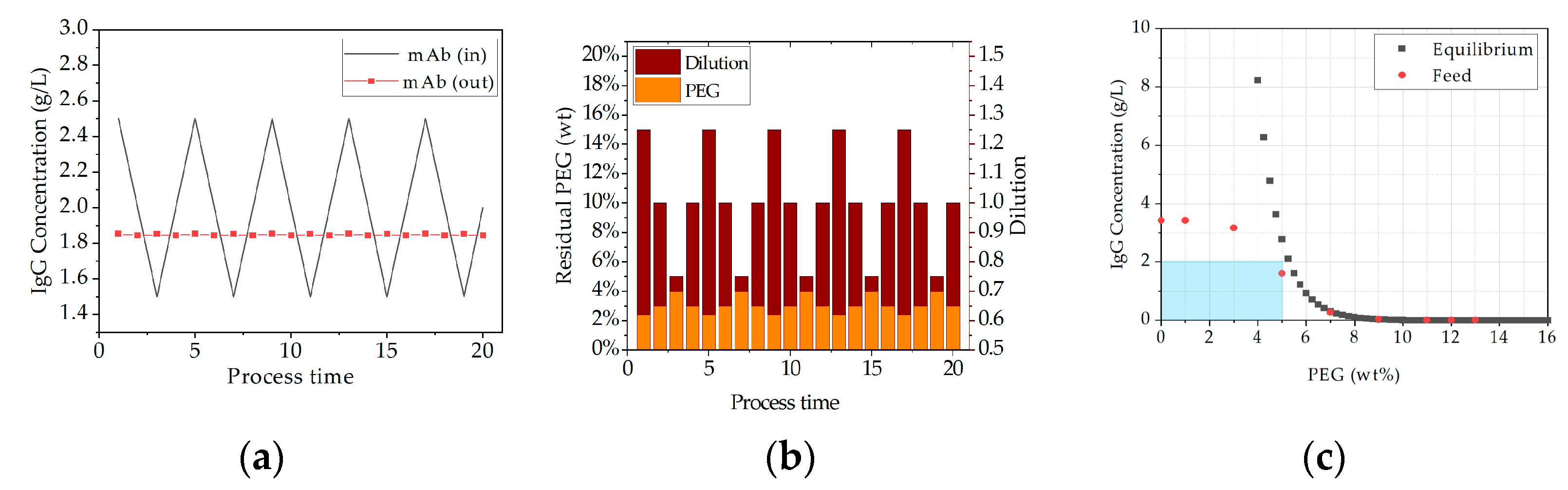
The first study within scenario one includes the proposed APC concept to simulate a process fluctuation during continuous operation. For this purpose, a periodic concentration change is used as input signal, which fluctuates from 2.5 to 1.5 g/L. A final concentration of 2 g/L is attempted to be achieved after dissolution. Figure 22a demonstrates the simulation results with and without the APC. Without APC the concentration fluctuations are still obvious after dissolution (grey line). But if the dissolution ratio is adjusted through APC the unit can provide a constant mAb concentration of 1.85 (±0.03 g/L) besides any feed fluctuations (red line). Figure 22b visualizes which parameters must be controlled to ensure a consistent concentration. By adjusting the dissolution ratio (brown columns), either slight concentration of the target component or dilution is achieved to result in a constant output concentration. Associated with this is the change in the residual PEG content (orange columns), which can become limiting due to the thermodynamic equilibrium. This is shown in Figure 22c. The grey line depicts the equilibrium concentration of mAb in presence of an increasing PEG content. The red line represents the solubility of IgG in the feed at different PEG concentrations. The blue shaded area indicates the thermodynamically given operating window, within which the laboratory process can be carried out without. Outside of this operation window limitation by PEG occur during redissolution, which leads to product loss. It becomes obvious that a PEG content above 5 wt % limits the resolution of the antibody (see Figure 22c). In an industrial environment, this window must be selected the more narrowly, due to higher titers that are achieved during Upstream processing. Then, the remaining PEG should not exceed a proportion of 3 wt % [13].

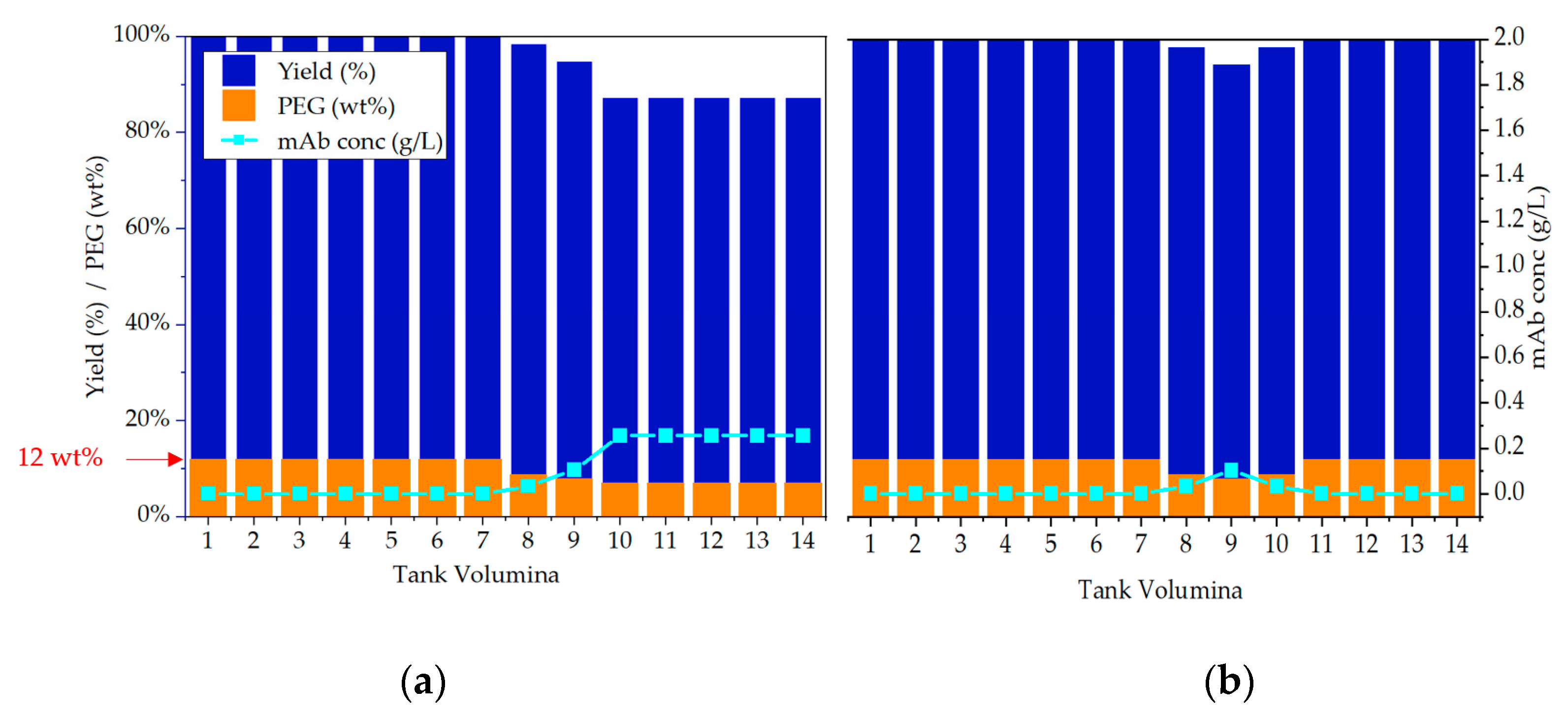
In the following section simulation studies regarding scenario two, which address mass flow fluctuations, are presented. Initial simulations have shown that volume fluctuations mainly affect the precipitation step. This occurs because the supernatant is removed by filtration and is, therefore, not passed on to the subsequent dissolution. The simulations have also shown that an elevated PEG content does not lead to yield loss, hence, here only the simulation results in case of an insufficient PEG content are shown. points out the potential failure mode with and without the integration of the proposed APC. Changes in the mass flow impact the present precipitation conditions in the precipitation tank, which are monitored with the conductivity probe. If this disturbance occurs over a longer period than a few seconds a wrong ratio between PEG and light phase would be present in the precipitation tank in relation to its residence time. This case is shown in Figure 23a. During operation, the required PEG content of 12 wt % can no longer be maintained (orange columns), which leads to an increase in the equilibrium concentration of IgG (light blue line). As a result, the target component no longer precipitates completely, and a residual portion remains dissolved which are potential yield losses. This dissolved residue would then be discarded through dead-end filtration which is not desirable. This loss is indicated by the decreased yield in the precipitation step (blue columns).

The second simulation study within scenario two addresses also the continuous operation with integrated APC (see Figure 23b). In this case the PEG mass flow is adjusted as soon as the PEG content is decreasing in the precipitation tank. This results in a brief increase of the equilibrium concentration in relation to the residence time (10 min). Afterwards the operating point with the correct equilibrium concentration is reached again, and thus no more product loss occurs. For this study the difference in yield loss is about 13%.

Scenario three was also investigated, but the compensation of a purity changes in the feed is not possible with the presented precipitation unit. The reason for this is that in the precipitation and dissolution step, an equilibrium is reached. It is not possible to influence the extent to which the side components precipitate or redissolve. Hence, no specific control parameter is available to adjust the purity. Nonetheless, the purity gain of this unit operation is enormous. Starting with an initial purity of 15 ± 2% after ATPE the purity is increased to an extent of 85 ± 5% after dissolution. This purity increase measured with SEC chromatography is previously shown in Figure 7.

Concluding it can be said that concentration and mass flow changes can both be compensated in the precipitation unit within a short time span of a few seconds. This is reached through the integration of the proposed APC. Nonetheless, both failure modes cannot be compensated at once, since a constant mAb output concentration is always accompanied by a fluctuation in the output mass flow. So, either concentration can be compensated or the mass flow. All simulation results are summarized in

Table 2. Summary of simulations results.

Scenario (Deviation ± 50%)	Precipitation	Dissolution
Concentration (a) high (b) low	(a + b) Concentration deviation does not have impact on precipitation. → Precipitant mass flow is calculated based on Feed mass flow	(a) Volume dissolution buffer ↑ (b) Volume dissolution buffer ↓ → Solubility limits volume reduction of dissolution buffer downwards → Control Parameter: mass flow → Control Strategy: pump speed
Feed mass flow (a) Increased (b) decreased	(a) PEG Stream ↑ (b) PEG Stream ↓ → Control Parameter: Conductivity → Control Strategy: pump speed	(a) Volume dissolution buffer ↓ (b) Volume dissolution buffer ↑ → Control Parameter: Conductivity → Control Strategy: pump speed
Purity of IgG (a) Increased (b) decreased	Precipitation does not have an impact on purity of the target	Dissolution does not have an impact on purity of the target

.

5. Conclusions

It has been shown that precipitation as a unit operation is very robust and achieves a high depletion of the side components due to the mode of operation. The purity is increased from 15 ± 2% after ATPE to 85 ± 5% after dissolution. The remaining impurities mainly consisting of LMWs and PEG, which can be separated easily in flow-through mode in the following chromatography (IEX). The dissolution buffer is at the same time the running buffer of the subsequent chromatography, which makes the transfer simple and no additional diafiltration is required. All in all, shows that precipitation is suitable for purification of mAb and can be ideally integrated into the alternative manufacturing process between extraction and chromatography. A further advantage is that no cost-intensive materials or equipment are needed. On the contrary, all used components and equipment devices are already standard in industry and can simply be scaled to other scales.

Moreover, the feasibility of using online measurement technology has been demonstrated within the framework of the PAT initiative. All detectors delivered very good results in the analysis of product concentration. However, the best result was achieved by Raman, which reliably detected product concentration and purity online. Furthermore, the combination of DAD and Raman has been tested, which is a recommended extension due to the orthogonal measurement methods, resulting in higher process robustness. Finally, in a simulation study, which has been performed with aid of a digital twin, the online measurement data have been successfully used to control the process. This led to minimized yield losses at potential feed flow or concentration fluctuations. Further studies will focus on continuous operation mode and transfer the process to other biologics such as fragments, peptides, pDNA and VLPs at the Institute.