Integrating Machine Learning, Radio Frequency Identification, and Consignment Policy for Reducing Unreliability in Smart Supply Chain Management

Abstract

Adopting smart technologies for supply chain management leads to higher profits. The manufacturer and retailer are two supply chain players, where the retailer is unreliable and may not send accurate demand information to the manufacturer. As an advanced smart technology, Radio Frequency Identification (RFID) is implemented to track and trace each product’s movement on a real-time basis in the inventory. It takes this supply chain to a smart supply chain management. This research proposes a Machine Learning (ML) approach for on-demand forecasting under smart supply chain management. Using Long-Short-Term Memory (LSTM), the demand is forecasted to obtain the exact demand information to reduce the overstock or understock situation. A measurement for the environmental effect is also incorporated with the model. A consignment policy is applied where the manufacturer controls the inventory, and the retailer gets a fixed fee along with a commission for selling each product. The manufacturer installs RFID technology at the retailer’s place. Two mathematical models are solved using a classical optimization technique. The results from those two models show that the ML-RFID model gives a higher profit than the existing traditional system.

1. Introduction

In supply chain management (SCM), each manufacturer observes customer demand to decide production quantity. If the demand is uncertain, either overstock or understock situations occur at the stockholder. The supply chain players play an essential role in this situation. Demand uncertainty can be caused if the players are unreliable or if they are not exchanging proper information between them. Depending on the demand, the manufacturer produces products and sends those products to the retailer for selling. The retailer controls the overall inventory and sends money to the manufacturer after selling the products. However, sometimes, the retailer is untrustworthy. The retailer does not provide accurate information to the manufacturer. In this case, a consignment policy is applied to reduce the information asymmetry between supply chain players. Additionally, using smart technology, such as RFID, gives an extra advantage for getting real-time information about the products in the inventory. Incorporating these features takes supply chain management to an advanced level as compared to traditional systems.

A consignment policy is an approach where the manufacturer manages the financial part, and the retailer maintains the operational functions. In this policy, the manufacturer acts as a leader, and the retailer acts as a follower. The overall inventory is controlled by the manufacturer only. The retailer sells those products and sends its revenue to the manufacturer ([1,2]). The manufacturer provides specific incentives to the retailer for each product sold ([3]). By a mutual agreement between both the players, unsold products are returned to the legal owner. Additionally, manufacturing the products needs to be perfect to improve the quality of the products (Sarkar and Sarkar [4]). A service-level constraint for quality improvement was introduced by Moon et al. [5]. By implementing a service-level restriction in this supply chain model, the product quality is improved by optimizing the model through a distribution-free approach ([6]). This improved service strategy for the consignment stock is applied in this research to extend the traditional model to gives a higher profit.

A typical warehouse has certain limitations when tracking and tracing products, which causes information asymmetry with unnecessary time consumption. As an advanced smart technology, RFID is implemented to observe every single movement of each product in the inventory ([7]). The real-time tracking, tracing, and inspecting of products are done in a completely automatic procedure with minimum human interaction and minimum labor cost. This automation policy allows for smart supply chain management in the model ([8]). Another profitable strategy for using RFID is that RFID tags can reuse, and some amount of data can be stored if needed ([9]). RFID tags are attached to products and traced by scanners mounted in the warehouse. The real-time information of each product is sent to a server, and users can get information about the inventory from the server by using a computer or smartphone. RFID implementation in supply chain management for optimizing unreliability and increasing the overall profit was briefly described by Biswal et al. [10].

Demand forecasting plays a crucial role in this smart supply chain model. When the retailer is unreliable and does not send accurate demand information to the manufacturer, demand uncertainty arises ([11]). Thus, the manufacturer cannot predict the exact market demand. In this situation, the holding cost or shortage cost increases, and the supply chain management system’s total profit decreases ([12]). Based on previous demand data, LSTM is applied to forecast future demand. A multi-layer LSTM network was proposed by Abbasimehr et al. [13], which can predict volatile demand data by considering various combinations of LSTM hyperparameters for a provided time series. Using the expected demand leads to higher profit over the traditional model ([14]). By the forecasted demand, an essential competitive advantage is created for generating superior business performance ([15]). As information asymmetry makes this type of smart supply chain management unreliable, this study maximizes the entire smart supply chain’s total profit by minimizing the unreliability between supply chain players.

In the existing traditional system, the retailer is unreliable and does not provide accurate inventory information to the manufacturer. As a result, information asymmetry arises between supply chain players. The manufacturer does not have precise demand information for future production. The main contribution of this research is forecasting the future demand using an LSTM method and incorporating RFID and a consignment policy into the traditional model where the profit will be higher than the traditional system. As information asymmetry arises in the traditional model, RFID is implemented to get accurate information about the inventory on a real-time basis for reducing unreliability. A consignment policy is applied in which the manufacturer controls the overall inventory, and the retailer sells the products and sends the money to the manufacturer. The manufacturer provides a fixed amount of money and a commission to the retailer for selling each product. As the demand is forecasted using LSTM, the manufacturer produces goods based on the predicted future demand ([16]). In this case, the holding cost or the shortage cost is minimized, and the total profit is much higher than the existing traditional model.

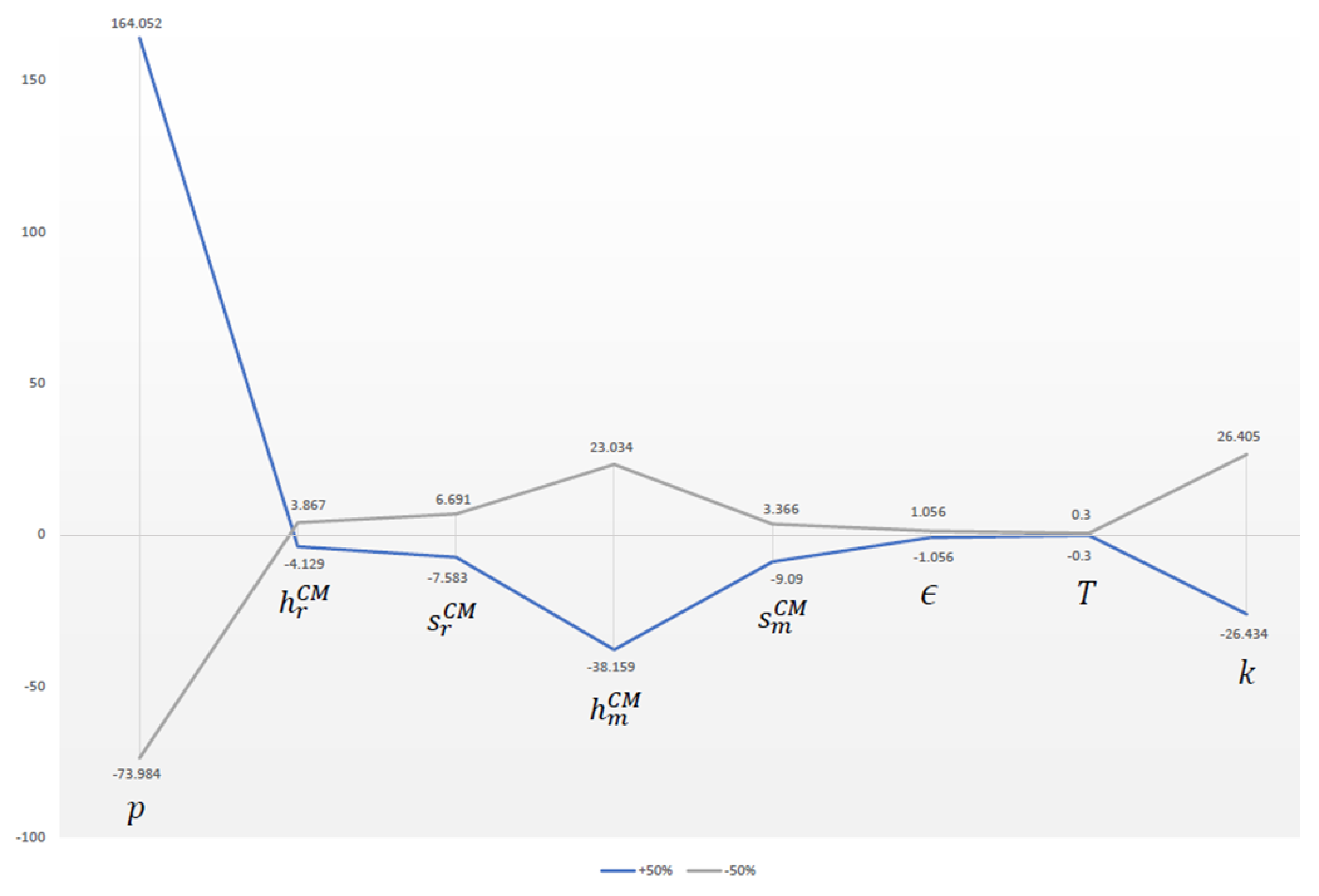
Section 1 represents the introduction and contribution of authors along with problem definition, assumptions, and notation of this research. The rest of the research is designed as follows. Section 2 signifies the traditional model part. The modeling part of ML-RFID model is formulated in Section 3. The results of this research are described in Section 4 followed by a sensitivity discussion on the parameters. Section 5 contains managerial implications and Section 6 concludes this research.

1.1. Contribution of Authors

An author’s contribution table based on keywords and literature is described in

Table 1. Author’s contribution table.

Author(s)	Smart	Inventory	Unreliability	RFID	Consignment	Machine
	SCM	Control			Policy	Learning
Scarf [17]		√
Gallego and Moon [18]		√
Ouyang et al. [19]		√
Dias et al. [20]				√
Sarac et al. [21]		√
Kim and Glock [22]				√
Sarkar et al. [23]		√			√
Guchhait et al. [24]		√	√	√
Sardar and Sarkar [25]		√	√	√	√
This research	√	√	√	√	√	√

which clearly illustrates the contrast of this research with previous research.

1.2. Problem Definition, Assumptions, and Notation

The problem definition of this study is demonstrated in this section. The assumptions and the notation used to mathematically validate the proposed model are described below.

1.2.1. Problem Definition

In this study, the difference between the traditional and ML-RFID models in smart supply chain management is described for reducing unreliability. Two supply chain players, i.e., the manufacturer and the retailer, play an essential role but have asymmetric power. Due to the unreliable retailer, the Stackelberg game approach is applied to determine the decision-maker. A future demand distribution is incorporated, dependent on the service based on a machine learning technique, i.e., LSTM. Under a consignment policy, a fixed fee is given to the retailer by the manufacturer to implement RFID, which reduces the players’ information asymmetry by providing accurate information about the inventory. The retailer sells the products, sends the revenue to the manufacturer, and then gets a commission to sell each product. This research gives a higher profit than the traditional model after implementing RFID and a consignment policy with machine learning, providing smart supply chain management in this supply chain.

1.2.2. Assumptions

The following assumptions are used for this research.

• A supply chain management is considered with manufacturer and retailer as two players.
• Demand depends on the service b, and it is a decision variable.
• In the traditional model, the inventory is controlled by the retailer. In the ML-RFID model, the manufacturer controls the inventory by giving a fixed fee along with a commission to the retailer for each product sold.
• The lead time demand does not follow a known probability distribution function but it has a known value of the mean and standard deviation ([26]).
• As the retailer is unreliable, the manufacturer installs RFID technology at the retailer’s place to get real-time information about the inventory ([24]).
• The demand dataset consists of ten years of data, and $65\%$ of the data are taken as the training dataset while the remaining $35\%$ are taken as the test dataset.
• The data in the test set do not exist in the train set and the demand is always greater than zero.
• Using Stackelberg game theory, the manufacturer acts as a leader and controls the inventory. The retailer acts as a follower of the manufacturer ([27]).

1.2.3. Notation

The notation associated with this research is is attached in Appendix A.

2. Traditional Model

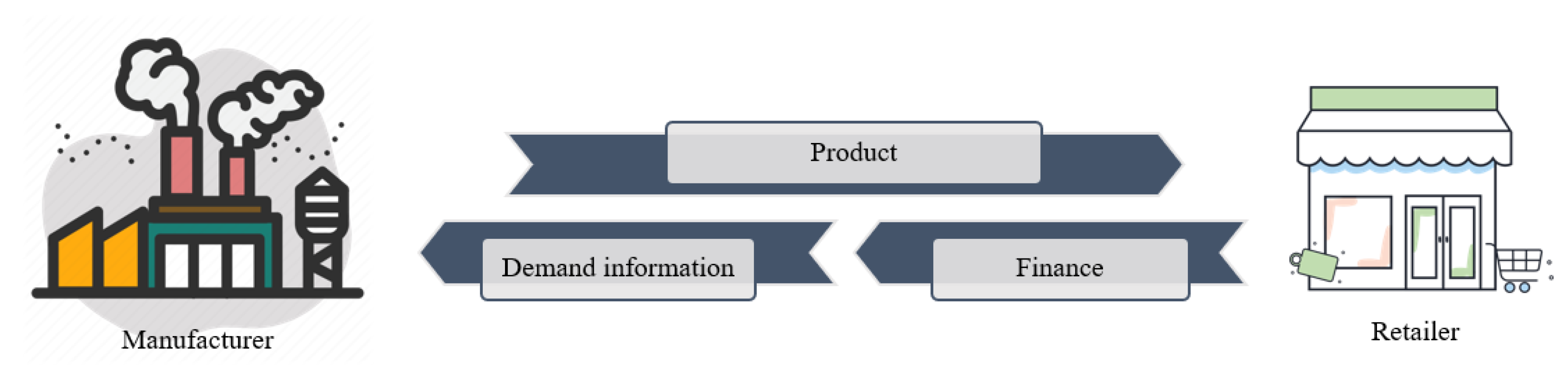
The traditional model is a conventional model where the manufacturer makes products and sends them to the retailer. In this model, the inventory is controlled by the retailer. The manufacturer receives demand information and the money after selling products from the retailer. This traditional model has some limitations related to information asymmetry. When the retailer is unreliable and does not send accurate demand information to the manufacturer, the overstock or understock situation arises.

Further, to reduce its environmental impact, each industry must follow some legislative regulations. Each industry mitigates its carbon footprint by incorporating a cap and trade policy ([28]). For the approach, a measurement of the environmental effect is considered in this model ([29]). This model consists of three subsections: the retailer’s traditional model, the manufacturer’s classic model, and the total expected profit for the conventional model. Figure 1 represents the process diagram for the traditional model.

2.1. Retailer’s Traditional Model

In the traditional model, the retailer’s holding cost of the total product’s inventory is incurred. The entire lot is purchased at a wholesale price by the retailer from the manufacturer. Thus, the retailer maintains the products’ proprietorship, and products are sold to the customer at a selling price. In this model, the manufacturer no longer has responsibility for the products. The manufacturer does not acquire holding costs for a single product after making the delivery to the retailer. The demand of the retailer is $D=a{b}^{\gamma }{e}_{\eta }^{\beta }$, where a is the scaling parameter, $\gamma$ and $\beta$ are shape parameters, b is the service provided to the customers, and $e_{\eta }$ is the measurement of the environmental effect.

The total profit of the retailer under the traditional model is:

$$E\left({\Pi }_r^{TM}\right)=\left\{\begin{array}{cc}pa{b}^{\gamma }{e}_{\eta }^{\beta }-\omega Q_r-h_r^{TM}{(Q_r-a{b}^{\gamma }{e}_{\eta }^{\beta }L)}^{+}-C\left(L\right)-\frac{\rho e_{\eta }^2}{2};\hfill & \hfill a{b}^{\gamma }{e}_{\eta }^{\beta }\le Q_r\\ (p-\omega )Q_r-s_r^{TM}{(a{b}^{\gamma }{e}_{\eta }^{\beta }L-Q_r)}^{+}-C\left(L\right)-\frac{\rho e_{\eta }^2}{2};\hfill & \hfill Q_r<a{b}^{\gamma }{e}_{\eta }^{\beta }\end{array}\right\}.$$

(1)

As the retailer is unreliable, the manufacturer does not get proper demand information. Thus, an overstock or understock situation arises in this conventional model. The necessity of the lead time demand information is essential to calculate the holding or shortage during the lead time period. According to Gallego and Moon [18], without having distribution information, one can easily calculate the expected holdings or shortages during the lead time demand using a lemma that places an upper bound. Using this lemma, one has the following:

Lemma 1.

(i)The expected quantity for overstock:

$$\begin{array}{ccc}\hfill E{(Q_r-a{b}^{\gamma }{e}_{\eta }^{\beta }L)}^{+}& \le & \frac{1}{2}\left[\sqrt{{\delta }^2+{(Q_r-a{b}^{\gamma }{e}_{\eta }^{\beta }L)}^2}-(a{b}^{\gamma }{e}_{\eta }^{\beta }L-Q_r)\right].\hfill \end{array}$$

(2)

(ii) The expected quantity for understock:

$$\begin{array}{ccc}\hfill E{(a{b}^{\gamma }{e}_{\eta }^{\beta }L-Q_r)}^{+}& \le & \frac{1}{2}\left[\sqrt{{\delta }^2+{(Q_r-a{b}^{\gamma }{e}_{\eta }^{\beta }L)}^2}-(Q_r-a{b}^{\gamma }{e}_{\eta }^{\beta }L)\right].\hfill \end{array}$$

(3)

Using Equations $\left(2\right)$ and $\left(3\right)$, the expected profit for the retailer is calculated for Equation $\left(1\right)$, and it can be written as:

$$\begin{array}{ccc}\hfill E\left({\Pi }_r^{TM}\right)& =& p(a{b}^{\gamma }{e}_{\eta }^{\beta }+Q_r)-C\left(L\right)-\frac{\rho e_{\eta }^2}{2}-\omega Q_r-\frac{h_r^{TM}}{2}\left[\sqrt{{\delta }^2+{(Q_r-a{b}^{\gamma }{e}_{\eta }^{\beta }L)}^2}-(a{b}^{\gamma }{e}_{\eta }^{\beta }L-Q_r)\right]\hfill \\ & & -\frac{s_r^{TM}}{2}\left[\sqrt{{\delta }^2+{(Q_r-a{b}^{\gamma }{e}_{\eta }^{\beta }L)}^2}-(Q_r-a{b}^{\gamma }{e}_{\eta }^{\beta }L)\right].\hfill \end{array}$$

(4)

2.2. Manufacturer’s Traditional Model

The manufacturer follows the optimized decision in the traditional model. The revenue of the manufacturer is $\omega Q_r$ and the manufacturing cost is $k{Q}_r$ where the unit production cost is denoted by k. The expected profit of the manufacturer under the traditional model is:

$$\begin{array}{ccc}\hfill E\left({\Pi }_m^{TM}\right)& =& \omega Q_r-k{Q}_r\hfill \\ & =& (\omega -k)Q_r.\hfill \end{array}$$

(5)

2.3. Total Expected Profit for the Traditional Model

By adding Equations $\left(4\right)$ and $\left(5\right)$, the total expected total profit under traditional model is

$$\begin{array}{ccc}\hfill E\left({\Pi }_j^{TM}\right)& =& E\left({\Pi }_r^{TM}\right)+E\left({\Pi }_m^{TM}\right)\hfill \\ \hfill & =& p(a{b}^{\gamma }{e}_{\eta }^{\beta }+Q_r)-C\left(L\right)-\frac{\rho e_{\eta }^2}{2}-k{Q}_r-\frac{h_r^{TM}}{2}\left[\sqrt{{\delta }^2+{(Q_r-a{b}^{\gamma }{e}_{\eta }^{\beta }L)}^2}-(a{b}^{\gamma }{e}_{\eta }^{\beta }L-Q_r)\right]\hfill \\ & & -\frac{s_r^{TM}}{2}\left[\sqrt{{\delta }^2+{(Q_r-a{b}^{\gamma }{e}_{\eta }^{\beta }L)}^2}-(Q_r-a{b}^{\gamma }{e}_{\eta }^{\beta }L)\right].\hfill \end{array}$$

(6)

According to Sardar and Sarkar [25], the maximum profit can be obtained by taking the derivative of Equation $\left(6\right)$ with respect to $Q_r$, L, b, and $e_{\eta }$. Now, the optimum values for the decision variables are:

$$\begin{array}{ccc}\hfill \Rightarrow Q_r^{*}& =& a{b}^{\gamma }{e}_{\eta }^{\beta }L+\frac{\{2(p-k)-h_r^{TM}+s_r^{TM}\}\delta }{\sqrt{{\left(h_r^{TS}+s_r\right)}^2-{\{2(p-k)-h_r^{TS}+s_r\}}^2}}.\hfill \end{array}$$

$$\begin{array}{ccc}\hfill \Rightarrow L^{*}& =& \frac{1}{a{b}^{\gamma }{e}_{\eta }^{\beta }}\left[Q_r-\frac{{\delta }^2{\left(\frac{2c_i}{a{b}^{\gamma }{e}_{\eta }^{\beta }}+s_r^{TM}-h_r^{TM}\right)}^2}{{\left(h_r^{TM}+s_r^{TM}\right)}^2-{\left(\frac{2c_i}{a{b}^{\gamma }{e}_{\eta }^{\beta }}+s_r^{TM}-h_r^{TM}\right)}^2}\right].\hfill \end{array}$$

$$\begin{array}{ccc}\hfill \Rightarrow b^{*}& =& {\left[\frac{1}{a{e}_{\eta }^{\beta }L}\left\{Q_r-\frac{\delta (\frac{2p}{L}+h_r^{TM}-s_r^{TM})}{\sqrt{{\left(\frac{2p}{L}+h_r^{TM}-s_r^{TM}\right)}^2-{\left(h_r^{TM}+s_r^{TM}\right)}^2}}\right\}\right]}^{\frac{1}{\gamma }}.\hfill \end{array}$$

$$\begin{array}{ccc}\hfill \Rightarrow e_{\eta }^{*}& =& \frac{\beta pa{b}^{\gamma }{e}_{\eta }^{\beta -1}-(h_r^{TM}+s_r^{TM})\left[\frac{\frac{a{b}^{\gamma }\beta e_{\eta }^{\beta -1}L(Q_r-a{b}^{\gamma }{e}_{\eta }^{\beta }L)}{{\{{\delta }^2+{(Q_r-a{b}^{\gamma }{e}_{\eta }^{\beta }L)}^2\}}^{\frac{1}{2}}}+a{b}^{\gamma }\beta e_{\eta }^{\beta -1}L}{2}\right]}{\rho }.\hfill \end{array}$$

3. Integrating ML, RFID, and Consignment Policy to Reduce Unreliability (ML-RFID Model)

In the ML-RFID model, products are sent to the retailer by the manufacturer, and the retailer maintains the inventory. The retailer does not have to pay any money until the products are sold. In a consignment policy, two different segments are present. In the first segment, the inventory prepares for receiving the products. In the second segment, the retailer sells the products, and the revenue is sent to the manufacturer. 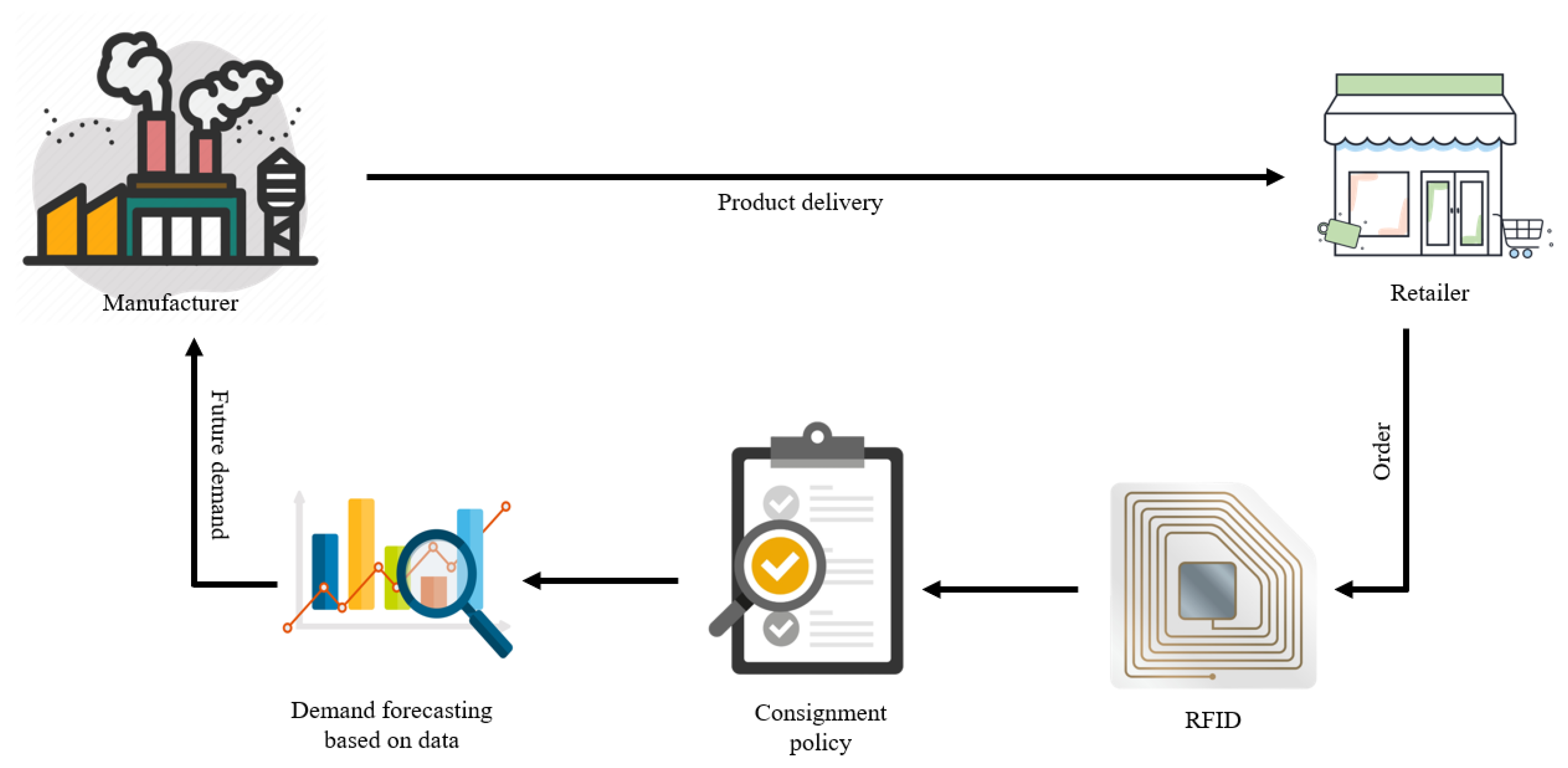The Stackelberg game approach is used where the manufacturer behaves as a leader by controlling the overall inventory, and the retailer acts as a follower ([30]). The manufacturer maintains the consignment stock and sends a commission to the retailer for each product sold with a fixed fee; thus, the retailer’s revenue is generated. Implementation of RFID reduces the unreliability by real-time tracking of each product in the inventory, which leads to higher profits than the traditional model. LSTM is used to remove the uncertainty of demand so that the holding cost and shortage cost are minimized, increasing the profit of the whole smart supply chain management strategy. The implementation of demand forecasting over the ML-RFID model is shown in Figure 2.

3.1. Forecasting Future Demand to Remove Uncertainty

LSTM can forecast time series data as an extension of the Recurrent Neural Network (RNN). Long-range time-dependent information can store in LSTM by correctly mapping both the input and output data ([31]). LSTM consists of an input gate, a forget gate, an output gate, and internal cells ([32]). Those gates and cells control the flow of information. In the LSTM method, the training and test datasets are taken in some specific ratio. The demand patterns are similar for each day. 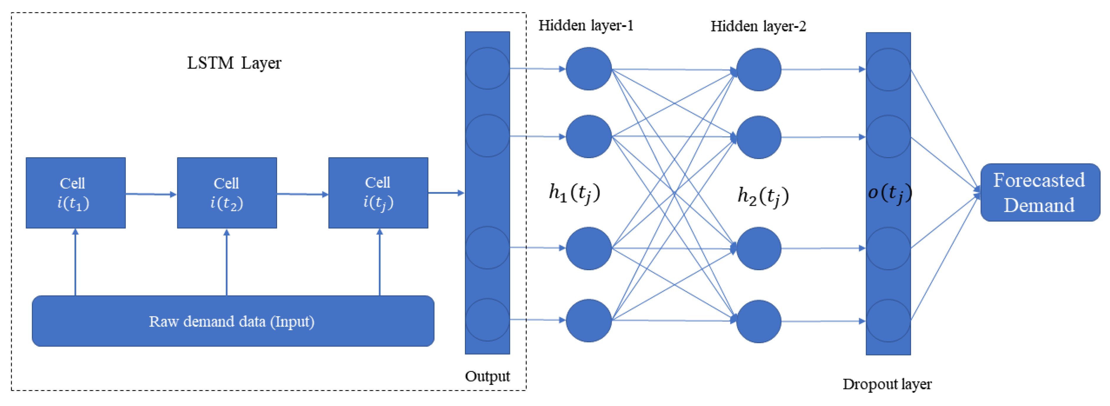A preprocessing step is done by assigning different weights to the input data, affecting the forecasted data ([33]). For LSTM, a dataset matrix is formed by converting the array value, followed by reshaping the inputs for predicting and checking the performance matrices. Figure 3 is a pictorial representation of the LSTM architecture used in demand forecasting.

Formulation of LSTM

Suppose, there is a time series dataset of length $t_j$ that consists of $\{i\left(t_1\right),i\left(t_2\right),i\left(t_3\right),\cdots ,i\left(t_j\right)\}$ which should first be preprocessed.

The time series $i\left(t_j\right)$ is normalized and the result is given below:

$$\begin{array}{c}\hfill i\left(t_j\right)=\frac{i\left(t_j\right)-min\left(i\right)}{max\left(i\right)-min\left(i\right)}\end{array}$$

(7)

In Equation $\left(7\right)$, $max\left(s\right)$ and $min\left(s\right)$ are the maximum and minimum values of s.

Reshaping the data is done in this step followed by splitting the data into a training set and test set. The training set is considered as the input of the LSTM model and the prediction evaluation in terms of the performance metrics is done in the test set.

$i\left(t_j\right)$ is the input demand of the first LSTM hidden layer with previous state $h_1\left(t_{j-1}\right)$, which gives the forecasted output demand at time $t_{j-1}$. The output value of the first layer is $h_1\left(t_j\right)$. The output forecasted demand of the first layer is used by the second hidden layer with the previous output. The output of hidden layer $h_1\left(t_j\right)$ is used with the previous state to calculate the output value of $h_2\left(t_j\right)$. Then, $h_2\left(t_{j-1}\right)$ becomes the input demand of the next hidden layer along with output value $h_2\left(t_j\right)$. This process continues in each layer by calculating the time series demand data prediction and passing the value to the next layer until the last layer computes the final forecasted demand. The forecasted output for the output gate is denoted by $o\left(t_j\right)$ at time $t_j$.

3.2. Retailer’s Expected Profit for the ML-RFID Model

The retailer carries the product’s inventory but does not hold the total product’s inventory holding cost. This setup functions as a follower in the Stackelberg game approach. Only the operation parts, such as the stock handling and storage area, are carried by the retailer, which means the holding cost $\left(h_r^{CM}\right)$ and the shortage cost $\left(s_r^{CM}\right)$ are carried by the retailer. To remove the unreliability of the traditional model, RFID is introduced and the cost for RFID implementation $\left(Q_rϵ\right)$ is borne by the retailer. The retailer also receives an amount of money $\left(T\right)$ for installing the RFID system from the manufacturer. The retailer agrees to a contract and makes revenue from the commission and the fixed fee given by the manufacturer.

Therefore, the retailer’s expected total profit for the ML-RFID model is

$$\begin{array}{c}\hfill E\left({\Pi }_r^{CM}\right)=\left\{\begin{array}{cc}\theta a{b}^{\gamma }{e}_{\eta }^{\beta }-h_r^{CM}{(Q_r-a{b}^{\gamma }{e}_{\eta }^{\beta }L)}^{+}-C\left(L\right)+A-Q_rϵ-T-\frac{\rho e_{\eta }^2}{2};\hfill & \hfill a{b}^{\gamma }{e}_{\eta }^{\beta }\le Q_r\\ \theta Q_r-s_r^{CM}{(a{b}^{\gamma }{e}_{\eta }^{\beta }L-Q_r)}^{+}-C\left(L\right)+A-Q_rϵ-T-\frac{\rho e_{\eta }^2}{2};\hfill & \hfill Q_r<a{b}^{\gamma }{e}_{\eta }^{\beta }\end{array}\right\}.\end{array}$$

Now, using Equations $\left(2\right)$ and $\left(3\right)$, the expected profit of the retailer can be written as

$$\begin{array}{ccc}\hfill E\left({\Pi }_r^{CM}\right)& =& \theta (a{b}^{\gamma }{e}_{\eta }^{\beta }+Q_r)-C\left(L\right)+A-Q_rϵ-T-\frac{\rho e_{\eta }^2}{2}\hfill \\ \hfill & & -\frac{h_r^{CM}}{2}\left[\sqrt{{\delta }^2+{(Q_r-a{b}^{\gamma }{e}_{\eta }^{\beta }L)}^2}-(a{b}^{\gamma }{e}_{\eta }^{\beta }L-Q_r)\right]\hfill \\ & & -\frac{s_r^{CM}}{2}\left[\sqrt{{\delta }^2+{(Q_r-a{b}^{\gamma }{e}_{\eta }^{\beta }L)}^2}-(Q_r-a{b}^{\gamma }{e}_{\eta }^{\beta }L)\right].\hfill \end{array}$$

(8)

3.3. Manufacturer’s Expected Profit for the ML-RFID Model

As per the Stackelberg game approach, the manufacturer is the leader. Thus, the ownership of the warehouse is controlled by the manufacturer only. The manufacturing cost of the manufacturer is $k{Q}_r$. The financial part of holding cost $\left(h_m^{CM}\right)$ and shortage cost $\left(s_m^{CM}\right)$ are controlled by the manufacturer over traditional model. The manufacturer also gives a fixed fee $\left(A\right)$ to the retailer.

Therefore, the manufacturer’s expected total profit for the ML-RFID model is

$$\begin{array}{c}\hfill E\left({\Pi }_m^{CM}\right)=\left\{\begin{array}{cc}(p-\theta )a{b}^{\gamma }{e}_{\eta }^{\beta }-k{Q}_r-h_m^{CM}{(Q_r-a{b}^{\gamma }{e}_{\eta }^{\beta }L)}^{+}-A;\hfill & \hfill a{b}^{\gamma }{e}_{\eta }^{\beta }\le Q_r\\ (p-\theta -k)Q_r-s_m^{CM}{(a{b}^{\gamma }{e}_{\eta }^{\beta }L-Q_r)}^{+}-A;\hfill & \hfill Q_r<a{b}^{\gamma }{e}_{\eta }^{\beta }\end{array}\right\}.\end{array}$$

Again, using Equation $\left(2\right)$ and Equation $\left(3\right)$ the expected profit of the manufacturer can be written as

$$\begin{array}{ccc}\hfill E\left({\Pi }_m^{CM}\right)& =& p(a{b}^{\gamma }{e}_{\eta }^{\beta }+Q_r)-\theta a{b}^{\gamma }{e}_{\eta }^{\beta }-\theta Q_r-k{Q}_r-A\hfill \\ \hfill & & -\frac{1}{2}{h}_m^{CM}\left[\sqrt{{\delta }^2+{(Q_r-a{b}^{\gamma }{e}_{\eta }^{\beta }L)}^2}-(a{b}^{\gamma }{e}_{\eta }^{\beta }L-Q_r)\right]\hfill \\ & & -\frac{1}{2}{s}_m^{CM}\left[\sqrt{{\delta }^2+{(Q_r-a{b}^{\gamma }{e}_{\eta }^{\beta }L)}^2}-(Q_r-a{b}^{\gamma }{e}_{\eta }^{\beta }L)\right].\hfill \end{array}$$

(9)

3.4. Total Expected Profit for the ML-RFID Model

By adding Equations $\left(8\right)$ and $\left(9\right)$, the expected total profit under the ML-RFID model can be formulated as:

$$\begin{array}{ccc}\hfill E\left({\Pi }_j^{CM}\right)& =& E\left({\Pi }_r^{CM}\right)+E\left({\Pi }_m^{CM}\right)\hfill \\ \hfill & =& pa{b}^{\gamma }{e}_{\eta }^{\beta }-C\left(L\right)-Q_rϵ-T-\frac{\rho e_{\eta }^2}{2}+p{Q}_r-k{Q}_r-\hfill \\ \hfill & & \frac{1}{2}{h}_r^{CM}\left[\sqrt{{\delta }^2+{(Q_r-a{b}^{\gamma }{e}_{\eta }^{\beta }L)}^2}-(a{b}^{\gamma }{e}_{\eta }^{\beta }L-Q_r)\right]\hfill \\ \hfill & & -\frac{1}{2}{s}_r^{CM}\left[\sqrt{{\delta }^2+{(Q_r-a{b}^{\gamma }{e}_{\eta }^{\beta }L)}^2}-(Q_r-a{b}^{\gamma }{e}_{\eta }^{\beta }L)\right]\hfill \\ \hfill & & -\frac{1}{2}{h}_m^{CM}\left[\sqrt{{\delta }^2+{(Q_r-a{b}^{\gamma }{e}_{\eta }^{\beta }L)}^2}-(a{b}^{\gamma }{e}_{\eta }^{\beta }L-Q_r)\right]\hfill \\ & & -\frac{1}{2}{s}_m^{CM}\left[\sqrt{{\delta }^2+{(Q_r-a{b}^{\gamma }{e}_{\eta }^{\beta }L)}^2}-(Q_r-a{b}^{\gamma }{e}_{\eta }^{\beta }L)\right].\hfill \end{array}$$

(10)

The maximum profit can be obtained by taking the derivative of Equation $\left(10\right)$ with respect to $Q_r$, L, b, and $e_{\eta }$ (see Appendix B).

Now, the optimal values for the decision variables are:

$$\begin{array}{ccc}\hfill \Rightarrow Q_r^{*}& =& a{b}^{\gamma }{e}_{\eta }^{\beta }L+\frac{(2p-2ϵ-2k-h_r^{CM}+s_r^{CM}-h_m^{CM}+s_m^{CM})\delta }{\sqrt{{(h_r^{CM}+s_r^{CM}+h_m^{CM}+s_m^{CM})}^2-{(2p-2ϵ-2k-h_r^{CM}+s_r^{CM}-h_m^{CM}+s_m^{CM})}^2}}.\hfill \end{array}$$

$$\begin{array}{ccc}\hfill \Rightarrow L^{*}& =& \frac{1}{a{b}^{\gamma }{e}_{\eta }^{\beta }}\left[Q_r-\frac{{\delta }^2{(\frac{2c_i}{a{b}^{\gamma }}-h_r^{CM}+s_r^{CM}-h_m^{CM}+s_m^{CM})}^2}{{(h_r^{CM}+s_r^{CM}+h_m^{CM}+s_m^{CM})}^2-{(\frac{2c_i}{a{b}^{\gamma }}-h_r^{CM}+s_r^{CM}-h_m^{CM}+s_m^{CM})}^2}\right].\hfill \end{array}$$

$$\begin{array}{ccc}\hfill \Rightarrow b^{*}& =& {\left[\frac{1}{a{e}_{\eta }^{\beta }L}\left\{Q_r-\frac{\delta (\frac{2p}{L}+h_r^{CM}-s_r^{CM}+h_m^{CM}-s_m^{CM})}{\sqrt{{(\frac{2p}{L}+h_r^{CM}-s_r^{CM}+h_m^{CM}-s_m^{CM})}^2-{(h_r^{CM}+s_r^{CM}+h_m^{CM}+s_m^{CM})}^2}}\right\}\right]}^{\frac{1}{\gamma }}.\hfill \end{array}$$

$$\begin{array}{ccc}\hfill \Rightarrow e_{\eta }^{*}& =& \frac{\beta pa{b}^{\gamma }{e}_{\eta }^{\beta -1}-(h_r^{CM}+s_r^{CM}+h_m^{CM}+s_m^{CM})\left[\frac{\frac{a{b}^{\gamma }\beta e_{\eta }^{\beta -1}L(Q_r-a{b}^{\gamma }{e}_{\eta }^{\beta }L)}{{\{{\delta }^2+{(Q_r-a{b}^{\gamma }{e}_{\eta }^{\beta }L)}^2\}}^{\frac{1}{2}}}+a{b}^{\gamma }\beta e_{\eta }^{\beta -1}L}{2}\right]}{\rho }.\hfill \end{array}$$

4. Experimental Results

The experimental results section of this research along with validation of the model are given below. We have added subsections that describe the results of demand forecasting in Section 4.1, compared the proposed model and the traditional model in Section 4.2, and presented the sensitivity analysis in Section 4.3.

4.1. Forecasting Using LSTM

The demand dataset for forecasting consists of ten years of data. Depending on the complexity and number of features of the dataset, different numbers of hidden layers and cells are considered. Initially, one hidden layer with four memory cells is used to forecast the demand. The dataset is divided into two separate parts: training and test sets. The training set is input to the LSTM network to obtain forecasting model. The test set is used to evaluate the predictive power of the built model in terms of performance metrics. Based on the dependent and independent features, the first $65\%$ of data are used for the training dataset and the remaining data are used as the test dataset. Thus, data in the test set do not exist in the training set. If the performance is not increasing, another hidden layer and memory cells are added to make the network deeper. As a result, the forecasted demand is incorporated with the mathematical model and the total profit with the ML-RFID model is observed to be higher than it is with the traditional system. To find the optimized hyper-parameters,

Table 2. The hyper-parameter value of LSTM model.

Hyper-Parameter	Value
Visible layer	1 visible layer with 1 input
Hidden layer	1 hidden layer with 4 blocks
Learning rate	$0.01$
Number of iterations	100
Batch size	1
Activation function	Sigmoid
Optimization algorithm	Adam
Loss function	Mean Squared Error

represents the values for the experiment and Figure 4 represents the result obtained by the experiment. The blue line represents the plotting of the 10-year demand dataset, the orange line denotes the training set, and the green line indicates the test set on forecasting.

4.2. Numerical Analysis

A numerical study is used to validate the experimental results. Supportive data are taken from Sarkar et al. [23] and Sardar and Sarkar [25]. The following parameter values for both the traditional and ML-RFID model are used: $\delta =12$, $p=\$57$/unit, $\omega =\$38$/unit, $c\left(i\right)=0.4$, $C\left(L\right)=21$, $L=3$, $k=\$25$/unit, $\gamma =1.6$, $a=13$, $h_r^{TM}=\$1.4$/unit, $s_r^{TM}=\$1.2$/unit, $h_r^{CM}=\$1.4$/unit, $s_r^{CM}=\$1.2$/unit, $h_m^{CM}=\$9.8$/unit, $s_m^{CM}=\$9.3$/unit, $\theta =\$0.15$/unit, $ϵ=\$1$/unit, $\beta =0.6$, $\rho =2.4$, $A=\$1000$, and $T=\$700$. Now, using the solution algorithm, the optimal solution is summarized in

Table 3. Optimal solutions for both the models.

	${\mathit{Q}}_{\mathit{r}}^{*}$	${\mathit{L}}^{*}$	${\mathit{b}}^{*}$	${\mathit{e}}_{\mathit{\eta }}^{*}$	Expected Profit
Traditional model	$1795.275$	$3.000$	$2.288$	$96.587$	81,289.458
ML-RFID model	$2471.347$	$3.000$	$2.789$	$65.433$	116,313.921

.

The expected profits of both the traditional and ML-RFID models are computed in this numerical experiment. The optimal result is evaluated by optimizing the decision variables and considering parameters values. The traditional model has given a good result. However, forecasting the future demand using LSTM reduces the holding cost and the shortage cost which produces better result. Implementation of RFID and consideration of environmental measurements lead the ML-RFID model to higher profit than the traditional model. The total profit with the ML-RFID model is $43\%$ higher compared to the traditional model. The retailer’s order quantity is increased in the ML-RFID model. The lead time crashing cost is used to reduce the lead time which is giving a time of three weeks. The result shows the ML-RFID model gives better service than the traditional model. It also indicates the environmental measurement of the ML-RFID model is $\$65.433/unit$ where the environmental measurement of the traditional model is $\$96.587/unit$. Thus, the environmental measurement of the ML-RFID model is much lower than the traditional model. Thus, the environment will be better protected and benefited from this proposed ML-RFID model. Therefore, it can be considered that the ML-RFID model is better in every aspect compared to the traditional model.

4.3. Sensitivity Analysis

The sensitivity analysis was carried out numerically by analyzing how changing the parameters impacted the expected profit. This is done by varying each parameter from $-50\%$ to $+50\%$ while keeping the other parameters unchanged. The key parameters taken for the sensitivity analysis are p (retail price), $h_r^{CM}$ (retailer’s holding cost for the ML-RFID model), $s_r^{CP}$ (retailer’s shortage cost for the ML-RFID model), $h_m^{CP}$ (manufacturer’s holding cost for the ML-RFID model), $s_m^{CP}$ (manufacturer’s shortage cost for the ML-RFID model), $ϵ$ (cost of one RFID tag), T (fixed cost given by the manufacturer to the retailer for implementing RFID system), and k (manufacturing cost). Positive changes indicate more total profit, while negative changes indicate less total profit. The retail price p is the most sensitive parameter and the fixed cost for RFID implementation T is the least sensitive parameter.

Table 4. Sensitivity analysis of changing parameters.

Parameter(s)	% Changes	Expected Profit Changes
p	$+50\%$	$+164.052$
	$+25\%$	$+77.307$
	$-25\%$	$-69.688$
	$-50\%$	$-73.984$
$h_r^{CM}$	$+50\%$	$-4.129$
	$+25\%$	$-2.029$
	$-25\%$	$+1.964$
	$-50\%$	$+3.867$
$s_r^{CM}$	$+50\%$	$-7.583$
	$+25\%$	$-3.665$
	$-25\%$	$+3.443$
	$-50\%$	$+6.691$
$h_m^{CM}$	$+50\%$	$-38.159$
	$+25\%$	$-15.907$
	$-25\%$	$+12.591$
	$-50\%$	$+23.034$
$s_m^{CM}$	$+50\%$	$-9.090$
	$+25\%$	$-3.234$
	$-25\%$	$+2.022$
	$-50\%$	$+3.366$
$ϵ$	$+50\%$	$-1.056$
	$+25\%$	$-0.528$
	$-25\%$	$+0.528$
	$-50\%$	$+1.056$
T	$+50\%$	$-0.300$
	$+25\%$	$-0.150$
	$-25\%$	$+0.150$
	$-50\%$	$+0.300$
k	$+50\%$	$-26.434$
	$+25\%$	$-13.208$
	$-25\%$	$+13.203$
	$-50\%$	$+26.405$

represents the sensitivity analysis of the key parameters and a graphical representation is shown in Figure 5.

5. Managerial Implications

In this research, the manufacturer is the leader, and the retailer is the follower. As the leader typically has more power than the follower, the manufacturer makes all the decisions. The retailer needs to sell the product and send money to the manufacturer. It is how the manufacturer generates profit from the business. The manufacturer gives a fixed fee and a commission for each product sold for the retailer’s gain. The total profit with the ML-RFID model is higher than it is with the traditional model. Implementation of advanced technology, such as RFID, reduces the unreliability and helps industry managers earn more profit. The holding cost and shortage cost are minimized by forecasting the demand using LSTM, which is the most important thing for the business. Another essential matter is that security is increased by installing RFID technology. The fixed fee provided by the manufacturer to the retailer is helpful for the retailer. It shows that the industry can choose the consignment policy and a fixed price to secure a higher profit. Thus, the combination of each factor in the ML-RFID model is highly productive for the industry.

6. Conclusions

The proposed ML-RFID model provided a higher profit than the traditional model by reducing the unreliability. As the retailer was unreliable and did not provide proper demand information to the manufacturer, demand uncertainty raised. LSTM was used to forecast the future demand, and the holding cost and the shortage cost were minimized compared to the traditional model. The manufacturer took overall control of the inventory by implementing advanced smart technology RFID at retailer’s place. The consignment policy played an essential role in generating profit for the manufacturer and the retailer’s profit was developed by a fixed fee and a commission given by the manufacturer for selling each product. As a result, the joint total profit of the ML-RFID model was much higher than the traditional model. Although the unreliability was reduced in the proposed model and a higher yield was generated, the degree of unreliability was not considered, which is a current limitation of this research. As the retailer sells the products traditionally, online and offline selling policies were not contemplated, which can be a future extension of this research. Another immediate future extension can be done by comparing this model with Cournot competition model and the Bertrand competition model, which will open a new era of research in smart supply chain management. The environmental effect measurement was minimized in the ML-RFID model, which is essential as the environmental concerns regarding carbon emissions continue to increase around the world.

References

1. Ru, J.; Wang, Y. Consignment contracting: Who should control inventory in the supply chain? Eur. J. Oper. Res. 2010, 201, 760–769. [Google Scholar] [CrossRef]
2. Taleizadeh, A.A.; Yadegari, M.; Sana, S.S. Production models of multiple products using a single machine under quality screening and reworking policies. J. Model. Manag. 2019, 14, 232–259. [Google Scholar] [CrossRef]
3. Gautam, P.; Kishore, A.; Khanna, A.; Jaggi, C.K. Strategic defect management for a sustainable green supply chain. J. Clean. Prod. 2019, 233, 226–241. [Google Scholar] [CrossRef]
4. Sarkar, M.; Sarkar, B. How does an industry reduce waste and consumed energy within a multi-stage smart sustainable biofuel production system? J. Clean. Prod. 2020, 262, 121200. [Google Scholar] [CrossRef]
5. Moon, I.; Shin, E.; Sarkar, B. Min–max distribution free continuous-review model with a service level constraint and variable lead time. Appl. Math. Comput. 2014, 229, 310–315. [Google Scholar] [CrossRef]
6. Shin, D.; Guchhait, R.; Sarkar, B.; Mittal, M. Controllable lead time, service level constraint, and transportation discounts in a continuous review inventory model. RAIRO-Oper. Res. 2016, 50, 921–934. [Google Scholar] [CrossRef]
7. Zhang, L.H.; Li, T.; Fan, T.J. Radio-frequency identification (RFID) adoption with inventory misplacement under retail competition. Eur. J. Oper. Res. 2018, 270, 1028–1043. [Google Scholar] [CrossRef]
8. Wu, L.; Yue, X.; Jin, A.; Yen, D.C. Smart supply chain management: A review and implications for future research. Int. J. Logist. Manag. 2016, 27, 395–417. [Google Scholar] [CrossRef]
9. Zhu, X.; Mukhopadhyay, S.K.; Kurata, H. A review of RFID technology and its managerial applications in different industries. J. Eng. Technol. Manag. 2012, 29, 152–167. [Google Scholar] [CrossRef]
10. Biswal, A.K.; Jenamani, M.; Kumar, S.K. Warehouse efficiency improvement using RFID in a humanitarian supply chain: Implications for Indian food security system. Transp. Res. Part E 2018, 109, 205–224. [Google Scholar] [CrossRef]
11. Perez, H.D.; Hubbs, C.D.; Li, C.; Grossmann, I.E. Algorithmic Approaches to Inventory Management Optimization. Processes 2021, 9, 102. [Google Scholar] [CrossRef]
12. Bhuniya, S.; Pareek, S.; Sarkar, B.; Sett, B.K. A Smart Production Process for the Optimum Energy Consumption with Maintenance Policy under a Supply Chain Management. Processes 2020, 9, 19. [Google Scholar] [CrossRef]
13. Abbasimehr, H.; Shabani, M.; Yousefi, M. An optimized model using LSTM network for demand forecasting. Comput. Ind. Eng. 2020, 143, 106435. [Google Scholar] [CrossRef]
14. Cirera, J.; Carino, J.A.; Zurita, D.; Ortega, J.A. A Data-Driven-Based Industrial Refrigeration Optimization Method Considering Demand Forecasting. Processes 2020, 8, 617. [Google Scholar] [CrossRef]
15. Choi, J.; Tosyali, A.; Kim, B.; Lee, H.S.; Jeong, M.K. A Novel Method for Identifying Competitors Using a Financial Transaction Network. IEEE Trans. Eng. Manag. 2019, 1–16. [Google Scholar] [CrossRef]
16. Carbonneau, R.; Laframboise, K.; Vahidov, R. Application of machine learning techniques for supply chain demand forecasting. Eur. J. Oper. Res. 2008, 184, 1140–1154. [Google Scholar] [CrossRef]
17. Scarf, H. A min-max solution of an inventory problem. In Studies in the Mathematical Theory of Inventory and Production; RAND Corporation: Santa Monica, CA, USA, 1993. [Google Scholar]
18. Gallego, G.; Moon, I. The distribution free newsboy problem: Review and extensions. J. Oper. Res. Soc. 1993, 44, 825–834. [Google Scholar] [CrossRef]
19. Ouyang, L.Y.; Chen, C.K.; Chang, H.C. Quality improvement, setup cost and lead-time reductions in lot size reorder point models with an imperfect production process. Comput. Oper. Res. 2002, 29, 1701–1717. [Google Scholar] [CrossRef]
20. Dias, J.C.Q.; Calado, J.M.F.; Luís Osório, L.F.; Morgado, L.F. RFID together with multi-agent systems to control global value chains. Annu. Rev. Control 2009, 33, 185–195. [Google Scholar] [CrossRef]
21. Sarac, A.; Absi, N.; Dauzère-Pérès, S. A literature review on the impact of RFID technologies on supply chain management. Int. J. Prod. Econ. 2010, 128, 77–95. [Google Scholar] [CrossRef]
22. Kim, T.; Glock, C.H. On the use of RFID in the management of reusable containers in closed-loop supply chains under stochastic container return quantities. Transp. Res. Part E. Logist. Transp. Rev. 2014, 64, 12–27. [Google Scholar] [CrossRef]
23. Sarkar, B.; Zhang, C.; Majumder, A.; Sarkar, M.; Seo, Y.W. A distribution free newsvendor model with consignment policy and retailer’s royalty reduction. Int. J. Prod. Res. 2018, 56, 5025–5044. [Google Scholar] [CrossRef]
24. Guchhait, R.; Pareek, S.; Sarkar, B. How does a radio frequency identification optimize the profit in an unreliable supply chain management? Mathematics 2019, 7, 490. [Google Scholar] [CrossRef] [Green Version]
25. Sardar, S.K.; Sarkar, B. How Does Advanced Technology Solve Unreliability Under Supply Chain Management Using Game Policy? Mathematics 2020, 8, 1191. [Google Scholar] [CrossRef]
26. Cobb, B.R.; Johnson, A.W.; Rumí, R.; Salmerón, A. Accurate lead time demand modeling and optimal inventory policies in continuous review systems. Int. J. Prod. Econ. 2015, 163, 124–136. [Google Scholar] [CrossRef]
27. Pakseresht, M.; Mahdavi, I.; Shirazi, B.; Mahdavi-Amiri, N. Co-reconfiguration of product family and supply chain using leader-follower Stackelberg game theory: Bi-level multi-objective optimization. Appl. Soft Comput. 2020, 91, 106203. [Google Scholar] [CrossRef]
28. Alkahtani, M.; Omair, M.; Khalid, Q.S.; Hussain, G.; Sarkar, B. An Agricultural Products Supply Chain Management to Optimize Resources and Carbon Emission Considering Variable Production Rate: Case of Nonperishable Corps. Processes 2020, 8, 1505. [Google Scholar] [CrossRef]
29. Jemai, J.; Chung, B.D.; Sarkar, B. Environmental effect for a complex green supply-chain management to control waste: A sustainable approach. J. Clean. Prod. 2020, 277, 122919. [Google Scholar] [CrossRef]
30. Xia, X.; Zhang, C. The impact of authorized remanufacturing on sustainable remanufacturing. Processes 2019, 7, 663. [Google Scholar] [CrossRef] [Green Version]
31. Greff, K.; Srivastava, R.K.; Koutník, J.; Steunebrink, B.R.; Schmidhuber, J. LSTM: A search space odyssey. IEEE Trans. Neural Netw. Learn. Syst. 2016, 28, 41–49. [Google Scholar] [CrossRef] [Green Version]
32. Apaydin, H.; Feizi, H.; Sattari, M.T.; Colak, M.S.; Shamshirband, S.; Chau, K.W. Comparative Analysis of Recurrent Neural Network Architectures for Reservoir Inflow Forecasting. Water 2016, 12, 1500. [Google Scholar] [CrossRef]
33. Zhang, D.; Gao, Z. Improvement of Refrigeration Efficiency by Combining Reinforcement Learning with a Coarse Model. Processes 2019, 7, 967. [Google Scholar] [CrossRef] [Green Version]
Figure 1. Traditional model.
Processes 09 00247 g001
Figure 2. Demand forecasting over the ML-RFID model.
Processes 09 00247 g002
Figure 3. LSTM architecture on demand forecasting.
Processes 09 00247 g003
Figure 4. Forecasted future demand using LSTM.
Processes 09 00247 g004
Figure 5. Graphical representation of sensitivity analysis between the range of 50 % to + 50 % .
Processes 09 00247 g005