Incompatible Deformation Model of Rocks with Defects around a Thick-Walled Cylinder

Abstract

Before the excavation of underground engineering, joints, fissures, and voids already exist in the rock—that is, there are defects in the rock. Due to the existence of these defects, the rock produces plastic deformation, which can lead to incompatible deformation. Therefore, the classic continuum theory cannot accurately describe the deformation of the rock. In this paper, a relationship between the strain tensor and metric tensor was studied by analyzing the three states of elastic plastic deformation, and the elasto-plastic incompatible model was built. Additionally, the stress and deformation of a thick-walled cylinder under hydrostatic pressure was investigated by using a finite element program written in the FORTRAN language. The results show that the plastic strain is associated with not only deviator stress but also the distribution of defects (represented by the incompatible parameter R). With the value of R increasing, the defects in the rock increased, but the elastic plastic stiffness matrix decreased. Thus, as more rock enters the plastic state, the deformation of the surrounding rock is enlarged.

1. Introduction

The size and shape of an object will change under external forces, namely the deformation of objects. After the external force is removed, the part of the deformation that has disappeared is called elastic deformation, and the remaining deformation is plastic deformation. The important characteristic of elastic deformation is reversibility—that is, deformation occurs after the force is applied and disappears after the force is removed. This indicates that the elastic deformation is determined by the binding force between atoms. If an external force overcomes the gravitational pull between the atoms and pulls them apart, the object will break, and its strength is called breaking strength. The actual object contains defects such as dislocations and disclinations; with a small elastic deformation, the stress is capable of activating the dislocation and making it move, resulting in plastic deformation. For brittle materials, as they are more sensitive to stress concentration, when the stress is slightly higher, the concentrated stress can lead to the movement and proliferation of these defects, resulting in incompatible deformation. Therefore, the classical continuum theory is not suitable for analyzing the defected rocks, and the incompatible deformation theory can be used.

The incompatible deformation theory originates from the defect theory and has been studied by many researchers [1,2,3]. Kondo first introduced differential geometry into the defect theory. He established the relationship between the dislocation theory and non-Riemannian geometry [4]. Later on, Anthony pointed out the relationship between differential geometry and disclinations [5]. Then, Kroner completed the underlying theory for defects and differential geometry including dislocations and extra-matter [6]. These investigations were conducted to establish a relation between the parameters of non-Euclidean geometry and the elastic strain, bend-twist, and quasi-plastic strain of the defect theory [7]. M.A. Guzev first introduced the incompatible deformation theory to geotechnical engineering and assumed that the deformed body is in a Riemannian space. The curvature tensor R is not zero, so it is treated as an independent thermodynamic variable. As a result, a Riemann continuous model is established by using unbalanced thermodynamics. The stress distribution of a deep circle tunnel under plane strain was analyzed [8,9,10,11,12,13]. Zhou Xiaoping and Qian Qihu considered the impact of damage on a rock, described the damage degree of surrounding rocks in a deep circular tunnel according to the damage variables defined by the energy equivalence of damage mechanics, and analyzed the relationship between the damage of a deep rock and zonal fracture [14,15,16]. From the perspective of differential geometry, these existing models in geotechnical engineering all assumed that the undeformed body is in a three-dimensional Euclidean space, or the deformed body is a manifold. However, there are defects such as joints and cracks in the rock before excavation; therefore, the initial configuration should also be regarded as a manifold. In this paper, three configurations are constructed to describe the elastoplastic deformation of rocks in differential geometry, and the relationship between the strain tensor and interior metric tensor is established. Accordingly, an elastoplastic incompatible model is constructed. Finally, the elastoplastic finite element program is written in the FORTRAN language, and the stress and deformation of a circular tunnel under hydrostatic pressure is also analyzed.

2. The Incompatible Plastic Deformation Theory of Rocks

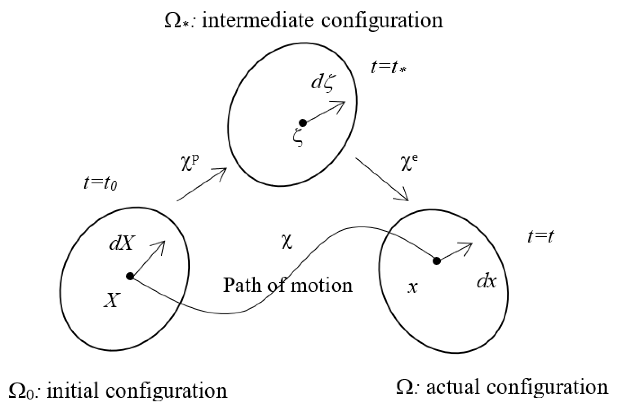
For rocks with elastoplastic deformation, we need to analyze three configurations. As shown in Figure 1 below, in the initial configuration Ω₀, the rock is undeformed, and X, the micro element at any point, is denoted as dX. The deformed rock is the current configuration Ω, which has undergone much plastic deformation. The micro element at any point, namely x of the deformed rock, is denoted as dx. In addition, the intermediate configuration Ω_* is also introduced. The intermediate configuration is assumed to be obtained from the initial configuration through pure plastic deformation or from the current configuration through the process of elastic unloading, where the micro element at any point ζ is denoted as dζ.

A point X on Ω₀ is mapped to a point ζ on the intermediate configuration Ω_* under the mapping χ^p:

$${\chi }^p:X\to \zeta$$

(1)

Due to the presence of these defects, the initial configuration is a material of manifold. In local coordinates, the neighborhood of point X has coordinates (X¹, …, X³); the neighborhood of point ζ has coordinates (ζ¹, …, ζⁿ); χ^p is a continuous mapping; and the transformation matrix between X and ζ is ∂ζ/∂X.

In differential geometry, χ^p is an immersion mapping of manifold M to manifold L, and the intermediate configuration is assumed to be a Riemannian manifold with a metric structure of a symmetric nonsingular covariant tensor field of the second order. In an analysis of local properties, it can be considered that M is embedded in L, inducing the push from the tangent space:

$${\chi }_{*}^p:{\eta }^I(X){\partial }_I\to {\eta }^I(X)A_I^{\alpha }{\partial }_{\alpha }={\overline{\eta }}^{\alpha }{\partial }_{\alpha }$$

(2)

A metric is defined in a Riemannian manifold as

$$d{s}_{*}^2=g_{\alpha \beta }d{\zeta }^{\alpha }d{\zeta }^{\beta }$$

(3)

The metric tensor field g_αβ on L is dragged back to the metric field G_IJ on M by

$$d{s}_{*}^2=g_{\alpha \beta }{A}_I^{\alpha }{A}_J^{\beta }d{X}^{I}d{X}^J=G_{IJ}d{X}^{I}d{X}^J$$

(4)

The metric tensor g of manifold L is determined by the distribution of rock defects and the degree of plastic deformation, while the metric tensor G of manifold M is determined by the distribution of these rock defects.

The element dX at a point X in the initial configuration can be related to the element dζ at a point ζ in the intermediate configuration through nonholonomic transformation:

$$d\zeta =AdX$$

(5)

A is the nonholonomic coefficient. The components satisfy

$$d{\zeta }^{\alpha }=A_I^{\alpha }d{X}^I,e_{\alpha }=A_I^{\alpha }{e}_I$$

(6)

Point ζ on Ω_* is mapped to point x on Ω under mapping χ^e:

$${\chi }^e:\zeta \to x$$

(7)

There is a tangent mapping at ζ:

$${\psi }_{*}:T_{\zeta }({\Omega }_{*})\to T_x(\Omega )$$

(8)

The local coordinate of point ζ is (ζ¹, …, ζⁿ), the corresponding coordinate of point x is (x¹, …, x³), χ^e is a continuous mapping, and the transformation matrix between ζ and x is ∂x/∂ζ. The metric tensor of the current configuration N is determined by the metric tensor G of the intermediate configuration and the elastic deformation ε^e.

Because the elastic deformation is reversible, we have

$$dx=Fd\zeta$$

(9)

F is the deformation gradient, and its components satisfy

$$d{x}^i=F_{\alpha }^{i}d{\zeta }^{\alpha },e_i=F_i^{\alpha }{e}_{\alpha }$$

(10)

The deformation of rocks can be considered as occurrences in a three-dimensional Euclidean space in a small range. The total deformation from the initial configuration to the current configuration is

$$\chi ={\chi }^e·{\chi }^p$$

(11)

Since the rock is in a three-dimensional Euclidean space before and after the deformation, the total deformation is compatible, so χ is bijective, and according to the composite mapping theorem, if χ_p is injective, then χ_e is surjective.

The initial configuration is in a three-dimensional Euclidean space, and the length square of the element at point X is

$$d{s}_0^2={\delta }_{IJ}d{X}_I{X}_J$$

(12)

The intermediate configuration is a Riemannian manifold, whose element length squared is

$$d{s}_{*}^2=g_{\alpha \beta }d{\zeta }^{\alpha }d{\zeta }^{\beta }=g_{\alpha \beta }{A}_I^{\alpha }{A}_J^{\beta }d{X}^{I}d{X}^J$$

(13)

The current configuration is also in a three-dimensional Euclidean space, and its element length squared is

$$d{s}^2={\delta }_{ij}d{x}^{i}d{x}^j={\delta }_{ij}{F}_I^i{F}_J^{j}d{X}^{I}d{X}^J=F_I^K{F}_J^{K}d{X}^{I}d{X}^J$$

(14)

Therefore, the change in the squared length of the element from the intermediate configuration to the current configuration is

$$d{s}^2-d{s}_{*}^2=(F_I^K{F}_J^K-g_{IJ})d{X}^{I}d{X}^J=2{\epsilon }_{IJ}^{e}d{X}^{I}d{X}^J$$

(15)

where ${\epsilon }_{IJ}^e$ is the elastic strain tensor. If we substitute the displacement equation into Equation (15), we will have

$$\begin{array}{l}{\epsilon }_{IJ}^e=\frac{1}{2}(F_I^K{F}_J^K-g_{IJ})=\frac{1}{2}[({\delta }_{kI}+\frac{\partial u_k}{\partial x_I})({\delta }_{kI}+\frac{\partial u_k}{\partial x_J})-g_{IJ}]\\ =\frac{1}{2}[{\delta }_{IJ}+\frac{\partial u_I}{\partial x_J}+\frac{\partial u_J}{\partial x_I}+\frac{\partial u_k}{\partial x_I}\frac{\partial u_k}{\partial x_J}-g_{IJ}]\\ =\frac{1}{2}(\frac{\partial u_I}{\partial x_J}+\frac{\partial u_J}{\partial x_I}+\frac{\partial u_k}{\partial x_I}\frac{\partial u_k}{\partial x_J})+\frac{1}{2}({\delta }_{IJ}-g_{IJ})\end{array}$$

(16)

where ε_IJ is the strain tensor in classic elasticity strain. When the deformation of the rock is small, the quadratic term in the above equation can be ignored, i.e.,

$${\epsilon }_{IJ}^e={\epsilon }_{IJ}+\frac{1}{2}({\delta }_{IJ}-g_{IJ})$$

(17)

The last two terms of Equation (17) are incompatible deformation terms—that is, the existence of plastic deformation makes the elastic deformation itself uncoordinated. Generally, the local coordinate basis {E_I} of the initial configuration is different from the local coordinate basis {e_i} of the current configuration. When the incremental deformation is small, the same coordinate basis vector {E_I} = {e_i} can be selected. Then, the above equation can be written as

$${\epsilon }_{ij}^e={\epsilon }_{ij}+\frac{1}{2}{\delta }_{ij}-\frac{1}{2}{g}_{ij}$$

(18)

3. Stress-Strain Relationship of the Incompatible Plastic Deformation

In the present section, we consider a Stress-Strain relationship of the incompatible plastic deformation. A number of variables and symbols are listed as follows:

• The total strain tensor ε_ij;
• The elastic strain tensor ${\epsilon }_{ij}^e$;
• The plastic strain tensor ${\epsilon }_{ij}^p$;
• The internal metric tensor g_ij;
• The elastic stiffness tensor C_ijkl;
• The elastic stress tensor ${\sigma }_{ij}$;
• The plastic multiplier dλ;
• The plastic potential w;
• The yield function F;
• The flow vector a;
• The hardening parameter κ;
• The usual matrix of elastic constants D;
• The incompatible parameter R;
• The elastic-plastic stiffness matrix Dep;
• The three principal stresses σ₁, σ₂, σ₃;
• The three principal deviatoric stresses ${\sigma }_1^{\prime }$, ${\sigma }_2^{\prime }$, ${\sigma }_3^{\prime }$;
• The three stress invariants J₁, J₂, J₃;
• The three invariants of deviatoric stress $J_1^{\prime }$, $J_2^{\prime }$, $J_3^{\prime }$;
• The internal friction angle ϕ;
• The cohesion c.

After the rock enters the state of plastic deformation, the strain at any point is composed of elastic strain and plastic strain. When the external load has a small increment, the total strain also has a small increment. The total strain increment consists of an elastic strain increment and a plastic strain increment, namely

$$d{\epsilon }_{ij}=d{\epsilon }_{ij}^e+d{\epsilon }_{ij}^p$$

(19)

By substituting Equation (18) into Equation (19), we will obtain

$$d{\epsilon }_{ij}^e=d{\epsilon }_{ij}+\frac{1}{2}d{\delta }_{ij}-\frac{1}{2}d{g}_{ij}-d{\epsilon }_{ij}^p=d{\epsilon }_{ij}-\frac{1}{2}d{g}_{ij}-d{\epsilon }_{ij}^p$$

(20)

The relationship between the elastic stress increment and strain increment can be determined by Hooke’s law as

$$d{\sigma }_{ij}=C_{ijkl}d{\epsilon }_{kl}^e$$

(21)

where C_ijkl is the elastic stiffness tensor. Since the plastic strain can be obtained through the flow law, the Stress-Strain relationship for ideal elastoplastic materials can be expressed as

$$d{\sigma }_{ij}=C_{ijkl}\left(d{\epsilon }_{ij}-d\lambda \frac{\partial w}{\partial {\sigma }_{kl}}-\frac{1}{2}d{g}_{kl}\right)$$

(22)

where dλ is an undetermined nonnegative scalar termed the plastic multiplier. During the plastic deformation, the stress point stays on the yield surface, and this supplementary condition is called the consistency condition, which is expressed by the following formula as

$$dF=\frac{\partial F}{\partial \sigma }d\sigma +\frac{\partial F}{\partial \kappa }d\kappa =a^{T}d\sigma -Ad\lambda =0$$

(23)

with the definitions of

$$a^T=\frac{\partial F}{\partial \sigma }=\left[\frac{\partial F}{\partial {\sigma }_x},\frac{\partial F}{\partial {\sigma }_y},\frac{\partial F}{\partial {\sigma }_z},\frac{\partial F}{\partial {\tau }_{yz}},\frac{\partial F}{\partial {\tau }_{zx}},\frac{\partial F}{\partial {\tau }_{xy}}\right]$$

(24)

$$A=-\frac{1}{d\lambda }\frac{\partial F}{\partial \kappa }d\kappa$$

(25)

The vector a is termed the flow vector. Equation (22) can be immediately rewritten as

$$(1-R)d\epsilon ={[D]}^{-1}d\sigma +d\lambda \frac{\partial F}{\partial \sigma }$$

(26)

where D is the usual matrix of elastic constants. Setting dg_kl/dε_kl = 2 R, according to Equation (18), we can obtain

$$R=\frac{d{g}_{kl}}{d{\epsilon }_{kl}}=1-\frac{d{\epsilon }_{kl}^e}{d{\epsilon }_{kl}}=1-\frac{E}{E_e}$$

(27)

where E_e is the elastic modulus of an intact rock, and E is the elastic modulus of a rock with defects. The parameter R reflects the influence of microscopic defects on macroscopic deformation of the rock.

Premultiplying both sides of Equation (26) by using $d_D^T=a^{T}D$ and eliminating a^Tdσ by the use of Equation (23), we can obtain

$$d\lambda =\frac{(1-R)}{A+a^{T}Da}{a}^T{d}_{D}d\epsilon$$

(28)

Substituting Equation (28) into Equation (26) we can obtain the complete incompatible elastic-plastic incremental Stress-Strain relation as

$$d\sigma =D_{ep}d\epsilon$$

(29)

where

$$D_{ep}=(1-R)(D-\frac{d_D{d}_D^T}{A+d^{T}a});d_D=Da$$

(30)

For numerical computation, it is convenient to write the yield function in terms of stress invariants. The advantage is that it permits the computer coding of yield function and the flow rule in a general form [17]. The principal deviatoric stresses ${\sigma }_1^{\prime }$, ${\sigma }_2^{\prime }$, ${\sigma }_3^{\prime }$ are given as the roots of the cubic equation [18]

$$t^3-J_2^{\prime }t-J_3^{\prime }=0$$

(31)

Noting the trigonometric identity

$${\sin }^3\theta -\frac{3}{4}\sin \theta +\frac{1}{4}\sin 3\theta =0$$

(32)

and setting t = rsinθ and substituting into Equation (31), we can obtain

$${\sin }^3\theta -\frac{J_2^{\prime }}{r^2}\sin \theta -\frac{J_3^{\prime }}{r^3}=0$$

(33)

Comparing Equation (32) and Equation (33), we can obtain

$$r=\frac{2}{\sqrt{3}}{(J_2^{\prime })}^{\frac{1}{2}}$$

(34)

$$\sin 3\theta =-\frac{J_3^{\prime }}{r^3}=-\frac{3\sqrt{3}}{2}\frac{J_3^{\prime }}{{(J_2^{\prime })}^{3/2}}$$

(35)

By noting the cyclic nature of sin (θ + 2 nπ), we have immediately made the three possible values of sinθ which define the three principal stresses. The deviatoric principal stresses are given by t = rsinθ upon substitution of the three values of sinθ in turn. Substituting for r from Equation (34) and adding the mean hydrostatic stress component give the total principal stresses as

$$\left\{\begin{array}{l}{\sigma }_1\\ {\sigma }_2\\ {\sigma }_3\end{array}\right\}=\frac{2}{\sqrt{3}}{(J_2^{\prime })}^{\frac{1}{2}}\left\{\begin{array}{l}\sin (\theta +\frac{2\pi }{3})\\ \sin \theta \\ \sin (\theta +\frac{4}{3}\pi )\end{array}\right\}+\frac{J_1}{3}\left\{\begin{array}{l}1\\ 1\\ 1\end{array}\right\}$$

(36)

with σ₁ > σ₂ > σ₃. For geomaterials, they typically have a frictional strength and different strengths in tension and in compression, so we can choose the Mohr–Coulomb yield criterion and write it in terms of J₁, J₂, and θ as

$$\frac{1}{3}{J}_1\sin \varphi +{(J_2^{\prime })}^{\frac{1}{2}}(\cos \theta -\frac{1}{\sqrt{3}}\sin \theta \sin \varphi )=c\cos \varphi$$

(37)

In order to calculate the D_ep matrix in (30), we need to express vector a in a form suitable for numerical computation as

$$a^T=\frac{\partial F}{\partial \sigma }=\frac{\partial F}{\partial J_2}\frac{\partial J_2}{\partial \sigma }+\frac{\partial F}{\partial {\left(J_2^{\prime }\right)}^{1/2}}\frac{\partial {\left(J_2^{\prime }\right)}^{1/2}}{\partial \sigma }+\frac{\partial F}{\partial \theta }\frac{\partial \theta }{\partial \sigma }$$

(38)

Differentiating Equation (35), we can obtain

$$\frac{\partial \theta }{\partial \sigma }=\frac{-\sqrt{3}}{2\cos 3\theta }\left[\frac{1}{{\left(J_2^{\prime }\right)}^{3/2}}\frac{\partial J_3}{\partial \sigma }-\frac{\partial J_3}{{\left(J_2^{\prime }\right)}^2}\frac{{\left(J_2^{\prime }\right)}^{1/2}}{\partial \sigma }\right]$$

(39)

Substituting Equation (38) in Equation (37) and using Equation (35), we can write a as

$$a=C_1{a}_1+C_2{a}_2+C_3{a}_3$$

(40)

where

$$a_1^T=\frac{\partial J_1}{\partial \sigma }=\{1,1,1,0,0,0\}$$

(41)

$$a_2^T=\frac{\partial {\left(J_2^{\prime }\right)}^{1/2}}{\partial \sigma }=\frac{1}{2{\left(J_2^{\prime }\right)}^{1/2}}\left\{s_x,s_y,s_z,2{\tau }_{yz},2{\tau }_{zx},2{\tau }_{xy}\right\}$$

(42)

$$a_3^T=\frac{\partial J_3}{\partial \sigma }=\left\{\begin{array}{l}(s_y{s}_z-{\tau }_{yz}^2+\frac{J_2^{\prime }}{3}),(s_x{s}_z-{\tau }_{xz}^2+\frac{J_2^{\prime }}{3}),(s_x{s}_y-{\tau }_{xy}^2+\frac{J_2^{\prime }}{3}),\\ 2({\tau }_{zx}{\tau }_{xy}-s_x{\tau }_{yz}),2({\tau }_{yz}{\tau }_{xy}-s_y{\tau }_{zx}),2({\tau }_{yz}{\tau }_{zx}-s_z{\tau }_{xy})\end{array}\right\}$$

(43)

and

$$C_1=\frac{\partial F}{\partial J_1}$$

(44)

$$C_2=\frac{\partial F}{\partial {(J_2^{\prime })}^{1/2}}-\frac{\tan 3\theta }{{(J_2^{\prime })}^{1/2}}\frac{\partial F}{\partial \theta }$$

(45)

$$C_3=\frac{-\sqrt{3}}{2\cos 3\theta }\frac{1}{{(J_2^{\prime })}^{3/2}}\frac{\partial F}{\partial \theta }$$

(46)

The C₁, C₂, and C₃ are the constants related to the yield surface. The tunnel excavated in underground engineering can be regarded as a problem of two-dimensional plane strain. According to the Mohr-Coulomb yield criterion, the equation from Equation (40) to Equation (46) can be written as

$$a_1^T=\{1,1,0,1\}$$

(47)

$$a_2^T=\frac{1}{2{\left(J_2^{\prime }\right)}^{1/2}}\left\{s_x,s_y,2{\tau }_{xy},s_z\right\}$$

(48)

$$a_3^T=\frac{\partial J_3}{\partial \sigma }=\left\{(s_y{s}_z+\frac{J_2^{\prime }}{3}),(s_x{s}_z+\frac{J_2^{\prime }}{3}),2s_z{\tau }_{xy},(s_x{s}_y+\frac{J_2^{\prime }}{3}),\right\}$$

(49)

and

$$C_1=\frac{1}{3}\sin \varphi$$

(50)

$$C_2=\cos \theta \left[\left(1+\tan \theta \tan 3\theta \right)+\sin \varphi \left(\tan 3\theta -\tan \theta \right)/\sqrt{3}\right]$$

(51)

$$C_3=\frac{\sqrt{3}\sin \theta +\cos \theta \sin \varphi }{2J_2^{\prime }\cos 3\theta }$$

(52)

4. Numerical Analysis

The FORTRAN language was used to write the elastic-plastic finite element program for the problem of two-dimensional plane strain. The parameters are listed as follows. It is assumed that the rock satisfies the associated flow rule, which is the Mohr–Coulomb yield criterion: the material constants include a Young’s modulus E = 21 GPa, a Poisson’s ratio v = 0.3, an internal friction angle ϕ = 30°, and a cohesion c = 5.85 MPa. The problem chosen is a thick-walled cylinder subjected to the external pressure P, with plane strain conditions assumed in the axial direction. Axisymmetry normally only requires analyzing a segment of the cylinder. For example, a 90° segment (see Figure 2) is used here to take advantage of the symmetry conditions along the x and y axes.

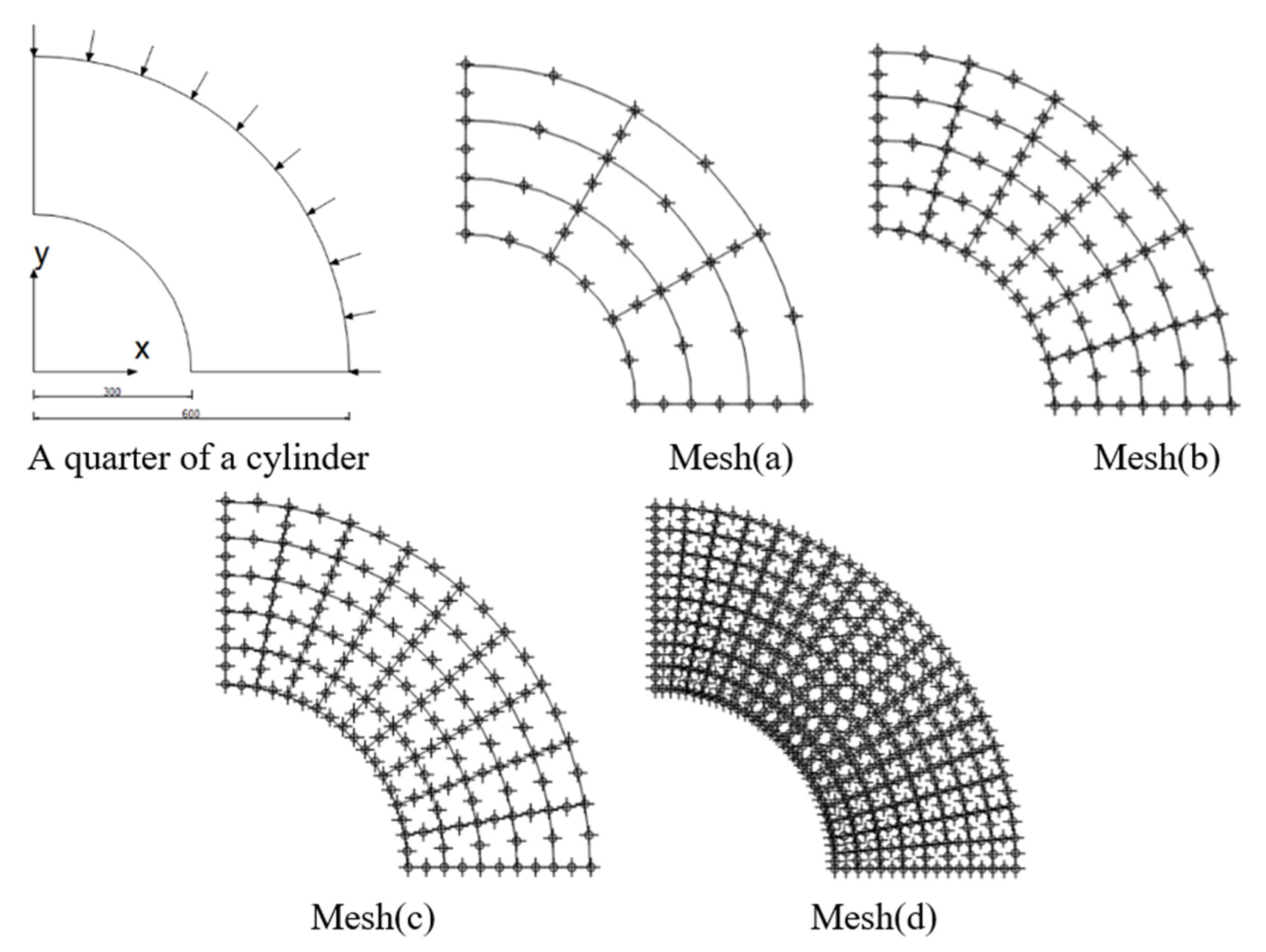
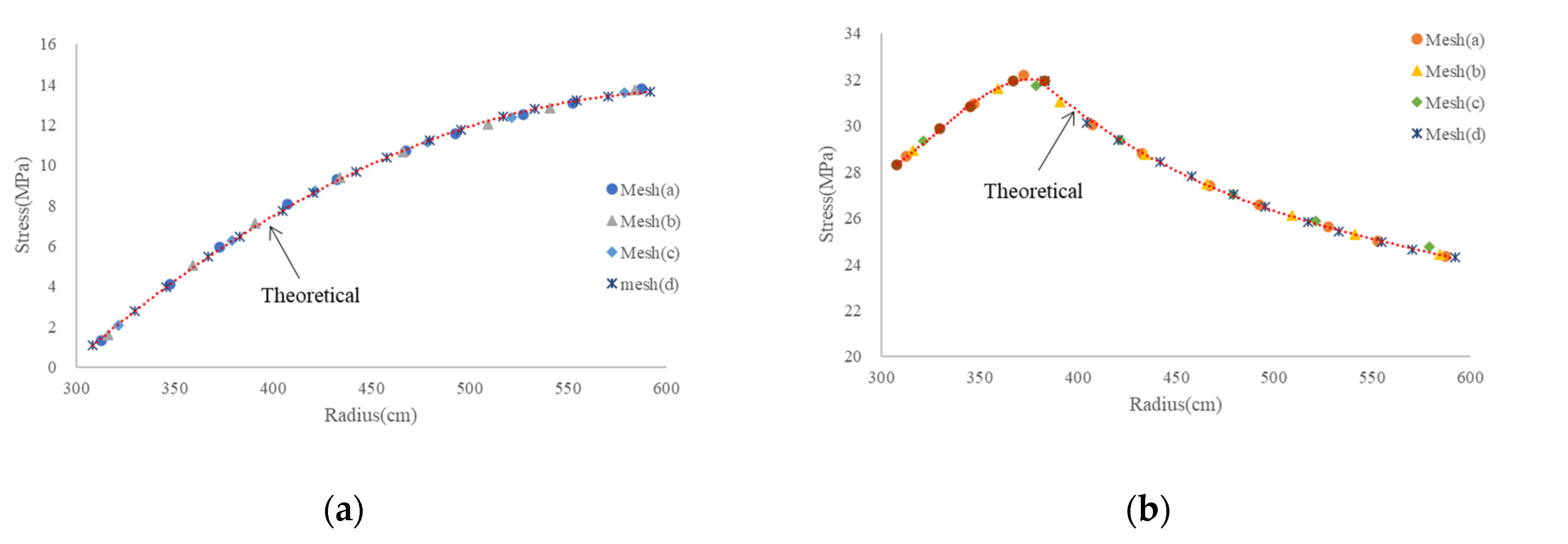
Before analyzing the problem, a sensitivity analysis of mesh is necessary. A number of different mesh divisions are shown in Figure 2, where an eight-node quadrangle element was chosen.

Referring to Figure 3, it can be seen that the results of meshes are quite reasonable since the results of radial stress and tangential stress are coincident with the results in the theoretical curve.

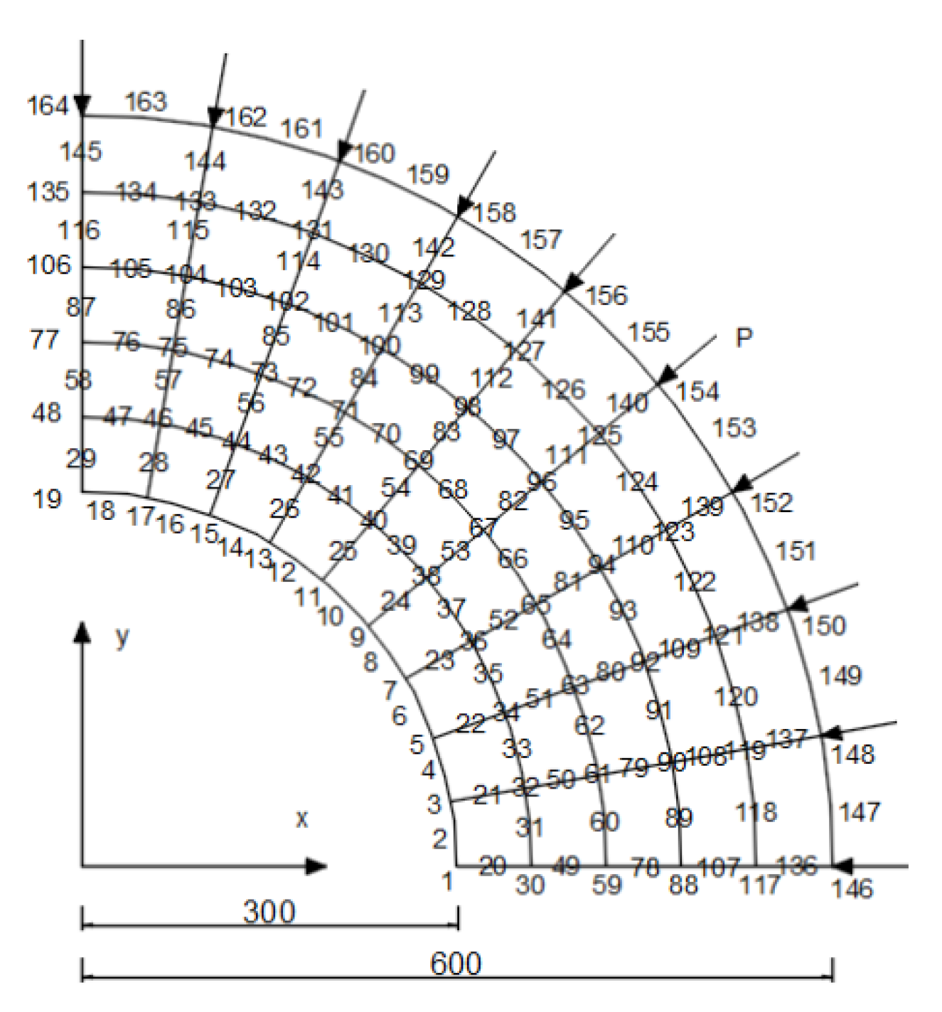
Thus, mesh(c) will be used because of the higher accuracy and relatively small amount of computation involved. After having decided on the element type and mesh division, it is now possible to prepare the data before putting them into the program. Such data are extracted directly from the drawing of the structure (see Figure 4) in which all information concerns nodes and element numbers, and load and boundary conditions are available.

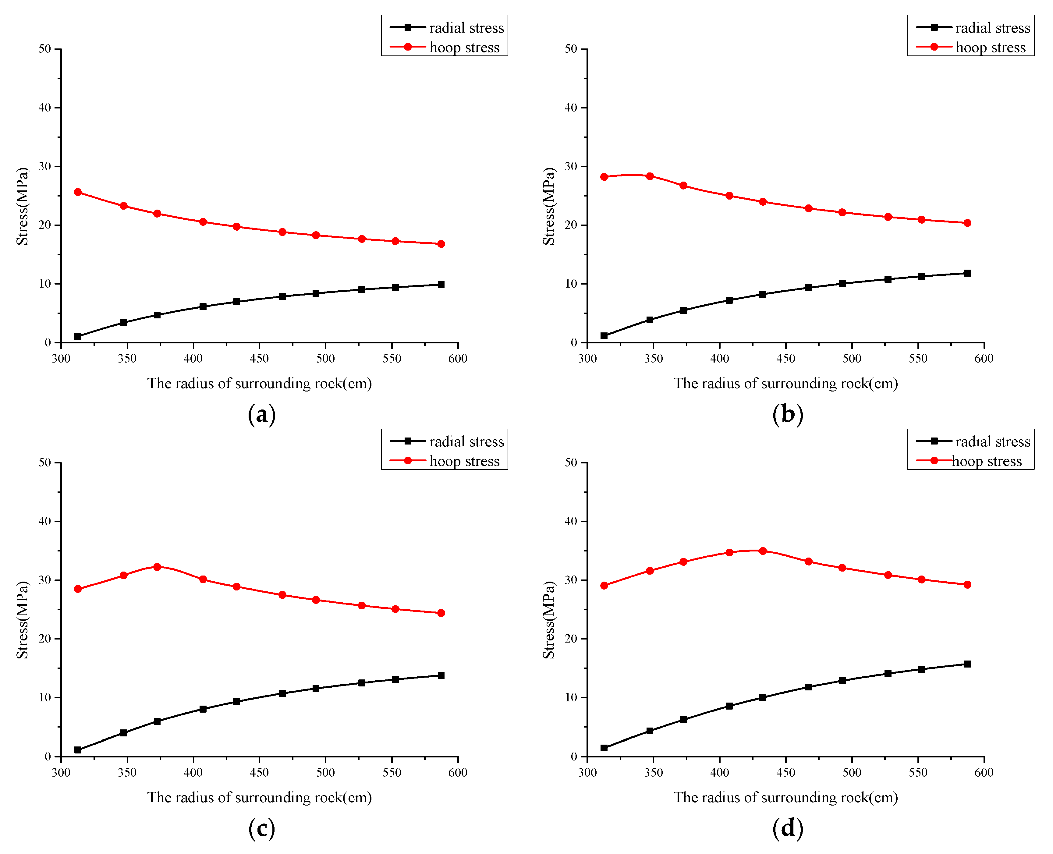
When the surrounding rock is intact, or with no defects, the distribution of stress is shown in Figure 5 below. When the pressure level of the surrounding rock is at 10 MPa, the surrounding rock is in an elastic state, and the distribution of hoop stress and radial stress is completely consistent with the elastic solution. With the increase in the surrounding rock stress, when the pressure of the surrounding rock is at 12 MPa, the plastic state appears 0.5 m closer to the inside of the tunnel, and the hoop stress increases first and decreases with the radius. The rock to the left of the peak point is in a plastic state, while the rock to the right of the peak point is in an elastic state. As the pressure of the surrounding rock continues to increase (14 MPa, 16 MPa, 18 MPa), the plastic zone of the surrounding rock also expands, and the radius of the plastic zone can be 3.35 m, 4.25 m, and 5.25 m. When the pressure of the surrounding rock reaches 19.4 MPa, all rocks in the region come to a plastic state.

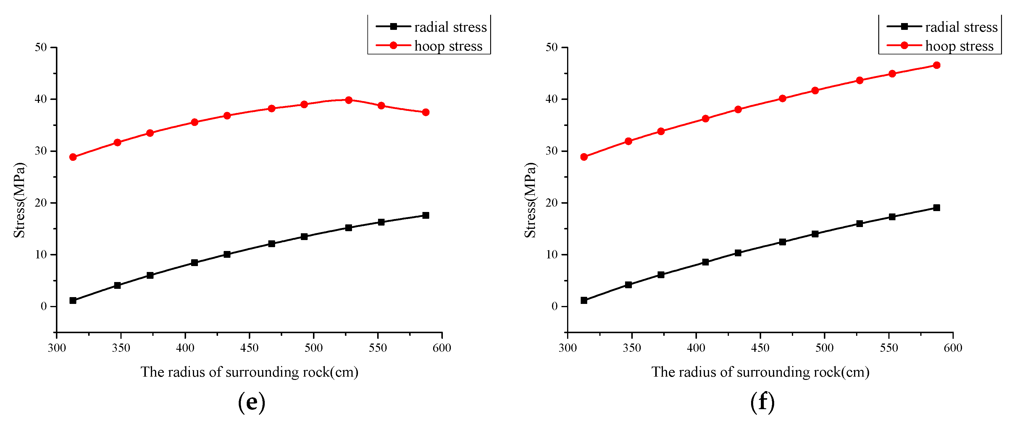
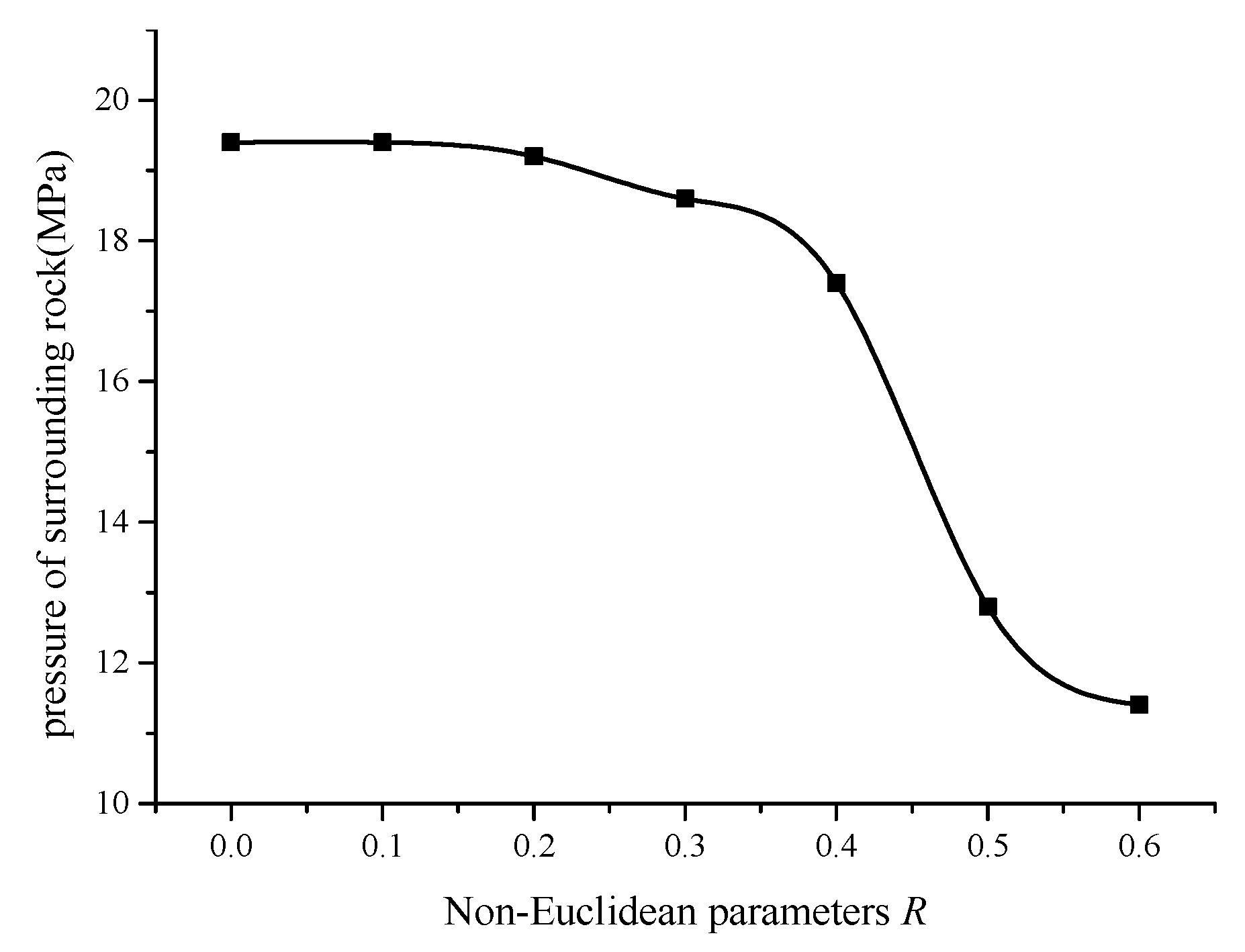
When the surrounding rock is a defect mass, the stiffness of the surrounding rock decreases due to the existence of the defect, per se, and the changes are shown in Figure 6 below. When R = 0, the rock has no defects, and the surrounding rock reaches a plastic state at 19.4 MPa. When R = 0.2, the surrounding rock reaches the plastic state at 19.2 MPa, indicating that the existence of defects reduces the stiffness of the surrounding rock, but the defects have little influence on the stress of the surrounding rock. When R = 0.4, the surrounding rock reaches a plastic state at 17.4 MPa, and the influence of the defects of the surrounding rock stress is further increased. When R = 0.5, the defects have a significant effect on the surrounding rock, and the surrounding rock reaches plasticity at 12.8 MPa.

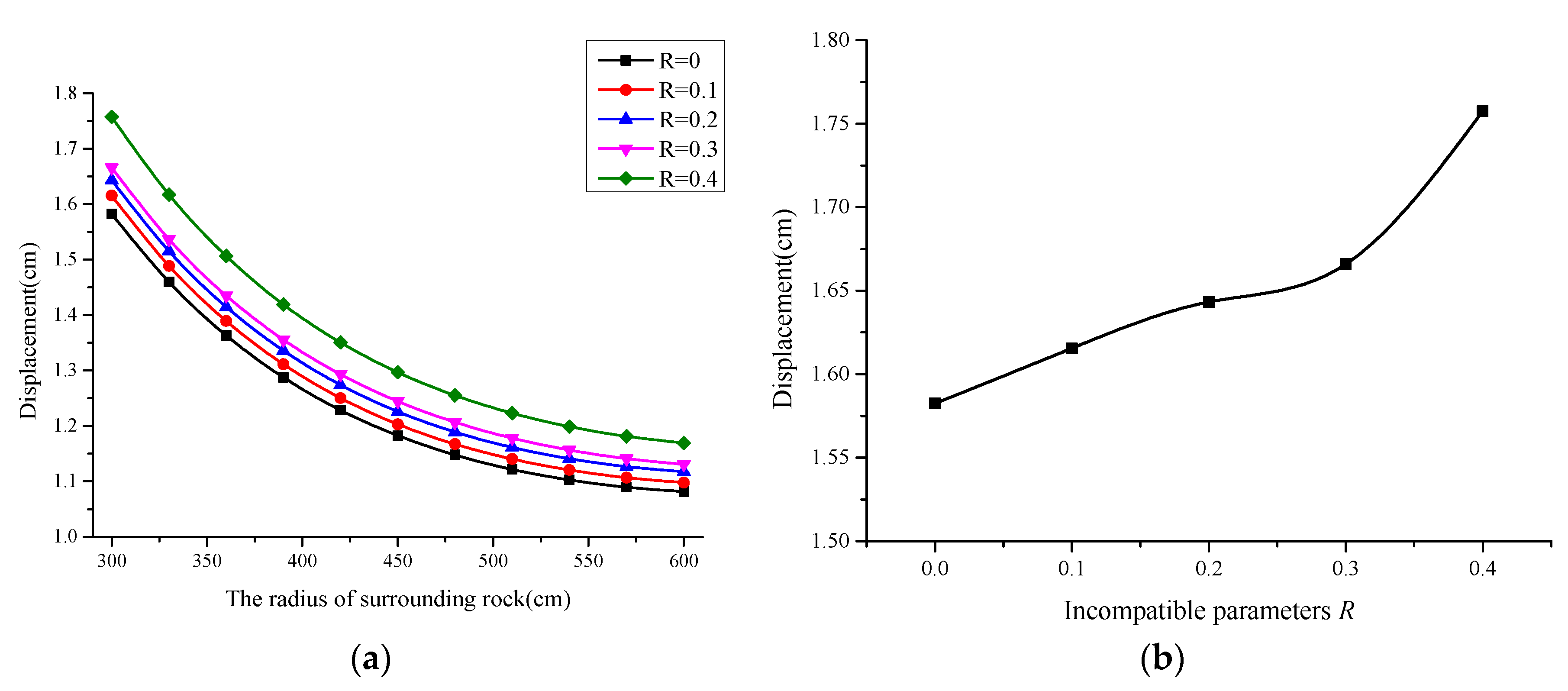
Due to the existence of defects, the stiffness of the surrounding rock decreases, and the deformation increases. The variation rule of deformation with incompatible parameters when the stress of the surrounding rock is at 19 MPa is assessed, as shown in Figure 7 below. When R increases from 0.1 to 0.3, the displacement of the surrounding rock increases linearly; when R reaches 0.4, the displacement increases more greatly than what it was before.

5. Conclusions

(1)

The existence of defects is the cause of incompatible deformation, and plastic deformation is the result of incompatible deformation as well. Although the deformed object has undergone much plastic deformation, it still exists in a three-dimensional Euclidean space, so the rock before and after the deformation is in a Euler space. The incompatible plastic deformation leads to the incompatible elastic deformation, while the total deformation can be coordinated.

(2)

When the deformation of the rock is small, the deformed and undeformed body can use the same coordinate base vector, and assuming the rock is an ideal plastic material, we can obtain the incremental plastic Stress-Strain relationship of the rock. The plastic strain increment is not only associated with the deviatoric stress state but also with the defect distribution. This distribution can be expressed as an incompatible parameter R. The larger the value of R is, the more defects there are in the rock and the smaller the elastic-plastic stiffness matrix will be.

(3)

The excavation of a deep underground tunnel can be regarded as a problem of two-dimensional plane strain. An elastic-plastic finite element program is written in the FORTRAN language to analyze circular tunnels under hydrostatic pressure. As the existence of defects decreases the stiffness of the surrounding rock, the larger the value of parameter R is, the faster the rock enters the plastic state and the larger the deformation of the surrounding rock will be.