1. Introduction
Simulation of soil yield processes is often computationally expensive, especially when analysing active clays such as MX-80 bentonite [
1], FEBEX bentonite [
2], or GMZ bentonite [
3]. These materials, which usually have a high smectite content, when hydrated unconfined from partially saturated conditions, can undergo deformations of 500%. Under confined conditions, they can lead to swelling pressures approaching 10 MPa. This makes the simulation of their hydromechanical behaviour always computationally demanding, particularly when simulating complex domains or when simulations have to be repeated a large number of times. Even considering the development experienced in recent years by microelectronic technology, which has allowed the multi-core and many-core hybrid heterogeneous parallel computing platform to facilitate a very important advance in computing power, the efficiency of the calculation algorithm continues to be a key issue in the application of massive calculation processes. This is shown, for example, in [
4] where the application of the Generalized Likelihood Uncertainty Estimation method in the probabilistic estimation of parameters in hydrology is analysed. In the field of soil mechanics, the improvement of computational performance is especially important in design or parameter identification processes, where the computational time can determine the viability of the study [
5].
In some constitutive models, such as the critical state soil models, both the stress space [
6] and the plastic terms
Dp of the elastoplastic matrix
Dep [
7,
8,
9] can be normalized. Thus, different stress states are associated with the same point of the normalized yield surface and with the same
Dp. The result could be that when solving boundary value problems, for a nonnegligible number of times, the calculations associated with the plastic behaviour of the same point (or in the vicinity of the same point) of the normalized stress space are repeated. It is therefore interesting to precompute
Dp for a grid of normalised stresses and to interpolate any value within the points of that grid when solving boundary value problems.
This approach is the resolution strategy proposed in the present work. In the following sections, the normalisation of the yield surface and Dp is first described. Then, the CPU time savings that the precomputation entails are evaluated. Later, the criteria are defined to ensure that the proposed method does not compromise the quality of the simulation, and finally, an inspection exercise is performed to evaluate its performance in solving boundary problems.
2. Theoretical Background
In addition to saturated conditions, this paper also assumes axisymmetric conditions. These hypotheses do not reduce the scope of the proposed formulation and yet allow it to be explained more clearly. Furthermore, in line with this quest for clarity, the modified Cam Clay model (MCCm) [
6] is adopted as the reference critical state soil model. In this way, the complexity of the constitutive formulation is reduced to a minimum, and the present work is focused on the description of the proposed calculation method. However, the widespread use of the MCCm in computational geotechnics [
10,
11,
12] means that the methodology presented here is not trivial.
Usually, the yield surface
f of the MCCm is formulated as
where
q is the von Mises deviatoric stress,
M is the slope of the critical state line, and the isotropic preconsolidation pressure
pO is the hardening parameter. This parameter is a good normalisation parameter since by introducing the dimensionless stresses
P =
p/
pO and
Q =
q/
pO,
f projects onto
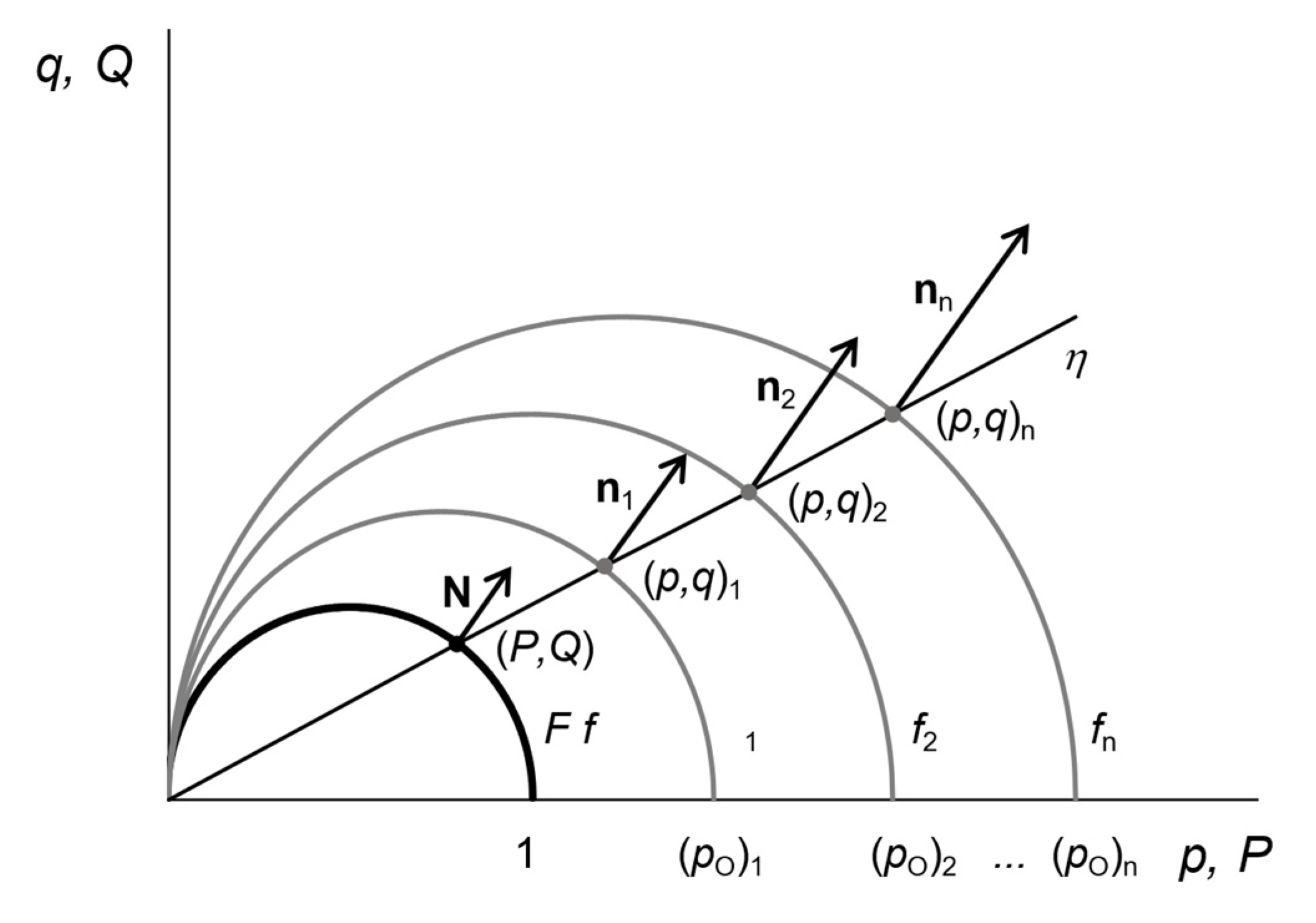
F (
Figure 1), as defined by the expression
All the points (
p,
q)
i located on the same axis
η, although they are associated with a different hardening parameters
pOi, define the same dimensionless stress (
P,
Q) (
Figure 1). Moreover, in all of them, the vector
n, normal to
f, given by the expression
has the same direction of
N, with its modulus varying according to the
pO factor. Therefore, assuming an associated plasticity model, the plastic terms of the elastoplastic matrix will be the same for all yield stresses which project onto the same dimensionless stress. Indeed, if the elastoplastic matrix
Dep defines the increase in the effective stress
dσ associated with an increase in the strain
dε (the Voigt notation is used for both stress and strain tensors), then we have
If the consistency equation is applied to the definition of the yield surface
f and both the flow rule and the hardening law are considered, then
Dep can be expressed as (see, for example, [
13,
14])
where
De is the elastic strain matrix,
I is the identity matrix with the dimension of
De, the symbol (·)
t indicates the transpose operator, and
x defines the vector of hardening parameters. As noted, in the MCCm,
x is equal to the scalar
pO. Its value is usually defined in critical state models by the hardening law
where
λ is the slope of the virgin compression line of the soil, and
dεVp is the volumetric plastic strain. For the axisymmetric conditions adopted, where
dε = (
dεV,
dε S) in which
dε S is the deviatoric strain,
Dp can be calculated as
where
fν is a function of Poisson’s ratio given by
Dividing by (
pO)
2 results in the dimensionless expression
Additionally,
De is defined as
where
K is the bulk modulus
and
G is the shear modulus
These moduli depend on the void ratio and are updated as the soil is loaded and deformed. Therefore, the elastic stiffness matrix depends on the strain path followed, as well as the preconsolidation stress, which must be updated according to Equation (6) from the volumetric plastic strain. However, Equation (9) shows that
Dp depends on
P and
Q only. Actually, it depends on only one parameter, since both
P and
Q are on the surface
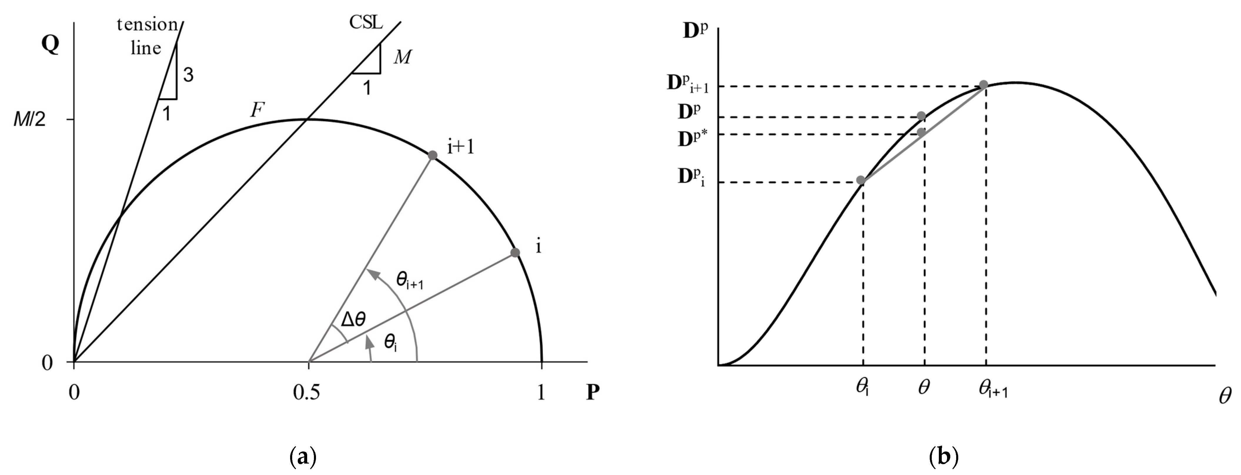
F = 0 (
Figure 1), which, like
Dp, can be parametrised by the angle
θ shown in
Figure 2. Furthermore, in this figure, it is proposed to select
N equispaced points (with an Δ
θ angle between them) at
F = 0, calculating
Dpi for each of them. Subsequently, when solving a boundary value problem, the value of
Dp is approximated by the interpolation
Dp* for angle values between two previously calculated values
obtaining
Dep* by
The calculation procedure proposed in this work is based on precomputing the vector of matrices {Dp1, Dp2, …, DpN}, thus avoiding repeating the calculation of Dp during the resolution of the boundary value problems.
3. Evaluation of the Precomputation Efficiency
The efficiency of the proposed procedure depends on the cost of calculating
Dp. If this cost is not an important part of the total cost of the calculation process, the performance associated with using
Dp* might not be of interest.
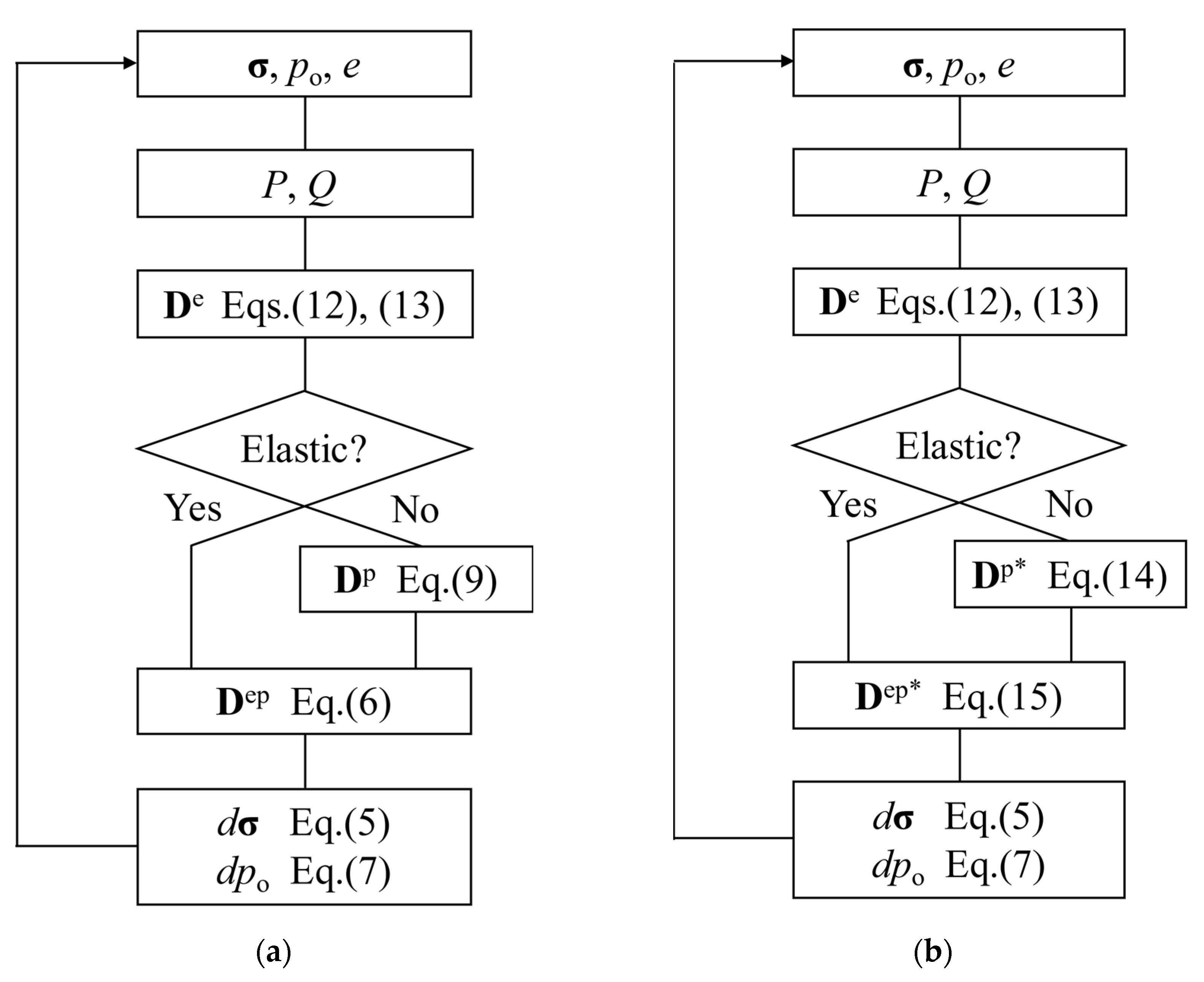
Figure 3a summarises the process followed to solve a computational step when integrating the constitutive model.
Table 1 lists the number of operations associated with the calculation of
De and
Dp. Although these numbers can vary depending on the way in which the algorithm is programmed, the changes are not significant in terms of the relative computational cost of each magnitude. Using the results of the benchmark defined in
Appendix A (where it is indicated that the estimated cost of each multiplication is equivalent to 1.101 sums, with the cost of division being 3.698 sums), the costs shown in the last column of
Table 1 were obtained. While it is advisable to be cautious about the reliability in absolute terms of the representativeness of these numbers, they do characterise the weight that each calculation carries in relative terms.
Figure 3b shows the strategy followed when applying the precomputational procedure. As noted,
De must be calculated as in the conventional method. In addition, interpolation of the
Dpi matrices must be made to obtain
Dp* by performing the operations indicated in
Table 1. Using again the values of
Appendix A, the computational cost of
Table 1 is obtained, which is approximately 42% of the cost of calculating
Dp. The computational time savings are remarkable, and the application of the approach proposed here is therefore of interest.
4. Precomputation Density
To define the precomputation strategy, the minimum number of points N to be taken at
F = 0 must be determined in such a way that the accuracy of the calculation when using
Dp* is comparable to the accuracy obtained when calculating
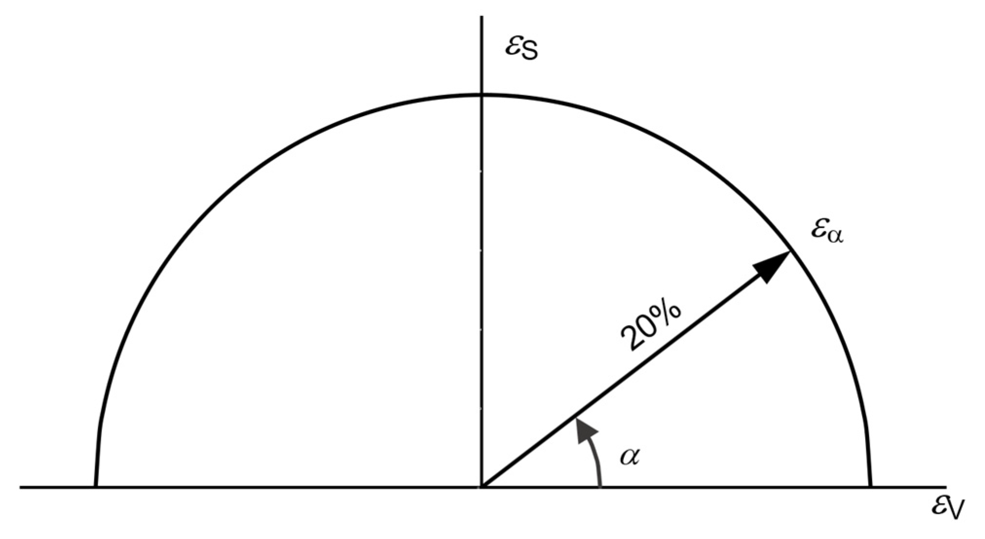
Dp. To accomplish this goal, a set of constant strain rate paths with a final strain of 20% and with different ratios between volumetric and shear strains, as in
Figure 4, were inspected. In all of these inspection exercises, initial spherical conditions were assumed with an effective mean stress of
p =
pO/2 = 200 kPa. The analysis was performed for the three soils, namely Weald clay, Klein Belt Ton, and kaolin, which are characterised in
Table 2. The differences between their properties make the conclusions reached not limited to a particular material.
As a reference, all paths were simulated using an explicit Euler integration method. An intensive substepping process was applied, i.e., the number of calculation steps was divided into smaller substeps successively until the solution differed from the previous solution by only the sixth significant digit, which is a strategy similar to that used by Sołowski and Gallipoli [
16]. These results were compared with the precomputed–interpolated solution using the same number of substeps during the explicit integration.
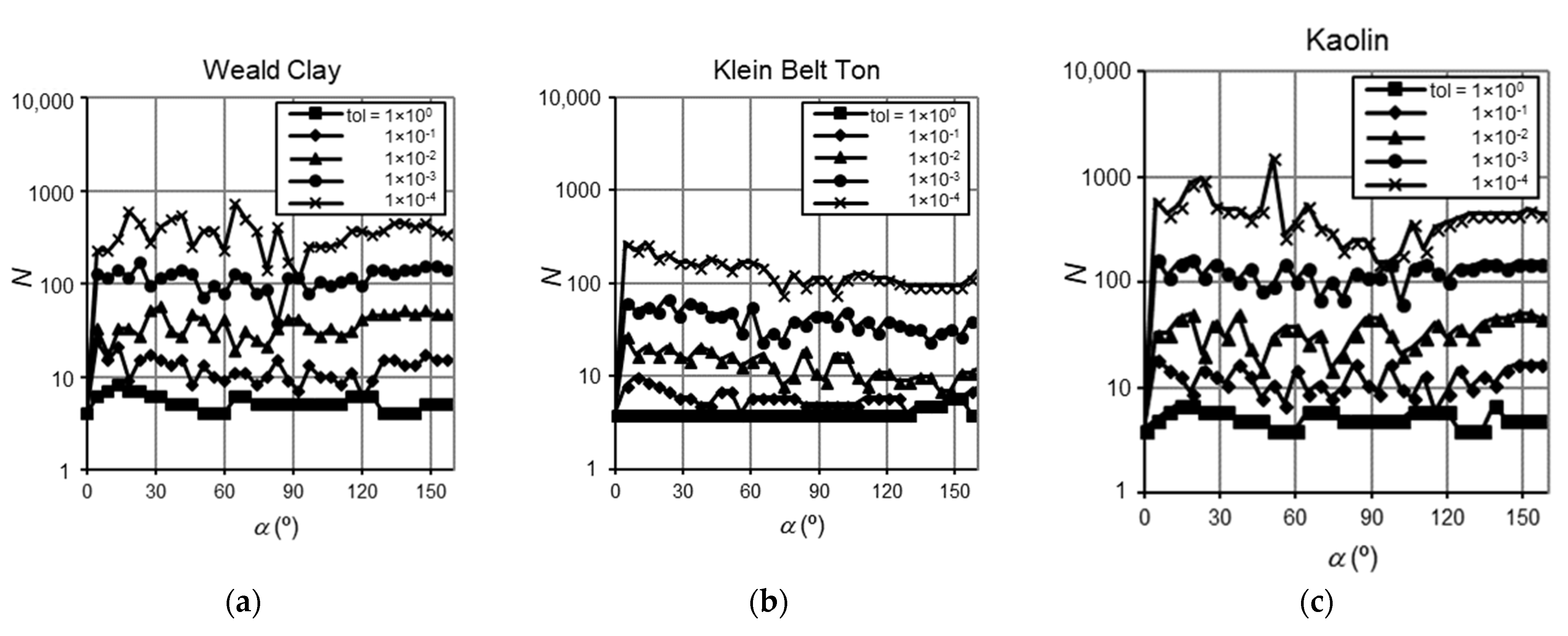
For each path, for each value of
α in
Figure 4, the number of points N to be computed on the yield surface was determined in such a way that the normalised root-mean-square deviation between the stress solution obtained by explicit Euler integration and the solution reached by calculation with the precomputation–interpolation procedure was less than 10
0, 10
−1, 10
−2, 10
−3, and 10
−4.
Figure 5 shows the values of N obtained for each of these tolerances and for each value of
α.
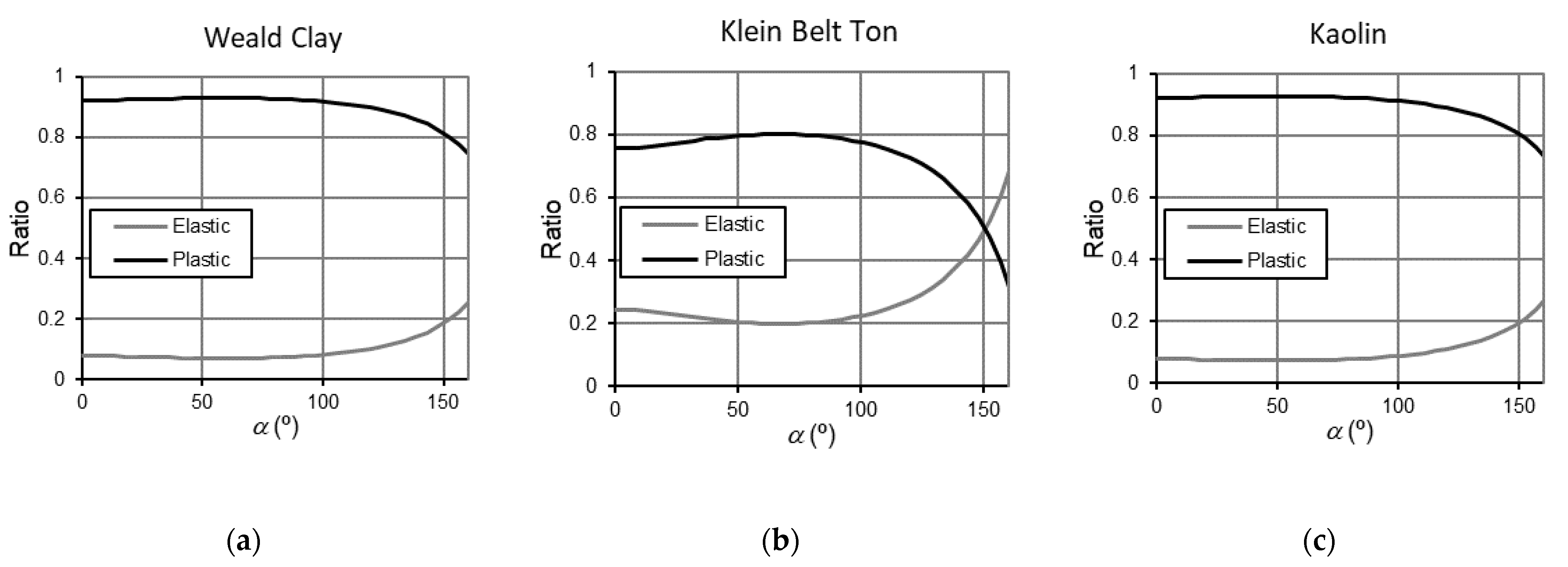
It is important to note that, as illustrated in
Figure 6, when imposing a total strain of 20%, in all cases, a significant yield was attained. In other words, trajectories that were highly sensitive to the quality of the precomputation results were analysed.
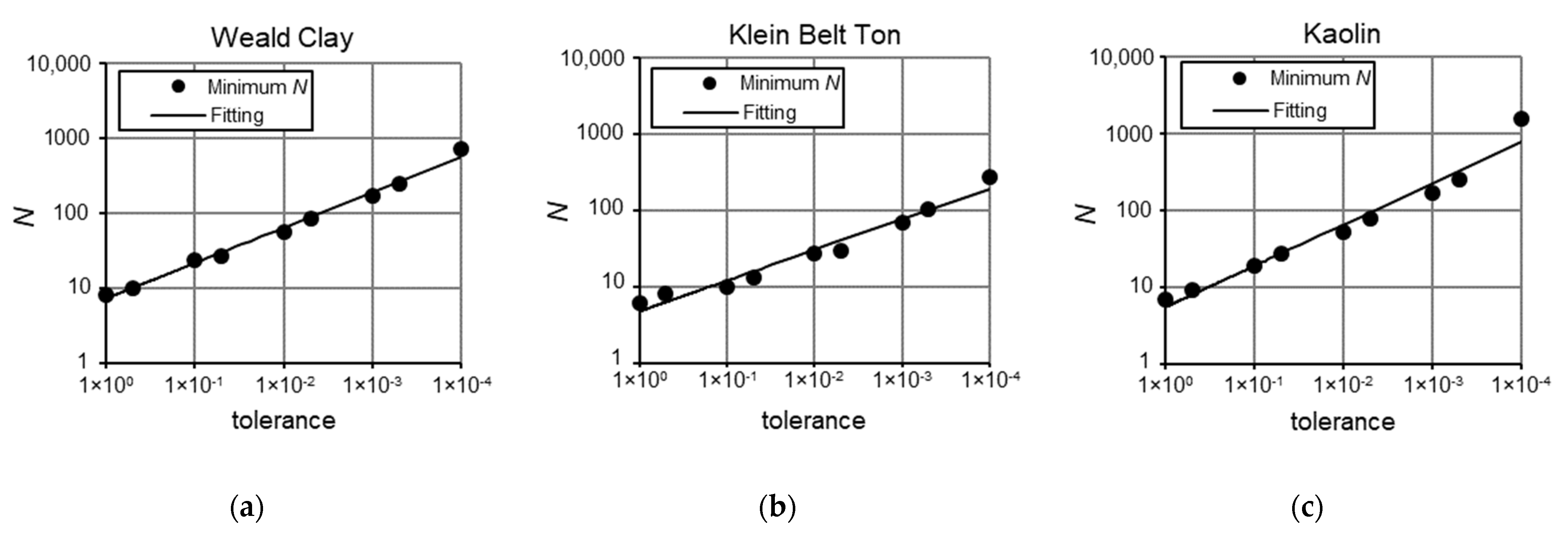
In all paths, as the tolerance decreased, N increased. This trend can be clearly seen in
Figure 7, where for each tolerance value, the maximum value of N obtained for any
α was plotted. The behaviour of N was well defined and not erratic; additionally,
Figure 7 can be used to define the number of points N to be taken to avoid exceeding a certain value of tolerance.
5. An Inspection on Solving Boundary Value Problems
Although the comparison in
Table 1 highlights the interest of the precomputational approach, it does not illustrate its scope clearly enough, because it is associated with the simulation of individual stress–strain paths. Considering a finite element model in which conventionally the stresses are a state function, those paths would illustrate the behaviour of a single Gaussian point. It is reasonable to question what will happen when, in a real problem, the number of Gaussian points is in the hundreds or thousands.
It is not easy to answer this question. Savings will depend on the structure of the finite element code used and the calculation and information management strategies implemented. Each code will have a different response. However, in general, it is reasonable to assume that if
NGP is the number of Gaussian points considered in the mesh, the cost of a conventional explicit integration,
χC, can be estimated as
where the computational costs of
De and
Dp, and
CDe and
CDp have been defined (as well as the computational cost of
Dp* and
CDp*) in
Table 1, and for the total number of computational time steps needed to solve the boundary problem,
ηΔεe defines the weighted value of the elastic increments, and
ηΔεep defines one of the elastoplastic increments. In turn, the cost of the precomputation–interpolation strategy,
χPI, is estimated as
where
ηΔεe* and
ηΔεep* are the values analogous to
ηΔεe and
ηΔεep, respectively, when the integration of the constitutive model is done using the precomputation and interpolation procedure. Their values can, in principle, be different. However, since the discretization of the yield surface is proposed with a very demanding tolerance (10
−4 in the analyses performed above), it is to be expected that
ηΔεe* ≈
ηΔεe and
ηΔεep* ≈
ηΔεep. In this case,
ρ, the ratio between the cost of a traditional explicit integration and the cost of the precomputation–interpolation strategy, is given by the expression
The relative cost is independent of the mesh size. Furthermore, it is necessary to add to the computational costs considered in Equations (15) and (16) the costs associated with the generation of the database {
Dp1,
Dp2, …,
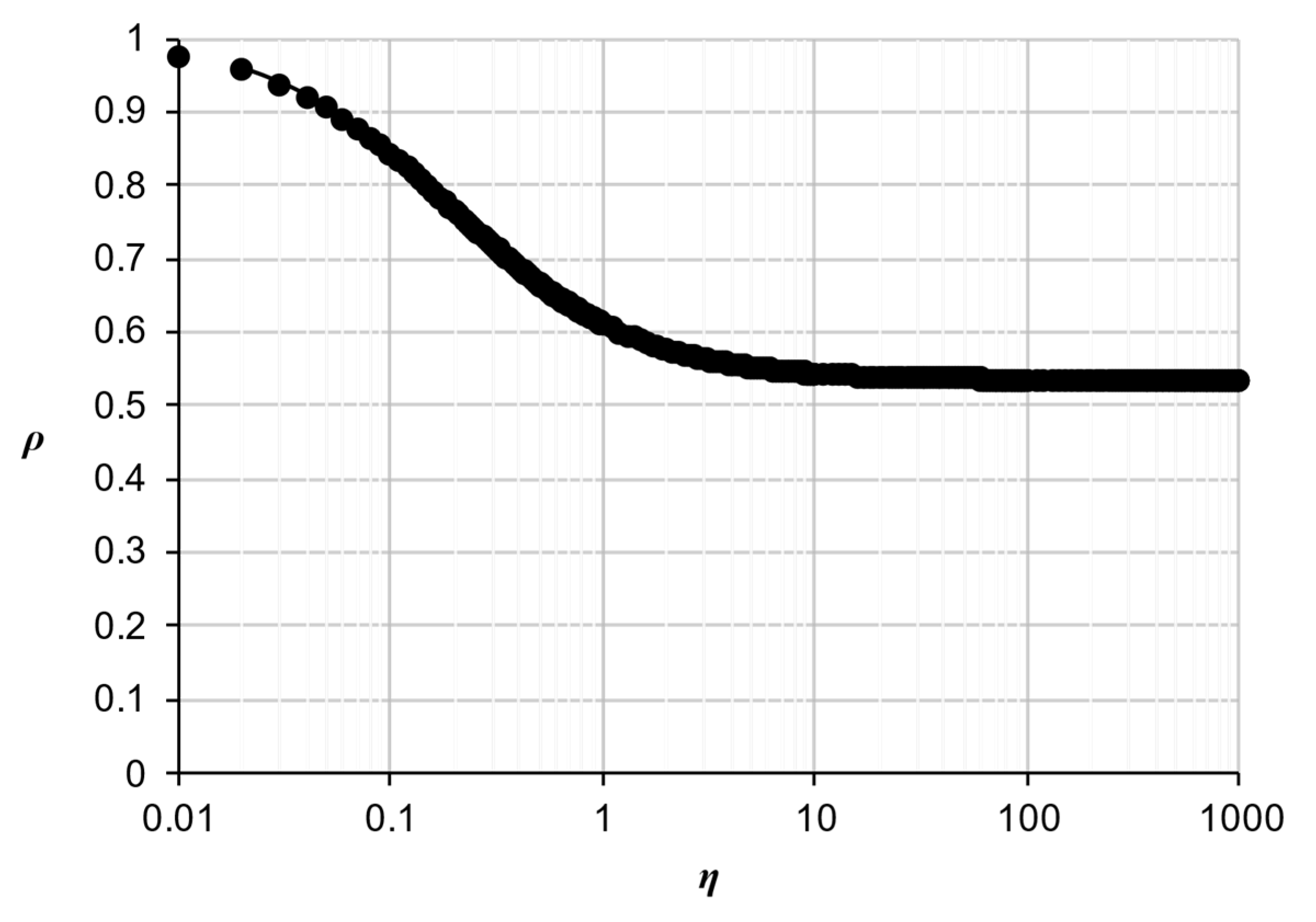
DpN}. Consequently, it is to be expected that if the mesh is small, the relative importance of the precomputation cost is not negligible. However, the proposed methodology is oriented to large-scale computation, and thus it is a consistent estimator of the efficiency, and for a large computational volume, as shown in Equation (17), it is independent of the mesh size. The ratio
η =
ηΔεep/
ηΔεe expresses the relative importance of the computation of plastic steps in a problem. As expected, given that the precomputation is aimed at optimizing the calculation of the plastic steps, its efficiency is conditioned by the relevance of the plastic strains over the elastic strains, in other words, by the value of
η. Using the values of
CDe,
CDp, and
CDp* from
Table 1, the change in
ρ with respect to
η was plotted and is shown in
Figure 8. If
η = 0, when the yield is not reached, precomputation is not applied. Only elastic steps are calculated, and both methods are equal (
ρ = 1). However, as seen at the end of
Section 3, as soon as some plastic steps are required, the precomputation is more efficient (
ρ < 1). The larger the volume of the calculation of the plastic steps, the higher the efficiency. When the entire calculation is in the plastic regime (i.e., in normally consolidated conditions), the efficiency tends to a maximum value of 54%.


 ,
, 