Reliability Study of Parameter Uncertainty Based on Time-Varying Failure Rates with an Application to Subsea Oil and Gas Production Emergency Shutdown Systems

Abstract

The failure rate of equipment during long-term operation in severe environment is time-varying. Most studies regard the failure rate as a constant, ignoring the reliability evaluation error caused by the constant. While studying failure data that are few and easily missing, it is common to focus only on the uncertainty of reliability index rather than parameter of failure rate. In this study, a new time-varying failure rate model containing time-varying scale factor is established, and a statistical-fuzzy model of failure rate cumulated parameter is established by using statistical and fuzzy knowledge, which is used to modify the time-varying failure rate model. Subsequently, the theorem of the upper boundary existence for the failure rate region is proposed and proved to provide the failure rate cumulated parameter when the failure rate changes the fastest. The proposed model and theorem are applied to analyze the reliability of subsea emergency shutdown system in the marine environment for a long time. The comparison of system reliability under time-varying failure rate and constant failure rate shows that the time-varying failure rate model can eliminate the evaluation error and is consistent with engineering. The reliability intervals based on the failure rate model before and after modification are compared to analyze differences in uncertainty, which confirm that the modified model is more accurate and more practical for engineering.

1. Introduction

As the core part of subsea production system, subsea control system has important functions of monitoring production status and manipulating control equipment [1,2,3]. The mainstream type of subsea control system is multiplexed electro-hydraulic control system, which has short response time, high redundancy and low cost of umbilical cable, and can give consideration to both reliability and economy [4,5,6]. An indispensable part of the multiplexed electro-hydraulic control system is subsea emergency shutdown (ESD) system, which can prevent the occurrence of major production accidents to a great extent, ensure the stable production of oil and gas fields, and protect the personal safety of field personnel, production facilities, and marine environment [7]. Therefore, the reliability level of subsea ESD system determines the safe operation of offshore oil and gas exploitation, and its reliability evaluation is of far-reaching significance.

The failure rate of equipment during reliability evaluation is the essential data support. In most reliability studies, the failure rate of each equipment is usually simplified to a constant value due to the lack of basic data such as failure records of partial equipment. Wang et al. [8] established a reliability model for the electrical control system of the subsea control module by markov processes and multiple beta factor model using the constant failure rate (CFR) and its value range. When assessing the reliability and safety of subsea Christmas tree, Pang et al. [9] converted the failure rate of hydraulic and electronic components which obey an exponential distribution and mechanical components with Weibull distribution into a constant. Bae et al. [10] referred to the CFR of equipment in offshore and onshore reliability data (OREDA), and used the multi-objective design optimization method to optimize the ESD system to ensure its high reliability and reasonable cost. Signorini et al. [11] collected 106 subsea control module (SCM) field data sets and compared them with OREDA for quantitative and qualitative reliability study of SCM. None of these studies have considered the reliability evaluation error caused by the CFR. Not only is the field of offshore oil research prone to ignore this error, but numerous other fields tend to assume a CFR as well. Ismagilov et al. [12] proposed a combined method of analysis the reliability indicators based on functional-cost analysis and failure modes and effects analysis for the aviation electromechanical system, taking a CFR when calculating the failure occurrence probability. When calculating the reliability of the battery electric vehicle powertrain system, Tang et al. [13] simplified the failure rate into constant. Tawfiq et al. [14] used the block diagram technique to minimize the number of system component rates after integrating multiple factors, either failure or repair. It is considered that the failure rate unchanged during modeling.

The failure rate of the subsea ESD system varies over time after being affected by factors such as equipment, environment, and operation. Considering the time-varying characteristics of the equipment failure rate when establishing the reliability model, it can not only reduce the evaluation error caused by the CFR, but also deeply explore the impact of the time-varying failure rate (TFR) on reliability. Earlier Hassett et al. [15] used a general polynomial to express the TFR and proposed a hybrid reliability and availability analysis method combined with Markov chain analysis. In industrial applications, the failure rates of most equipment vary with the service life of components. Retterath et al. [16] established the TFR model of distribution system, then analyzed the impact of TFR on distribution system by Monte Carlo simulation. Wang et al. [17] divided the equipment failure of relay protection device into random failure and aging failure, and proposed the estimation approach for the TFR of relay protection device. Abunima et al. [18] determined the TFR of photovoltaic system by comprehensively considering weather conditions, PV system architecture and components, interactions of PV components with the weather conditions. Liu et al. [19] combined historical fault data with related weather forecasts to establish an overhead transmission line reliability model considering the TFR, thereby proposing an optimal inspection strategy. Zhang et al. [20] fitted the failure rate with the length of the submarine cables, and proposed an improved dynamic reliability model of the TFR based on the seasonal changes of the failure caused by fishing operations and anchor damage. Li et al. [21] established a multi-state Markov failure rate prediction model for transformers, and used the aging failure model to modify it to accurately predict the real-time failure rate. Liu et al. [22] used an exponential function that is more in line with the actual trend to characterize the TFR of the solenoid valve power supply, which accurately reflects the aging process of the power system. However, the parameter uncertainty of TFR model is not studied in this work.

The problem of parameter uncertainty is particularly prominent in reliability analysis, which brings uncertainty to the system reliability evaluation and affects the accuracy. When the reliability uncertainty exceeds a certain range, the result of reliability analysis will lose practical significance. Zhang et al. [23] discussed the influence of the uncertainty of each parameter on the output power performance, stability, and reliability by modeling the randomness of the parameters affecting the output of a photovoltaic cell. Li et al. [24] used non-sequential Monte Carlo simulation to establish the analytical expressions of variable reliability parameters, so as to establish a system of nonlinear equations for solving the reliability parameters of unknown equipment. Wang et al. [25] established the gray three-parameter Weibull distribution model of the relay protection device, and estimated the reliability parameters to ensure the calculation speed and accuracy. Miranda et al. [26] considered the uncertainty of stochastic equipment data in power system expansion planning, and calculated uncertainty by using interval arithmetic through the theory of imprecise probabilities. The parameters of the software reliability model were estimated and predicted by Zhen et al. [27] using the hybrid WPA-PSO algorithm. Wang et al. [28] carried out point estimation and approximate interval estimation of model parameters for Kijima type Weibull generalized renewal processes models I and II, and proposed a calculation method of the reliability indices for repairable systems with imperfect repair. The failure rates of the repairable system modules obeying exponential distribution were estimated by Uprety and Patrai [29] using the fuzzy triangle number obtained from the point estimation and confidence interval. Yang et al. [30] focused on the reliability uncertainty of wind power systems, and estimated the unknown parameters of the autoregressive integrated moving average prediction model using bayesian estimation methods based on Markov chain Monte Carlo. Wang et al. [31] utilized the statistical properties of the poisson binomial distribution to develop analytical confidence intervals for failure probability estimation. Hu et al. [32] regarded the state probability and performance rate of the multi-state device as uncertain variables, and combined with probability theory and uncertainty theory to introduce the uncertain universal generating function for reliability analysis of random uncertain multi-state system with missing samples. Li et al. [33] established a life model and uncertainty statistical method based on uncertainty theory considering life test type-I and type-II censoring, precise and interval data of failure data. Wang et al. [34] aimed at the uncertainty of the reliability data in the phasor measurement unit by combining statistical methods and fuzzy Markov to establish parameter membership functions of reliability indices, and evaluated the impact of parameter uncertainty. These studies only focus on system reliability indexes and ignore the uncertainty of failure rate parameters.

The failure rate of subsea emergency shutdown (ESD) system is time-varying due to long-term operation in complex marine environment, and its failure data has the characteristics of small quantity, long collection period, high confidentiality (less access). In order to solve the shortcomings that ignore the time-varying and simplify the failure rate to a constant value, ignore the existence of uncertainty in the failure rate parameter identified in previous studies, a new time-varying failure rate (TFR) model including time-varying scale factor is established in this study. Firstly, a statistical-fuzzy model of the failure rate cumulated parameter is established by combining statistical and fuzzy set knowledge, and the TFR model is effectively modified using this model. Secondly, for the modified TFR model, the theorem of upper boundary existence for failure rate region is proposed and proved. In this study, the above theoretical method is used for the subsea ESD system. By comparing and calculating the reliabilities of the systems under the TFR and CFR, it is shown that the new TFR model can eliminate the evaluation error caused by constant failure rate (CFR) and make the variation tendency of system reliability consistent with the industrial application. The upper boundary existence theorem accurately provides the failure rate cumulated parameter when the failure rate changes the fastest, and then uses TFR models before and after the modification to compare the uncertainty of failure rate cumulated parameter to the uncertainty of system reliability, the degrees of influence are different. The modified TFR model effectively corrects the reliability interval containing uncertainty.

The rest of this paper is organized as follows: in Section 2, the TFR model and the statistical-fuzzy model of failure rate cumulated parameter are established, and the TFR model is modified with the model of failure rate cumulated parameter. The theorem of upper boundary existence for the failure rate region is proposed and proved, and the numerical example is given in Section 3. Section 4 takes the subsea ESD system as the analysis object. Firstly, the reliabilities of the systems under the TFR and the CFR are compared and evaluated, and then the reliability simulations of the systems are compared and analyzed based on TFR models before and after modification. Finally, conclusions are given in Section 5.

2. Modeling and Modification

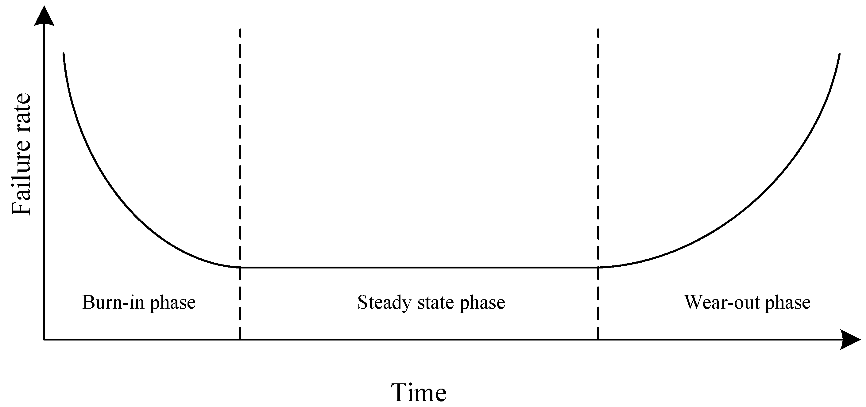
2.1. Time-Varying Failure Rate Model

Failure rate is one of the most important indexes for calculating reliability. Typical equipment failure rate is a curve with time of use as the abscissa and failure rate as the ordinate. Its trend is high at the beginning, low in the middle, and high at the end, so it is called the “bathtub curve” [35].

The bathtub curve is divided into burn-in phase, steady state phase, and wear-out phase, which is shown in Figure 1. Due to defects of equipment raw materials and manufacturing, the failure rate in the burn-in phase is usually high. Then the equipment operation after debugging and running-in tends to be normal, while the failure rate decreases. The failure rate of the steady state phase is constant and the lowest. Over time, the failure rate increases with the aggravation of equipment wear and fatigue, and enters the wear-out phase.

The equipment will complete factory acceptance tests to filter out early failures, so the TFR modeling can skip the burn-in phase and only consider the steady state phase and wear-out phase. The CFR in the steady state phase is usually used in reliability evaluation, that is, the exponential distribution which is too ideal for equipment is selected. Therefore, this study puts forward a time-varying scale factor and improves it in the wear-out phase to comprehensively describe the TFR in the steady state phase and wear-out phase.

The time-varying scale factor varies over time during the equipment life cycle, and the CFR is determined by the time-varying scale factor to increase or decrease. The TFR in this paper is as follows:

$$\lambda \left(t\right)=\epsilon \left(t\right){\lambda }_0,$$

(1)

where $\epsilon \left(t\right)$ is the time-varying scale factor and ${\lambda }_0$ is the CFR of the equipment. The time-varying scale factor of the steady state phase and the wear-out phase are given below, respectively.

• Steady state phase. The failure distribution is consistent with the bottom of the “bathtub curve” when the equipment is running normally, which means the failure rate is constant. The time-varying scale factor is a constant value of 1 in this phase.

  $$\epsilon \left(t\right)=1$$

  (2)
• Wear-out phase. The wear-out phase is usually described by Weibull distribution, because the shape parameter in Weibull distribution is excessive that will lead to a rapid rising trend of failure rate [22], the time-varying scale factor of the wear-out phase in this study adopts an exponential function to reasonably describe the rising trend of “bathtub curve”.

  $$\epsilon \left(t\right)=e^{\eta (t-T)},$$

  (3)

  where $\eta$ is the failure rate cumulated parameter of equipment, and T is the duration of the steady state phase. Combined with the previous equations, the TFR model of this paper is determined as:

  $$\lambda \left(t\right)=\epsilon \left(t\right){\lambda }_0=\left\{\begin{array}{cc}{\lambda }_0\hfill & t\le T\\ e^{\eta (t-T)}{\lambda }_0\hfill & t>T\end{array}\right.$$

  (4)

2.2. Statistical-Fuzzy Model of the Failure Rate Cumulated Parameter

There is a degree of uncertainty in the failure rate cumulated parameter obtained either by fitting failure data or by using expert experience. The fitting may suffer from missing data and low precision, and expert experience is subjective. In this paper, the interval value of the failure rate cumulated parameter is used instead of the single value, which can not only express the uncertainty of the parameter quantitatively, but also enable the reliability analysis result to cover this uncertainty. Since the concept of the cut set in fuzzy membership function is consistent with a range [34], this study uses the parameter estimation in mathematical statistics combined with expert experience to carry out interval estimation for failure rate cumulated parameter. The Pseudo-Gaussian (PG) membership function of the failure rate cumulated parameter is further obtained, and the statistical-fuzzy model of the failure rate cumulated parameter is established to directly reflect the uncertainty interval of the failure rate cumulated parameter.

The failure rate cumulated parameter $\eta$ is estimated using the chi-square distribution at a given significant level ${\alpha }_0$.

$$\left[{\eta }_L^{{\alpha }_0},{\eta }_U^{{\alpha }_0}\right]=\left[{\chi }_{1-{\alpha }_0/2}^2\left(2r\right)/2T_r,{\chi }_{{\alpha }_0/2}^2(2r+2)/2T_r\right](r=1,2,\cdots ,n-1),$$

(5)

$$\overline{\eta }={\eta }_0,$$

(6)

where ${\chi }_{1-{\alpha }_0/2}^2\left(2r\right)$ is the quantile when the integral from 0 to ${\chi }_{1-{\alpha }_0/2}^2\left(2r\right)$ of chi-square distribution is ${\alpha }_0/2$ under the degree of freedom $2r$, ${\chi }_{{\alpha }_0/2}^2(2r+2)$ is the quantile when the integral from ${\chi }_{{\alpha }_0/2}^2(2r+2)$ to ∞ is ${\alpha }_0/2$ under the degree of freedom $2r+2$. $T_r$ is the statistical time, and ${\eta }_0$ is the expert experience value.

Considering the asymmetry when using the chi-square distribution, a PG membership function of the failure rate cumulated parameter is established.

$$f(x,\sigma ,c)=\left\{\begin{array}{cc}exp\left[-\frac{{(x-c)}^2}{{{\sigma }_L}^2}\right]& x\le c\\ exp\left[-\frac{{(x-c)}^2}{{{\sigma }_R}^2}\right]& x>c\end{array}\right.,$$

(7)

where x represents the failure rate cumulated parameter, and c is the expert experience value of the failure rate cumulated parameter, ${\sigma }_L$ and ${\sigma }_R$ are the scale parameters of the left and right parts of the PG membership function, respectively.

The degree of membership is similar to the concept of significant level, both of which can reflect subjective confidence degree. Therefore, the upper and lower bounds of the failure rate cumulated parameter $\eta$ in (5) correspond to the upper and lower boundaries at the $1-{\alpha }_0$-cut of the PG membership function.

$$\left\{\begin{array}{c}exp\left[-\frac{{({\eta }_L^{{\alpha }_0}-{\eta }_0)}^2}{{{\sigma }_L}^2}\right]=1-{\alpha }_0\\ exp\left[-\frac{{({\eta }_U^{{\alpha }_0}-{\eta }_0)}^2}{{{\sigma }_R}^2}\right]=1-{\alpha }_0\end{array}\right.$$

(8)

${\sigma }_L$ and ${\sigma }_R$ of the PG membership function of $\eta$ can be estimated after the transformation of (8).

$$\left\{\begin{array}{c}{\sigma }_L=-({\eta }_L^{{\alpha }_0}-{\eta }_0)/\sqrt{-ln(1-{\alpha }_0)}\hfill \\ {\sigma }_R=({\eta }_U^{{\alpha }_0}-{\eta }_0)/\sqrt{-ln(1-{\alpha }_0)}\hfill \end{array}\right.$$

(9)

The PG membership function of the failure rate cumulated parameter can be obtained by substituting (9) into (7), which is a convex function in the real number field as shown in Figure 2.

Extending the PG membership function $f(\eta ,{\alpha }_i)$ to the general form as:

$$f(\eta ,{\alpha }_i)=\left\{\begin{array}{cc}exp\left[\frac{{(\eta -{\eta }_0)}^{2}ln(1-{\alpha }_i)}{{({\eta }_L^{{\alpha }_i}-{\eta }_0)}^2}\right]& \eta \le {\eta }_0\\ exp\left[\frac{{(\eta -{\eta }_0)}^{2}ln(1-{\alpha }_i)}{{({\eta }_U^{{\alpha }_i}-{\eta }_0)}^2}\right]& \eta >{\eta }_0\end{array}\right.,$$

(10)

where $1-{\alpha }_i$ is an arbitrary cut set.

2.3. Modification of Time-Varying Failure Rate Model

Different failure rate cumulated parameter $\eta$ corresponds to different trends of TFR curves, and the time-varying scaling factor characterizing by the exponential function increases monotonically with $\eta$ during wear-out phase, so $\left[{\eta }_L^{{\alpha }_i},{\eta }_U^{{\alpha }_i}\right]$ corresponds to a region enclosed by innumerable TFR curves. The upper and lower boundaries of the region are determined by the upper and lower boundaries of the interval, which intuitively reflects the degree of uncertainty contained in system reliability analysis. In order to make the reliability analysis of the system with uncertainty have practical significance, the uncertainty of the failure rate cumulated parameter cannot exceed a certain range, and the upper and lower boundaries of the region enclosed by the failure rate curves should be focused on. Considering that the membership function can be used to describe the degree to which the object belongs to a certain definition, this study proposes a new method to modify the TFR model by using the statistical-fuzzy model of the failure rate cumulated parameter. This method can more objectively and accurately specify the upper and lower boundaries of the region enclosed by the modified failure rate curves.

Firstly, the upper and lower boundaries of $\left[{\eta }_L^{{\alpha }_i},{\eta }_U^{{\alpha }_i}\right]$ and ${\eta }_0$ are substituted into (4), respectively, and the corresponding TFR models are as follows:

$${\lambda }_{{\eta }_L^{{\alpha }_i}}\left(t\right)={\epsilon }_{{\eta }_L^{{\alpha }_i}}\left(t\right){\lambda }_0=\left\{\begin{array}{cc}{\lambda }_0\hfill & t\le T\\ e^{{\eta }_L^{{\alpha }_i}(t-T)}{\lambda }_0\hfill & t>T\end{array}\right.$$

(11)

$${\lambda }_{{\eta }_U^{{\alpha }_i}}\left(t\right)={\epsilon }_{{\eta }_U^{{\alpha }_i}}\left(t\right){\lambda }_0=\left\{\begin{array}{cc}{\lambda }_0\hfill & t\le T\\ e^{{\eta }_U^{{\alpha }_i}(t-T)}{\lambda }_0\hfill & t>T\end{array}\right.$$

(12)

$${\lambda }_{{\eta }_0}\left(t\right)={\epsilon }_{{\eta }_0}\left(t\right){\lambda }_0=\left\{\begin{array}{cc}{\lambda }_0\hfill & t\le T\\ e^{{\eta }_0(t-T)}{\lambda }_0\hfill & t>T\end{array}\right.$$

(13)

The TFR curve drawn from (11)–(13) is shown in Figure 3. It can be directly observed that the failure rate curve corresponding to ${\eta }_L^{{\alpha }_i}$ rises the slowest, and the failure rate curve corresponding to ${\eta }_U^{{\alpha }_i}$ rises the most rapidly. The failure rate curve corresponding to ${\eta }_0$ is sandwiched between the upper and lower boundary curves. The failure rate ${\lambda }_{{\eta }_L^{{\alpha }_i}}<{\lambda }_{{\eta }_0}<{\lambda }_{{\eta }_U^{{\alpha }_i}}$ at any same time point in the wear-out phase.

To consider the confidence attached to $\eta$ in the failure rate model objectively, the TFR model is modified using the statistical-fuzzy model of $\eta$. This method is only for the wear-out phase where parameter uncertainty exists, and the modified model is as follows:

$${\lambda }_{mo}\left(t\right)=\lambda \left(t\right)·f(\eta ,{\alpha }_i)=e^{\eta (t-T)}{\lambda }_0·exp\left[\frac{{(\eta -{\eta }_0)}^{2}ln(1-{\alpha }_i)}{{({\eta }^{{\alpha }_i}-{\eta }_0)}^2}\right]$$

(14)

The upper and lower boundaries of $\left[{\eta }_L^{{\alpha }_i},{\eta }_U^{{\alpha }_i}\right]$ and ${\eta }_0$ are substituted into (14), and the corresponding modified TFR models are as follows:

$${\lambda }_{mo,{\eta }_L^{{\alpha }_i}}\left(t\right)=\left\{\begin{array}{cc}{\lambda }_0\hfill & t\le T\\ (1-{\alpha }_i)e^{{\eta }_L^{{\alpha }_i}(t-T)}{\lambda }_0\hfill & t>T\end{array}\right.$$

(15)

$${\lambda }_{mo,{\eta }_U^{{\alpha }_i}}\left(t\right)=\left\{\begin{array}{cc}{\lambda }_0\hfill & t\le T\\ (1-{\alpha }_i)e^{{\eta }_U^{{\alpha }_i}(t-T)}{\lambda }_0\hfill & t>T\end{array}\right.$$

(16)

$${\lambda }_{mo,{\eta }_0}\left(t\right)=\left\{\begin{array}{cc}{\lambda }_0\hfill & t\le T\\ e^{{\eta }_0(t-T)}{\lambda }_0\hfill & t>T\end{array}\right.$$

(17)

When the TFR model is modified by the statistical-fuzzy model of $\eta$, the size order of failure rates ${\lambda }_{{\eta }_L^{{\alpha }_i}}$, ${\lambda }_{{\eta }_0}$ and ${\lambda }_{{\eta }_U^{{\alpha }_i}}$ at any same time point in the wear-out phase will change, and the upper and lower boundaries of the region enclosed by TFR curves will also change synchronously. The degree of change is discussed in Section 3.

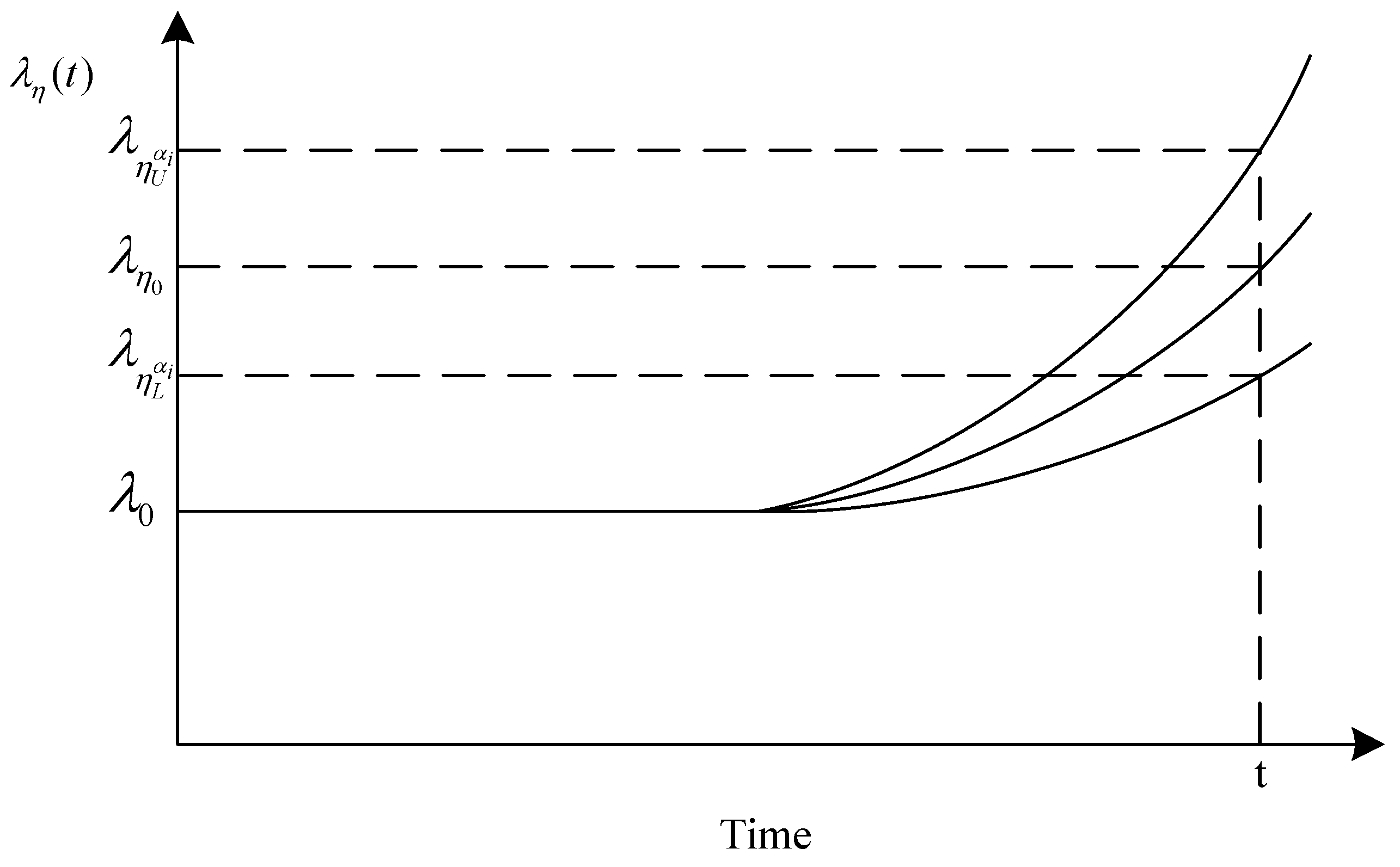
3. The Existence Proof of Upper Boundary of Modified TFR Region

3.1. The Upper Boundary Existence Theorem and Proof

The membership function of the failure rate cumulated parameter and the failure rate function of the wear-out phase both increase monotonically within the interval $\left[{\eta }_L^{{\alpha }_i},{\eta }_0\right]$. From (14), it can be seen that the modified failure rate function ${\lambda }_{mo,{\eta }_L^{{\alpha }_i}}\left(t\right)<{\lambda }_{mo,{\eta }_0}\left(t\right)$ always holds. Comparing (15) and (16), it can be seen that the modified failure rate function ${\lambda }_{mo,{\eta }_L^{{\alpha }_i}}\left(t\right)<{\lambda }_{mo,{\eta }_U^{{\alpha }_i}}\left(t\right)$ always holds. This study focuses on the TFR model modified by the PG membership function on the right half.

$${\lambda }_{mo}\left(t\right)=e^{\eta (t-T)}{\lambda }_0·exp\left[\frac{{(\eta -{\eta }_0)}^{2}ln(1-{\alpha }_i)}{{({\eta }_U^{{\alpha }_i}-{\eta }_0)}^2}\right]$$

(18)

The TFR function is shifted T units to the left ignoring the steady state phase, and the modified TFR model is simplified as:

$${\lambda }_{mo}\left(t\right)=e^{\eta t}{\lambda }_0·exp\left[\frac{{(\eta -{\eta }_0)}^{2}ln(1-{\alpha }_i)}{{({\eta }_U^{{\alpha }_i}-{\eta }_0)}^2}\right]$$

(19)

Theorem 1.

The upper boundary existence theorem.

Assuming that parameters t, ${\alpha }_i$, ${\eta }_0$, ${\lambda }_0$ are given, there is a definite upper boundary of the region bounded by ${\lambda }_{mo}\left(t\right)$ under the domain $\left[{\eta }_L^{{\alpha }_0},{\eta }_U^{{\alpha }_0}\right]$ of $\eta$, if and only if $\eta =min\left\{{\eta }_U^{{\alpha }_i},{\eta }_0-{({\eta }_U^{{\alpha }_i}-{\eta }_0)}^{2}t/2ln(1-{\alpha }_i)\right\}$.

Proof of Theorem 1. 

Given that t, ${\alpha }_i$, ${\eta }_0$, ${\lambda }_0$, so ${\eta }_U^{{\alpha }_i}$ is also a definite value, then only $\eta$ is the independent variable in ${\lambda }_{mo}\left(t\right)$. Rewrite ${\lambda }_{mo}\left(t\right)$ as ${\lambda }_{mo}\left(\eta \right)$, and take the derivative of $\eta$ in ${\lambda }_{mo}\left(\eta \right)$.

$$\frac{d{\lambda }_{mo}\left(\eta \right)}{d\eta }={\lambda }_0{e}^{\eta t}·exp\left[\frac{{(\eta -{\eta }_0)}^{2}ln(1-{\alpha }_i)}{{({\eta }_U^{{\alpha }_i}-{\eta }_0)}^2}\right]·\left[t+\frac{2(\eta -{\eta }_0)ln(1-{\alpha }_i)}{{({\eta }_U^{{\alpha }_i}-{\eta }_0)}^2}\right]$$

(20)

Let (20) be rewritten as:

$$\frac{d{\lambda }_{mo}\left(\eta \right)}{d\eta }=g\left(\eta \right)·h\left(\eta \right),$$

(21)

where:

$$g\left(\eta \right)={\lambda }_0{e}^{\eta t}·exp\left[\frac{{(\eta -{\eta }_0)}^{2}ln(1-{\alpha }_i)}{{({\eta }_U^{{\alpha }_i}-{\eta }_0)}^2}\right]$$

(22)

$$h\left(\eta \right)=t+\frac{2(\eta -{\eta }_0)ln(1-{\alpha }_i)}{{({\eta }_U^{{\alpha }_i}-{\eta }_0)}^2}$$

(23)

According to the properties of failure rate and the exponential function, ${\lambda }_0>0$, $e^{\eta t}>0$, $exp\left[\frac{{(\eta -{\eta }_0)}^{2}ln(1-{\alpha }_i)}{{({\eta }_U^{{\alpha }_i}-{\eta }_0)}^2}\right]>0$ always hold, therefore $g\left(\eta \right)>0$ always holds. The following focuses on $h\left(\eta \right)$.

$$h\left(\eta \right)=K\eta +R$$

(24)

Combining (23) and (24), the following can be obtained:

$$K=\frac{2ln(1-{\alpha }_i)}{{({\eta }_U^{{\alpha }_i}-{\eta }_0)}^2}$$

(25)

$$R=t-\frac{2{\eta }_{0}ln(1-{\alpha }_i)}{{({\eta }_U^{{\alpha }_i}-{\eta }_0)}^2}$$

(26)

${\alpha }_i\in \left[0,1\right]$, $t>0$, ${\eta }_0>0$ is known, so $K<0$, $R>0$ always hold. It can be seen that $h\left(\eta \right)$ is a straight line decreasing monotonically that intersects the positive vertical axis. Suppose the intersection point of $h\left(\eta \right)$ and the horizontal axis is ${\eta }^{\prime }$, it follows that ${\eta }^{\prime }>0$. Furthermore, it is known that:

$$\left\{\begin{array}{cc}h\left(\eta \right)>0& \eta <{\eta }^{\prime }\\ h\left(\eta \right)\le 0& \eta \ge {\eta }^{\prime }\end{array}\right.$$

(27)

Combining (21), (22), and (27) can be obtained:

$$\left\{\begin{array}{cc}\frac{d{\lambda }_{mo}\left(\eta \right)}{d\eta }>0& \eta <{\eta }^{\prime }\\ \frac{d{\lambda }_{mo}\left(\eta \right)}{d\eta }\le 0& \eta \ge {\eta }^{\prime }\end{array}\right.$$

(28)

Therefore, ${\lambda }_{mo}\left(\eta \right)$ increases first and then decreases progressively, and there must be a local maximum value in the real number field. Given $h\left({\eta }^{\prime }\right)=0$, the local maximum point is:

$${\eta }^{\prime }={\eta }_0-\frac{{({\eta }_U^{{\alpha }_i}-{\eta }_0)}^{2}t}{2ln(1-{\alpha }_i)}>{\eta }_0$$

(29)

Given $\eta \in \left[{\eta }_L^{{\alpha }_0},{\eta }_U^{{\alpha }_0}\right]$, to further obtain the maximum point of ${\lambda }_{mo}\left(\eta \right)$, compare the size of ${\eta }^{\prime }$ and ${\eta }_U^{{\alpha }_i}$ by subtracting the two:

$${\eta }^{\prime }-{\eta }_U^{{\alpha }_i}=\frac{({\eta }_0-{\eta }_U^{{\alpha }_i})\left[2ln(1-{\alpha }_i)-({\eta }_0-{\eta }_U^{{\alpha }_i})t\right]}{2ln(1-{\alpha }_i)},$$

(30)

where ${\eta }_0-{\eta }_U^{{\alpha }_i}<0$, $2ln(1-{\alpha }_i)<0$.

According to (30), comparing the size of ${\eta }^{\prime }$ and ${\eta }_U^{{\alpha }_i}$ means discussing the sign of $2ln(1-{\alpha }_i)-({\eta }_0-{\eta }_U^{{\alpha }_i})t$.

$$\left\{\begin{array}{cc}{\eta }_U^{{\alpha }_i}>{\eta }_0-2ln(1-{\alpha }_i)/t& {\eta }^{\prime }>{\eta }_U^{{\alpha }_i}\\ {\eta }_U^{{\alpha }_i}<{\eta }_0-2ln(1-{\alpha }_i)/t& {\eta }^{\prime }<{\eta }_U^{{\alpha }_i}\end{array}\right.$$

(31)

Substitute ${\eta }_U^{{\alpha }_i}={\chi }_{{\alpha }_0/2}^2(2r+2)/2T_r$ into (31).

$$\left\{\begin{array}{cc}{\chi }_{{\alpha }_0/2}^2(2r+2)>2T_r{\eta }_0-4T_{r}ln(1-{\alpha }_i)/t& {\eta }^{\prime }>{\eta }_U^{{\alpha }_i}\\ {\chi }_{{\alpha }_0/2}^2(2r+2)<2T_r{\eta }_0-4T_{r}ln(1-{\alpha }_i)/t& {\eta }^{\prime }<{\eta }_U^{{\alpha }_i}\end{array}\right.,$$

(32)

where ${\chi }_{{\alpha }_0/2}^2(2r+2)$ is the quantile of the chi-square distribution table, which can be obtained by referring to the table.

Equation (32) shows that there are mathematical conditions to determine the size of ${\eta }^{\prime }$ and ${\eta }_U^{{\alpha }_i}$. Since ${\lambda }_{mo}\left(\eta \right)$ increases first and then decreases, the maximum point in domain $\eta \in \left[{\eta }_L^{{\alpha }_0},{\eta }_U^{{\alpha }_0}\right]$ is ${\eta }_U^{{\alpha }_i}$ when ${\eta }^{\prime }>{\eta }_U^{{\alpha }_i}$, and the maximum point is ${\eta }^{\prime }$ when ${\eta }^{\prime }<{\eta }_U^{{\alpha }_i}$.

To sum up: Assuming that parameters t, ${\alpha }_i$, ${\eta }_0$, ${\lambda }_0$ are given, there is a definite upper boundary of the region bounded by ${\lambda }_{mo}\left(t\right)$ under the domain $\left[{\eta }_L^{{\alpha }_0},{\eta }_U^{{\alpha }_0}\right]$ of $\eta$, if and only if $\eta =min\left\{{\eta }_U^{{\alpha }_i},{\eta }_0-{({\eta }_U^{{\alpha }_i}-{\eta }_0)}^{2}t/2ln(1-{\alpha }_i)\right\}$. Theorem proving completed. □

3.2. Numerical Example

A long-running pressure vessel safety instrument system [36] is composed of pressure transmitter (PT), programmable logic controller (PLC), valve 1 (V1) and valve 2 (V2). The PT measures the pressure in the vessel and feeds back to the PLC, and the PLC will shut down V1 and V2 when the pressure exceeds the warning value. Figure 4 is reliability block diagram of the system, in which V1 and V2 are connected in parallel and then connected in series with PT and PLC.

According to the reliability evaluation method of hybrid structure system, it is obtained that:

$$R_{SIS}\left(t\right)=R_{PT}\left(t\right)R_{PLC}\left(t\right)R_{V1}\left(t\right)+R_{PT}\left(t\right)R_{PLC}\left(t\right)R_{V2}\left(t\right)-R_{PT}\left(t\right)R_{PLC}\left(t\right)R_{V1}\left(t\right)R_{V2}\left(t\right),$$

(33)

where $R_{SIS}\left(t\right)$ represents the reliability of the pressure vessel safety instrument system, $R_{PT}\left(t\right)$, $R_{PLC}\left(t\right)$, $R_{V1}\left(t\right)$, and $R_{V2}\left(t\right)$ represent the reliability of PT, PLC, V1, and V2 respectively.

The reliability model of this system before and after modification is obtained by substituting (4) and (14) into (33).

In the numerical example of the pressure vessel safety instrument system, ${\alpha }_{0,i}$ is taken as 10%, the failure rate $\lambda$ of the equipment in the steady state phase, the single value ${\eta }_0$ and the interval value $\left[{\eta }_L^{{\alpha }_0},{\eta }_U^{{\alpha }_0}\right]$ of the failure rate cumulated parameters, and the local maximum value ${\eta }^{\prime }$ are shown in

Table 1. Failure rates and failure rate cumulated parameter of equipment in pressure vessel safety instrument system.

Abbreviation	$\mathit{\lambda }\left(\mathit{h}\right)$	${\mathit{\eta }}_0$	$\left[{\mathit{\eta }}_{\mathit{L}}^{{\mathit{\alpha }}_0},{\mathit{\eta }}_{\mathit{U}}^{{\mathit{\alpha }}_0}\right]$	${\mathit{\eta }}^{\prime }$
PT	$8.13\times {10}^{-7}$	$0.00005$	$\left[0.000004,0.000072\right]$	$0.00013$
PLC	$5.84\times {10}^{-8}$	$0.00011$	$\left[0.00003,0.00014\right]$	$0.00026$
V1	$2.45\times {10}^{-7}$	$0.00008$	$\left[0.000016,0.0001\right]$	$0.00015$
V2	$2.45\times {10}^{-7}$	$0.00008$	$\left[0.000016,0.0001\right]$	$0.00015$

. $\lambda$ refers to the OREDA database, ${\eta }_0$ is the expert experience value, the interval value $\left[{\eta }_L^{{\alpha }_0},{\eta }_U^{{\alpha }_0}\right]$ is estimated by chi-square distribution for $\eta$, and ${\eta }^{\prime }$ is the local maximum value calculated by the upper boundary existence theorem. The interval value of $\eta$ is substituted into the system reliability model before and after the modification, and the system reliability is analyzed by MATLAB. The simulation time is selected as 10 years, in which the first 6 years is in the steady state phase and the last 4 years enter the wear-out phase, and the value of T is 52,560 h.

Figure 5 shows the reliability curves of the pressure vessel safety instrument system under single value ${\eta }_0$ and interval value $\left[{\eta }_L^{{\alpha }_0},{\eta }_U^{{\alpha }_0}\right]$ based on the TFR model before and after modification. The reliability curve under ${\eta }_0$ is the current curve, and ${\lambda }_{\left[{\eta }_L^{{\alpha }_0},{\eta }_U^{{\alpha }_0}\right]}\left(t\right)$ and ${\lambda }_{mo\left[{\eta }_L^{{\alpha }_0},{\eta }_U^{{\alpha }_0}\right]}\left(t\right)$ are the author-proposed curves. Before model modification, the reliability curve corresponding to ${\eta }_L^{{\alpha }_0}$ decreases the slowest, the reliability curve corresponding to ${\eta }_U^{{\alpha }_0}$ decreases the fastest, the reliability curve corresponding to ${\eta }_0$ is sandwiched between the upper and lower boundary curves, and at any same time point after the sixth year, there is $R_{SIS,{\eta }_L^{{\alpha }_0}}>R_{SIS,{\eta }_0}>R_{SIS,{\eta }_U^{{\alpha }_0}}$. According to the upper boundary existence theorem, the parameter corresponding to the upper boundary of the modified failure rate region is ${\eta }_U^{{\alpha }_0}$, there is $R_{SIS,{\eta }_L^{{\alpha }_0}}>R_{SIS,{\eta }_0}>R_{SIS,{\eta }_U^{{\alpha }_0}}$ at any same time after the sixth year. Before and after the modification, the reliability intervals of the system in the tenth year are $\left[0.7825,0.9213\right]$ and $\left[0.7986,0.9246\right]$ respectively, indicating that the reliability curve decreases at a slower rate after the modification, and the end values of the reliability interval including uncertainties both increase. The results show that the method of TFR model modification changes the reliability interval by changing the upper and lower boundaries of the region enclosed by the modified failure rate curve. This is because the confidence of $\eta$ is attached to the modified TFR model, which increases the end value of the system reliability interval containing uncertainty, and the reliability interval obtained after the modification is more accurate. The proposed upper boundary existence theorem provides guidance for obtaining $\eta$ when the failure rate changes fastest and discussing the degree of change in the reliability interval.

4. Study Case

As the mainstream type of subsea control system, multiplexed electro-hydraulic control system runs in deep water environment for a long time, so the equipment failure rates of this system have time-varying characteristics. Figure 6 shows the layout of the valves and instruments of the multiplexed electro-hydraulic control system located in the tree and downhole.

The subsea emergency shutdown system is an important part of the multiplexed electro-hydraulic control system. In order to intensively study the influence of TFR on reliability, this paper takes the subsea emergency shutdown system as the analysis object. Firstly, the system reliability is evaluated under TFR by using a single value of the failure rate cumulated parameter, and the evaluation error is obtained by comparing with the reliability evaluation under CFR. Secondly, combining the upper boundary existence theorem and the interval value of the failure rate cumulated parameter, the influence of the parameter uncertainty intervals on the uncertainty intervals of the system reliability are compared based on the TFR models before and after the modification.

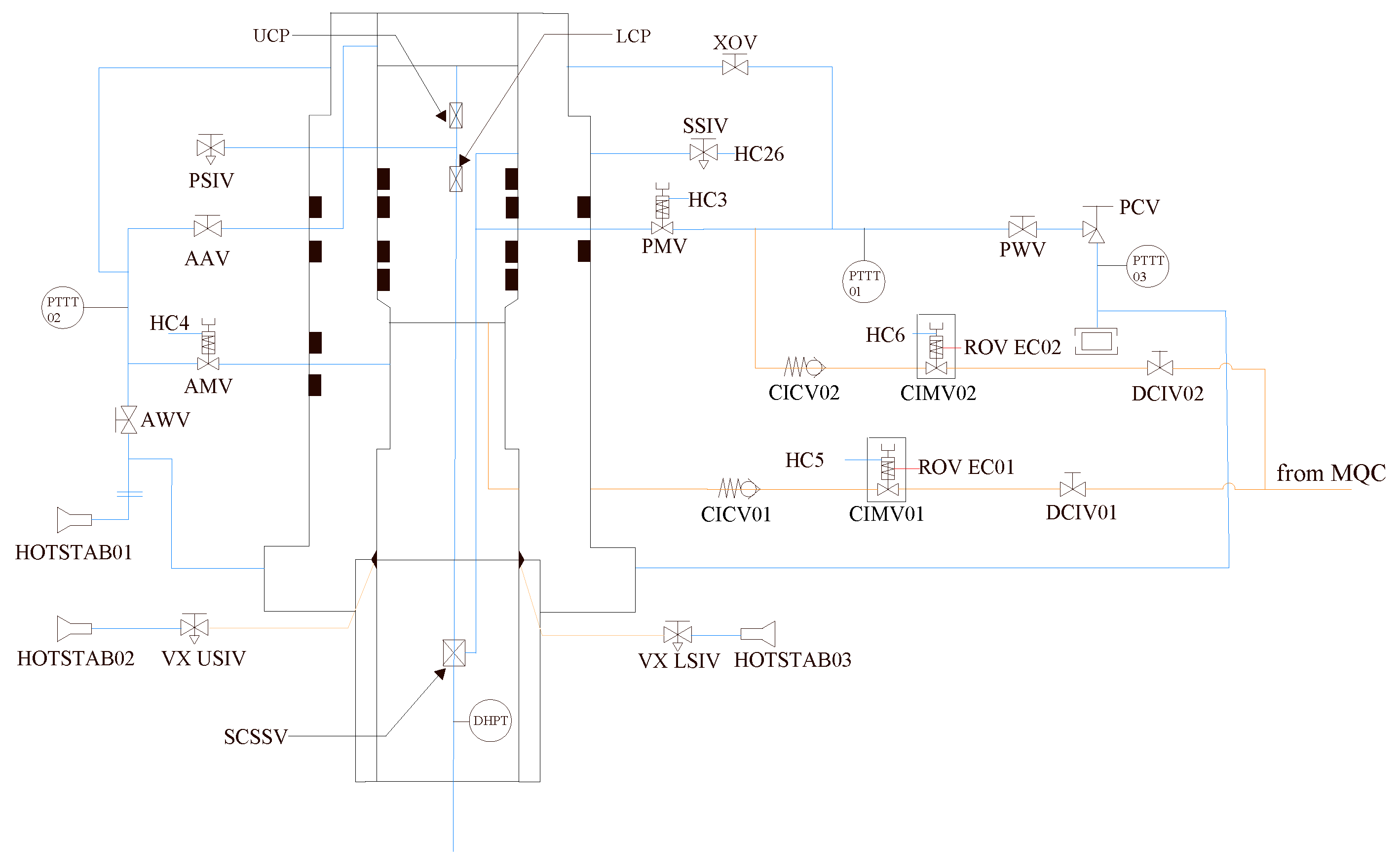
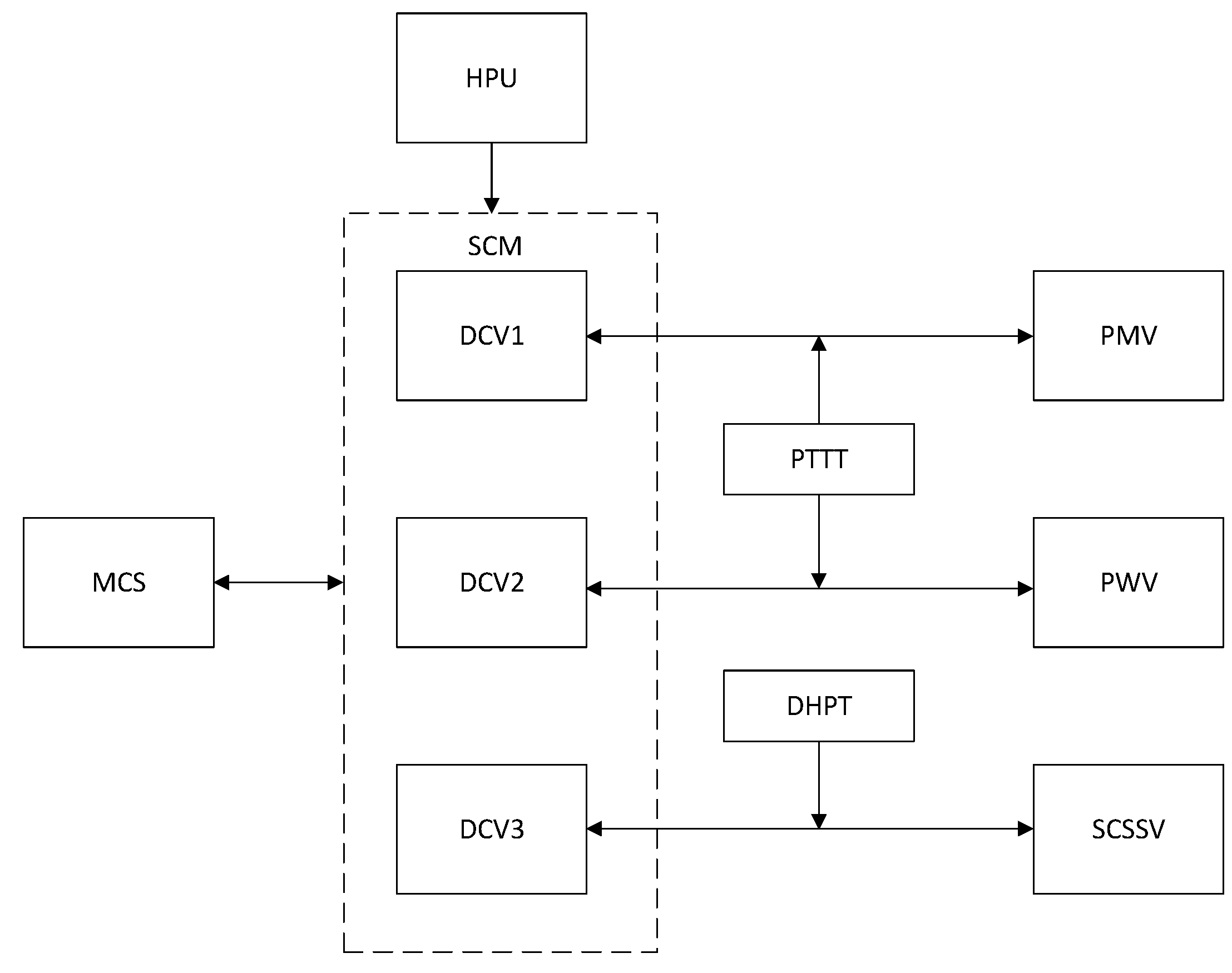
4.1. Reliability Model of Subsea Emergency Shutdown System Based on Time-Varying Failure Rate

Figure 7 shows the composition and function of the subsea ESD system [37], which performs the functions of both basic process control system (BPCS) and safety instrumented system (SIS) during oil and gas production. During normal production, the master control station (MCS) gives control instructions, and the offshore equipment opens the surface-controlled subsurface safety valve (SCSSV) through the SCM. The production master valve (PMV) and the production wing valve (PWV) remain normally open, and the subsea oil and gas are transmitted through the main loop pipeline. In case of production emergency, the temperature or pressure measured by the pressure transmitter and temperature transmitter (PTTT) will exceed the maximum limit. At this time, the hydraulic directional control valve controlled by SCM will lose power, forming oil return. The hydraulic oil pressure in the driver chamber of the PMV will decrease, then the reset spring closes the PMV. If the PPTT is still feeding back data, it will continue to close the PWV. In the event of pipeline leak or fire at production facility that cannot be prevented by the shutdown of the PMV and the PWV, the SCSSV will be closed to avoid a blowout and other accidents. When the SCSSV cannot be closed, the hydraulic power unit (HPU) will act directly to return the hydraulic oil to close the SCSSV.

When only considering the SIS function of the subsea ESD system shown in Figure 7, the reliability block diagram model of the system is established:

The subsea ESD system in Figure 8 is a hybrid system containing both series and parallel structures. The reliability model of this system is obtained by using the reliability calculation method of the series-parallel structure.

$$\begin{array}{c}{R}_{sys}=\left[(R_1+R_2-R_1{R}_2)R_3+R_4-(R_1+R_2-R_1{R}_2)R_3{R}_4\right]·R_5·\left[R_6{R}_7+R_8{R}_9\right.\hfill \\ \left.-R_6{R}_7{R}_8{R}_9+R_{10}{R}_{11}-(R_6{R}_7+R_8{R}_9-R_6{R}_7{R}_8{R}_9)R_{10}{R}_{11})\right]\hfill \end{array},$$

(34)

where $R_{sys}$ represents the reliability of the subsea ESD system, and $R_i$ represents the reliability of the equipment PTTT, DHPT, MCS, HPU, SCM, DCV1, PMV, DCV2, PWV, DCV3, and SCSSV of the system in turn.

• Equipment reliability model based on time-varying failure rate model before modification. The TFR model for each equipment of the subsea ESD system before modification is obtained using (4), then the reliability model of the equipment is as follows:

  $$R_i\left(t\right)=\left\{\begin{array}{cc}{e}^{-{\lambda }_{0,i}\mathrm{t}}\hfill & t\le T\\ exp\left(\frac{{\lambda }_{0,i}-{\lambda }_{0,i}{e}^{{\eta }_{0,i}(t-T)}}{{\eta }_{0,i}}\right)+e^{-{\lambda }_{0,i}T}-1\hfill & t>T\end{array}\right.,$$

  (35)
  When $i=1,2,\cdots ,11$, $R_i$, ${\lambda }_{0,i}$ and ${\eta }_{0,i}$, respectively, represent the reliability, failure rate in the steady state phase and the single value of failure rate cumulated parameter of the equipment PTTT, DHPT, MCS, HPU, SCM, DCV1, PMV, DCV2, PWV, DCV3, and SCSSV in this system.
• Equipment reliability model based on time-varying failure rate model after modification. The modified TFR model (14)–(17), for a given ${\alpha }_{0,i}$, when ${\eta }_i<{\eta }_{0,i}$,

  $$R_{\mathrm{i},mo}\left(t\right)=\left\{\begin{array}{cc}{e}^{-{\lambda }_{0,i}\mathrm{t}}\hfill & t\le T\\ exp\left(exp\left(\frac{{({\eta }_i-{\eta }_{0,i})}^{2}ln(1-{\alpha }_{0,i})}{{({\eta }_{L,i}^{{\alpha }_{0,i}}-{\eta }_{0,i})}^2}\right)·\frac{{\lambda }_{0,i}-{\lambda }_{0,i}{e}^{{\eta }_i(t-T)}}{{\eta }_i}\right)+e^{-{\lambda }_{0,i}T}-1\hfill & t>T\end{array}\right.$$

  (36)

  When ${\eta }_i>{\eta }_{0,i}$,

  $$R_{\mathrm{i},mo}\left(t\right)=\left\{\begin{array}{cc}{e}^{-{\lambda }_{0,i}\mathrm{t}}\hfill & t\le T\\ exp\left(exp\left(\frac{{({\eta }_i-{\eta }_{0,i})}^{2}ln(1-{\alpha }_{0,i})}{{({\eta }_{U,i}^{{\alpha }_{0,i}}-{\eta }_{0,i})}^2}\right)·\frac{{\lambda }_{0,i}-{\lambda }_{0,i}{e}^{{\eta }_i(t-T)}}{{\eta }_i}\right)+e^{-{\lambda }_{0,i}T}-1\hfill & t>T\end{array}\right.$$

  (37)

  Substituting the reliability model before and after modification of the equipment (35)–(37) into (34), the reliability models of the system based on the TFR model before and after modification are obtained.

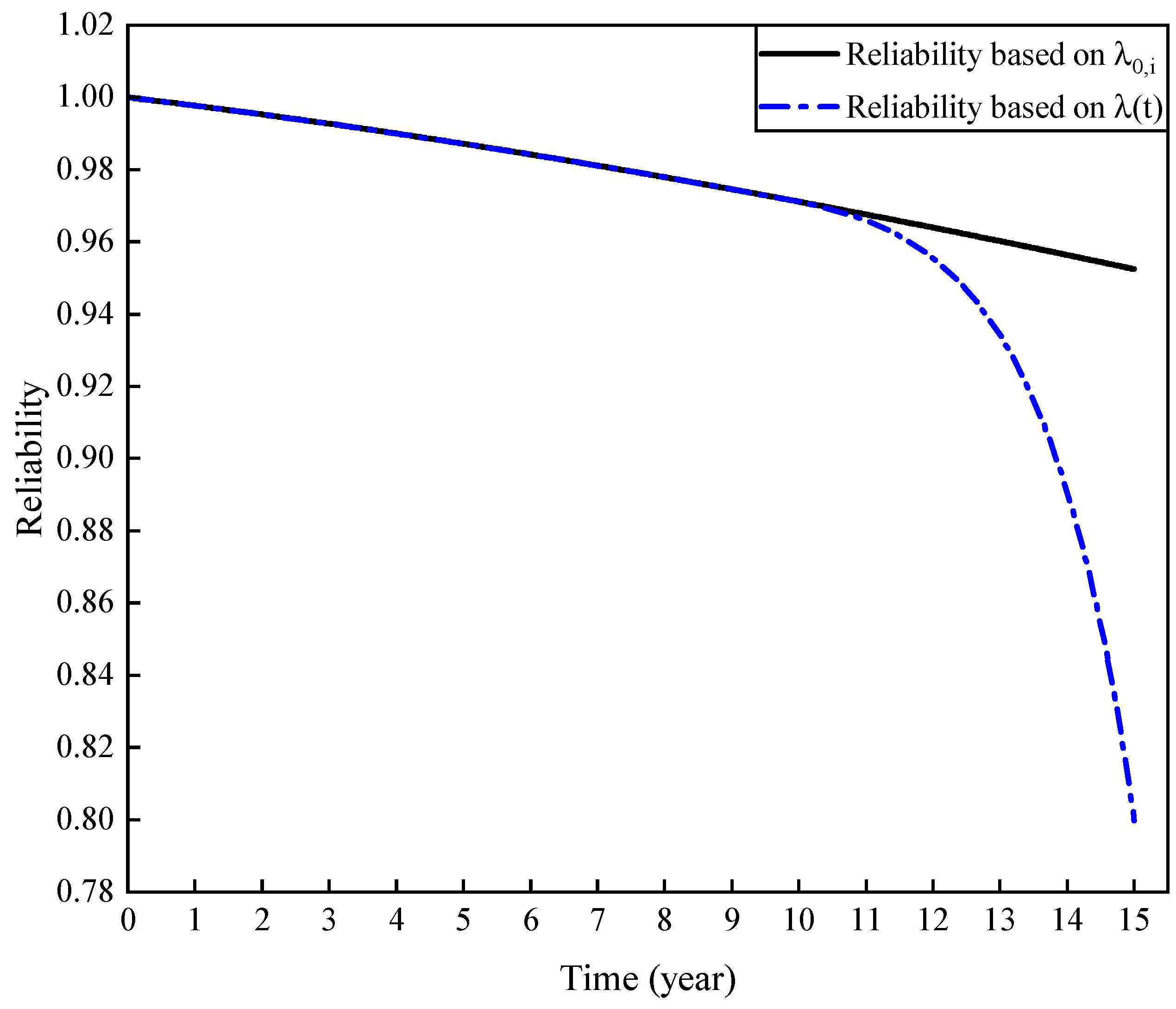
4.2. Reliability Comparison and Analysis Based on Time-Varying Failure Rate and Constant Failure Rate Models

As shown in

Table 2. Failure rate and failure rate cumulated parameter of each equipment in subsea emergency shutdown system.

Abbreviation	${\mathit{\lambda }}_{0,\mathit{i}}\left(\mathit{h}\right)$	${\mathit{\eta }}_{0,\mathit{i}}$	$\left[{\mathit{\eta }}_{\mathit{L},\mathit{i}}^{{\mathit{\alpha }}_{0,\mathit{i}}},{\mathit{\eta }}_{\mathit{U},\mathit{i}}^{{\mathit{\alpha }}_{0,\mathit{i}}}\right]$
PTTT	$3.88\times {10}^{-8}$	$0.000097$	$\left[0.000026,0.00012\right]$
DHPT	$1.85\times {10}^{-8}$	$0.000084$	$\left[0.000021,0.00011\right]$
MCS	$1.239\times {10}^{-10}$	$0.000055$	$\left[0.0000083,0.000078\right]$
HPU	$8.345\times {10}^{-9}$	$0.00007$	$\left[0.000012,0.000089\right]$
SCM	$2.511\times {10}^{-9}$	$0.00008$	$\left[0.000017,0.000099\right]$
DCV1	$5.3\times {10}^{-7}$	$0.0001$	$\left[0.000036,0.00014\right]$
PMV	$5.66\times {10}^{-8}$	$0.00015$	$\left[0.000053,0.00017\right]$
DCV2	$5.3\times {10}^{-7}$	$0.0001$	$\left[0.000036,0.00014\right]$
PWV	$5.66\times {10}^{-8}$	$0.00015$	$\left[0.000053,0.00017\right]$
DCV3	$5.3\times {10}^{-7}$	$0.0001$	$\left[0.000036,0.00014\right]$
SCSSV	$6.8\times {10}^{-7}$	$0.00018$	$\left[0.000064,0.00019\right]$

, the failure rate of each equipment ${\lambda }_{0,i}\left(h\right)$ in the subsea ESD system in the steady state phase refers to the OREDA, and the failure rate cumulated parameter is the expert experience value. The simulation is carried out in MATLAB, and the simulation time is 15 years, which is 131,400 hours. When considering the time-varying characteristics of failure rate, the first ten years is the steady state phase, and the failure rate increases with the passage of time in the last five years. Therefore, the T value in Equation (35) is 87,600 h.

The dot-dash line and the straight line in Figure 9 respectively represent the reliability curves of the subsea ESD system under TFR and CFR. When the time-varying characteristics of failure rate is considered, the system is in the steady state phase in the first ten years, and enters the wear-out phase in the tenth year. The aging of the components leads to an increase in the failure rate, and the system reliability decreases at a faster rate. The system reliability drops to 0.7995 in the fifteenth year when the failure rate cumulated parameter of each equipment is ${\eta }_{0,i}$. When the failure rate is constant, the system reliability drops to 0.9712 in the tenth year and 0.9524 in the fifteenth year. The comparison of reliability curves shows that the reliability of the system decreases too slowly when using the CFR and relatively faster when using the TFR. The reliability of the subsea ESD system drops to about 0.8 by the fifteenth year in engineering experience. The simulation result shows that the reliability evaluation of the system based on the TFR model is basically consistent with the engineering experience. It is too idealized to simplify the failure rate into a constant, which brings reliability evaluation error compared with TFR, and this error will get bigger and bigger over time. The TFR model in this paper eliminates this error.

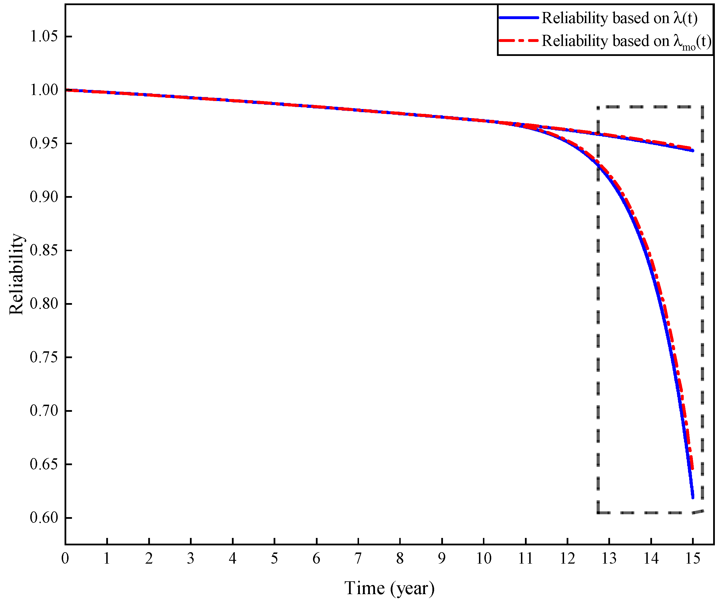
4.3. Reliability Comparison and Analysis of Time-Varying Failure Rate Models before and after Modification

The interval value $\left[{\eta }_{L,i}^{{\alpha }_{0,i}},{\eta }_{U,i}^{{\alpha }_{0,i}}\right]$ of the failure rate cumulated parameter is given in Table 2, where ${\alpha }_{0,i}$ is taken as a small range of 5%, which is estimated by the chi-square distribution for ${\eta }_{0,i}$. The upper and lower bounds of this interval are substituted into the TFR models before the modification during simulation, and the region of the system reliability curve which changes with the value of $\eta$ is obtained using Equation (35). In the simulation of the modified TFR model, the value of $\eta$ corresponding to the upper boundary is quickly obtained through the upper boundary existence theorem determined by the failure rate region. Based on Table 2 and the upper boundary existence theorem, the upper boundary of the modified failure rate region corresponds to the parameter ${\eta }_{U,i}^{{\alpha }_{0,i}}$.

The straight line and the dot-dash line in Figure 10, respectively, represent the reliability curves of the subsea ESD system based on the TFR models before and after modification. In the first ten years, the system is in the steady state phase, and enters the wear-out phase in the tenth year. The difference from the simulation in Section 4.2 is that the uncertainty of parameter $\eta$ is considered, and the reliability analysis result changes from a single value to an interval containing uncertainty, which is intuitively reflected in the expansion of the reliability curve from a single line to a region. The reliability interval of the system in the fifteenth year is $\left[0.9433,0.6188\right]$ based on the TFR model before modification. Based on the modified TFR model, the reliability interval of the system becomes $\left[0.9451,0.6412\right]$ in the fifteenth year. The comparison shows that the reliability curve decreases more slowly and the interval end values increase after the modification, which is because the TFR model before the modification ignores the confidence of $\eta$. The modified model solves this problem and makes the reliability interval containing uncertainty more accurate. The change trend of the curves in Figure 10 is consistent with that in Figure 5, which further reflects the precision of the model modification method and the upper boundary existence theorem. In fact, the lower bound of the system reliability interval cannot be infinitesimal or too small. It should be ensured that the reliability is meaningful in engineering applications. From the partial enlarged view, the lower bound of the reliability interval after modification in the partial enlargement diagram has a larger change range than the upper bound, and the lower bound is higher overall, indicating that the modification method fits the actual situation.

5. Conclusions

The failure rate of most equipment varies with time in long-term operation. In order to solve the problem of reliability evaluation error caused by constant failure rate, a new time-varying failure rate model is established after comprehensively considering the time-varying characteristics of the failure rate in the steady state phase and wear-out phase. The time-varying scale factor in the model included the failure rate cumulated parameters that influenced the curve trend. Due to the uncertainty of the failure rate cumulated parameter, a statistical-fuzzy model is established based on the interval of the failure rate cumulated parameter estimated by the parameter estimation combined with statistics and fuzzy knowledge. In addition, the TFR model is modified by using statistical-fuzzy model, which covers the confidence of the failure rate cumulated parameter, and changes the upper and lower boundaries of the region enclosed by the failure rate curves. To further explore the range of boundary variation, the upper boundary existence theorem for the failure rate region is proposed and demonstrated, so as to obtain the failure rate cumulated parameter when the failure rate changes fastest, and the theorem is applied to numerical example.

In this paper, the subsea emergency shutdown system which has been in marine environment for a long time is selected as the research object, and the reliability model is established by using time-varying failure rate model and system reliability block diagram. When the failure rate cumulated parameter is a single value, the reliability of the systems under time-varying failure rate and constant failure rate are compared and analyzed. When the failure rate cumulated parameter is an interval, combined with the upper boundary existence theorem for the failure rate region, the system reliability based on the time-varying failure rate models before and after the modification are compared and analyzed. The following conclusions are drawn.

• Compared with the constant failure rate, the system reliability with the time-varying failure rate decreases faster and reaches 0.7995 in the fifteenth year. The reliability in the fifteenth year in engineering experience is about 0.8, so the time-varying failure rate model proposed in this paper is consistent with the actual situation and can eliminate the reliability evaluation error caused by the constant failure rate.
• Compared with the model before the modification, the modified time-varying failure rate model has the confidence of $\eta$ attached, which increases the end value of the system reliability interval containing uncertainty, and the reliability interval obtained after the modification is more accurate and realistic.

In practical engineering, the system requires equipment maintenance based on reliability evaluation, so the reliability interval obtained from the modified failure rate model proposed in this study can theoretically provide data support for maintenance strategy and make it more flexible, and this work will be completed in the future.

References

1. Zhang, Y.; Tang, W.; Du, J. Development of subsea production system and its control system. In Proceedings of the 2017 4th International Conference on Information, Cybernetics and Computational Social Systems (ICCSS), Dalian, China, 24–26 July 2017; pp. 117–122. [Google Scholar] [CrossRef]
2. Lyalla, I.; Arulliah, E.; Innes, D. A critical analysis of open protocol for subsea production controls system communication. In Proceedings of the OCEANS 2017, Aberdeen, UK, 19–22 June 2017; pp. 1–7. [Google Scholar] [CrossRef] [Green Version]
3. Bai, Y.; Bai, Q. (Eds.) 7—Subsea Control. In Subsea Engineering Handbook, 2nd ed.; Gulf Professional Publishing: Boston, MA, USA, 2019; pp. 173–202. [Google Scholar] [CrossRef]
4. Hua, Y.; Kecheng, S.; Xin, D.; Chao, Y.; Yuanlong, Y. Adaptability Analysis of SubseaOil and Gas Control System in Bohai Sea Region. Mech. Electr. Eng. Technol. 2021, 50, 60–63, 137. [Google Scholar]
5. Yangfeng, F.; Guochu, C. Application of subsea electro-hydraulic control system in deepwater gas field project. China Pet. Chem. Stand. Qual. 2020, 40, 125–126. [Google Scholar]
6. Lu, W.; Weizhenq, A. Comparison and Analysis of Subsea Production Control System. Petrochem. Ind. Technol. 2018, 25, 17–19. [Google Scholar]
7. Nolan, D.P. (Ed.) Chapter 11—Emergency Shutdown. In Handbook of Fire and Explosion Protection Engineering Principles for Oil, Gas, Chemical, and Related Facilities, 4th ed.; Gulf Professional Publishing: Waltham, MA, USA, 2019; pp. 215–225. [Google Scholar] [CrossRef]
8. Wang, X.; Jia, P.; Lizhang, H.; Wang, L.; Yun, F.; Wang, H. Reliability and Safety Modelling of the Electrical Control System of the Subsea Control Module Based on Markov and Multiple Beta Factor Model. IEEE Access 2019, 7, 6194–6208. [Google Scholar] [CrossRef]
9. Pang, N.; Jia, P.; Wang, L.; Yun, F.; Wang, G.; Wang, X.; Shi, L. Dynamic Bayesian network-based reliability and safety assessment of the subsea Christmas tree. Process. Saf. Environ. Prot. 2021, 145, 435–446. [Google Scholar] [CrossRef]
10. Bae, J.H.; Shin, S.C.; Park, B.C.; Kim, S.Y. Design Optimization of ESD (Emergency ShutDown) System for Offshore Process Based on Reliability Analysis. MATEC Web Conf. 2016, 52, 10. [Google Scholar] [CrossRef] [Green Version]
11. Signorini, G.; Rigoni, E.; Rodrigues, M. Reliability Analysis Methodology for Oil and Gas Assets: Case Study of Subsea Control Module Operating in Deep Water Basin at Brazilian Pre-Salt. In Proceedings of the 2020 International Petroleum Technology Conference (IPTC), Dhahran, Saudi Arabia, 13–15 January 2020. [Google Scholar] [CrossRef]
12. Ismagilov, F.; Vavilov, V.; Karimov, R.; Yushkova, O.; Timofeev, A. Combined Method of Technical Analysis to Optimize the Aviation Electromechanical Systems Reliability Indicators. In Proceedings of the 2021 28th International Workshop on Electric Drives: Improving Reliability of Electric Drives (IWED), Moscow, Russia, 27–29 January 2021; pp. 1–4. [Google Scholar] [CrossRef]
13. Tang, Q.; Shu, X.; Zhu, G.; Wang, J.; Yang, H. Reliability Study of BEV Powertrain System and Its Components—A Case Study. Processes 2021, 9, 762. [Google Scholar] [CrossRef]
14. Tawfiq, A.A.E.; El-Raouf, M.O.A.; Mosaad, M.I.; Gawad, A.F.A.; Farahat, M.A.E. Optimal Reliability Study of Grid-Connected PV Systems Using Evolutionary Computing Techniques. IEEE Access 2021, 9, 42125–42139. [Google Scholar] [CrossRef]
15. Hassett, T.; Dietrich, D.; Szidarovszky, F. Time-varying failure rates in the availability and reliability analysis of repairable systems. IEEE Trans. Reliab. 1995, 44, 155–160. [Google Scholar] [CrossRef]
16. Retterath, B.; Venkata, S.; Chowdhury, A. Impact of time-varying failure rates on distribution reliability. In Proceedings of the 2004 International Conference on Probabilistic Methods Applied to Power Systems, Ames, IA, USA, 12–16 September 2004; pp. 953–958. [Google Scholar] [CrossRef]
17. Wang, R.; Xue, A.; Huang, S.; Cao, X.; Shao, Z.; Luo, Y. On the estimation of time-varying failure rate to the protection devices based on failure pattern. In Proceedings of the 2011 4th International Conference on Electric Utility Deregulation and Restructuring and Power Technologies (DRPT), Weihai, China, 6–9 July 2011; pp. 902–905. [Google Scholar] [CrossRef]
18. Abunima, H.; Teh, J. Reliability Modeling of PV Systems Based on Time-Varying Failure Rates. IEEE Access 2020, 8, 14367–14376. [Google Scholar] [CrossRef]
19. Zhang, Q.; Wang, X.; Du, W.; Zhang, H.; Li, X. Reliability Model of Submarine Cable Based on Time-varying Failure Rate. In Proceedings of the 2019 IEEE 8th International Conference on Advanced Power System Automation and Protection (APAP), Xi’an, China, 21–24 October 2019; pp. 711–715. [Google Scholar] [CrossRef]
20. Li, Q.; Wang, Z.; Zhao, H.; Liu, H.; Tian, L.; Zhang, X.; Qiu, J.; Xue, C.; Zhang, X. Research on Prediction Model of Insulation Failure Rate of Power Transformer Considering Real-time Aging State. In Proceedings of the 2019 IEEE 3rd Conference on Energy Internet and Energy System Integration (EI2), Changsha, China, 8–10 November 2019; pp. 800–805. [Google Scholar] [CrossRef]
21. Jian, L.; Feng, G.; Ming, Z.; Liuning, C.; Weiyao, L. Research on Optimal Inspection Strategy for Overhead Transmission Line Based on Smart Grid. Procedia Comput. Sci. 2018, 130, 1134–1139. [Google Scholar] [CrossRef]
22. Liu, H.; Wang, Z.; Han, M. Reliability Analysis of Solenoid Valve Power Supply Based on Time-Varying Fault Rate. In Proceedings of the 2019 4th International Conference on Mechanical, Control and Computer Engineering (ICMCCE), Hohhot, China, 25–27 October 2019; pp. 154–1543. [Google Scholar] [CrossRef]
23. Zhang, F.; Wu, M.; Hou, X.; Han, C.; Wang, X.; Liu, Z. The analysis of parameter uncertainty on performance and reliability of photovoltaic cells. J. Power Sources 2021, 507, 230265. [Google Scholar] [CrossRef]
24. Fan, L.; Lübin, P.; Tao, N.; Bo, H.; Kan, C.; Kunpeng, Z. A method for obtaining unknown reliability parameters of components based on simulated annealing algorithm. Electr. Meas. Instrum. 2021, 58, 1–10. [Google Scholar]
25. Wang, J.; Xu, Y.; Peng, Y.; Ye, Y. Estimation of Reliability Parameters of Protective Relays Based on Grey-three-parameter Weibull Distribution Model. Power Syst. Technol. 2019, 43, 1354–1360. [Google Scholar] [CrossRef]
26. Laure Miranda, F.; Willer de Oliveira, L.; Henriques Dias, B.; Chaves de Resende, L.; Geraldo Nepomuceno, E.; José de Oliveira, E. Composite Power System Reliability Evaluation Considering Stochastic Parameters Uncertainties. IEEE Lat. Am. Trans. 2020, 18, 2003–2010. [Google Scholar] [CrossRef]
27. Li, Z.; Yang, L.; Wang, D.; Zheng, W. Parameter Estimation of Software Reliability Model and Prediction Based on Hybrid Wolf Pack Algorithm and Particle Swarm Optimization. IEEE Access 2020, 8, 29354–29369. [Google Scholar] [CrossRef]
28. Wang, Z.; Pan, R. Point and Interval Estimators of Reliability Indices for Repairable Systems Using the Weibull Generalized Renewal Process. IEEE Access 2021, 9, 6981–6989. [Google Scholar] [CrossRef]
29. Uprety, I.; Patrai, K. Fuzzy Reliability Estimation Using Chi-Squared Distribution. In Proceedings of the 2016 3rd International Conference on Soft Computing Machine Intelligence (ISCMI), Dubai, United Arab Emirates, 23–25 November 2016; pp. 169–173. [Google Scholar] [CrossRef]
30. Yang, X.; Yang, Y.; Liu, Y.; Deng, Z. A Reliability Assessment Approach for Electric Power Systems Considering Wind Power Uncertainty. IEEE Access 2020, 8, 12467–12478. [Google Scholar] [CrossRef]
31. Wang, Z.; Shafieezadeh, A. On confidence intervals for failure probability estimates in Kriging-based reliability analysis. Reliab. Eng. Syst. Saf. 2020, 196, 106758. [Google Scholar] [CrossRef]
32. Hu, L.; Yue, D.; Zhao, G. Reliability Assessment of Random Uncertain Multi-State Systems. IEEE Access 2019, 7, 22781–22789. [Google Scholar] [CrossRef]
33. Li, X.Y.; Chen, W.B.; Li, F.R.; Kang, R. Reliability evaluation with limited and censored time-to-failure data based on uncertainty distributions. Appl. Math. Model. 2021, 94, 403–420. [Google Scholar] [CrossRef]
34. Wang, Y.; Li, W.; Zhang, P.; Wang, B.; Lu, J. Reliability Analysis of Phasor Measurement Unit Considering Data Uncertainty. IEEE Trans. Power Syst. 2012, 27, 1503–1510. [Google Scholar] [CrossRef]
35. Rausand, M. (Ed.) Chapter 2—Failure Model. In System Reliability Theory: Models, Statistical Methods, and Applications, 2nd ed.; National Defense Industry Press: Beijing, China, 2010; pp. 6–37. [Google Scholar]
36. Xianhui, Y.; Haitao, W. Chapter 5—Reliability Model and Failure Data. In Functional Safety of Safety Instrumented Systems; Tsinghua University Press: Beijing, China, 2007; pp. 78–95. [Google Scholar]
37. Bodsberg, L. Application of IEC 61508 and IEC 61511 in the Norwegian Petroleum Industry; The Norwegianoil Industry Association: Oslo, Norway, 2004; pp. 81–109. [Google Scholar]
Figure 1. Diagram of bathtub curve.
Processes 09 02214 g001
Figure 2. Diagram of the PG membership function for failure rate cumulated parameter.
Processes 09 02214 g002
Figure 3. Time-varying failure rate curves under different failure rate cumulated parameter.
Processes 09 02214 g003
Figure 4. Reliability block diagram of the pressure vessel safety instrument system.
Processes 09 02214 g004
Figure 5. Comparison of reliability curves of the pressure vessel safety instrument system models before and after modification.
Processes 09 02214 g005
Figure 6. Layout of valves and instruments of the control system located in the tree and downhole.
Processes 09 02214 g006
Figure 7. Function diagram of subsea emergency shutdown system.
Processes 09 02214 g007
Figure 8. Reliability block diagram of subsea emergency shutdown system.
Processes 09 02214 g008
Figure 9. Reliability curves comparison diagram based on time-varying failure rate and constant failure rate.
Processes 09 02214 g009
Figure 10. Reliability curves comparison diagram based on time-varying failure rate models before and after modification.
Processes 09 02214 g010