Dynamic Prediction of Chilo suppressalis Occurrence in Rice Based on Deep Learning

Abstract

(1) Background: The striped rice stem borer (SRSB), Chilo suppressalis, has severely diminished the yield and quality of rice in China. A timely and accurate prediction of the rice pest population can facilitate the designation of a pest control strategy. (2) Methods: In this study, we applied multiple linear regression (MLR), gradient boosting decision tree (GBDT), and deep auto-regressive (DeepAR) models in the dynamic prediction of the SRSB population occurrence during the crop season from 2000 to 2020 in Hunan province, China, by using weather factors and time series of related pests. (3) Results: This research demonstrated the potential of the deep learning method used in integrated pest management through the qualitative and quantitative evaluation of a reasonable validating dataset (the average coefficient of determination ${\mathrm{R}}_{\mathrm{mean}}^2$ for the DeepAR, GBDT, and MLR models were 0.952, 0.500, and 0.166, respectively). (4) Conclusions: The DeepAR model with integrated ground-based meteorological variables, time series of related pests, and time features achieved the most accurate dynamic forecasting of the population occurrence quantity of SRSB as compared with MLR and GBDT.

1. Introduction

The Chilo suppressalis (striped rice stem borer, hereafter referred to as SRSB), the most widely distributed and destructive rice pest [1], is also the worst rice pest in China [2]. The larvae of SRSB eat rice stems, which leads to rice with dead hearts in the tillering stage, then forms white earheads during the heading stage, which can finally lead to rice with dead sheath [3] (Figure 1). Annually, China suffers severe rice yield reduction and economic losses from the SRSB pest [3,4,5,6]. This destruction is caused in part by the rapid proliferation of pests within pest populations, which makes it difficult for farmers to predict its outbreak. Continuously monitoring and accurately predicting the dynamic changes in the pest population during the crop growth period may be helpful for protecting rice from SRSB.

The insect population can be affected by many factors; both abiotic and biotic factors are believed to be responsible for changes in the insect population [1]. The effects of abiotic factors such as climate variables have been well-documented [7]. Therefore, an adequate early warning of an SRSB infestation combined with meteorological factors can support plant protection efforts. Apart from being threatened by SRSB, rice is also negatively affected by various pests such as the rice planthopper (hereafter referred to as RPH) and the paddy leaf roller (hereafter referred to as PLR). Thus, the species and the numbers of other pests in the region will also have effects on the population development trends for SRSB.

An agricultural pest prediction model is built on the pest occurrence mechanism, mathematical statistics, time series analyses, together with the critical factors affecting pest occurrence, which can provide information on pest occurrence, severity, and development trends. Differentiated by the principles of prediction methods, the current range of pest prediction models include statistical regression models, machine learning models, and deep learning models.

Statistical modeling for the early prediction of pest risks is one strategy that has been widely adopted [8], and whose essence is to ascertain the relationships between variables in the form of fitting equations. The predicting steps involve: performing a statistical analysis with the historical data on pests, extracting the relationship between the target pests $y$ and a related factor $x$, establishing the mathematical equations, and then making a quantitative prediction of pests by means of these equations. This kind of prediction approach treats pest occurrence as a separate system, without considering the occurrence process and mechanism. The most commonly used approach is the multiple linear regression (MLR) model. The severe difficulty for statistical regression methods lies in choosing the relevant factor $x$; most researchers currently tend to build predicting models with relevant meteorological factors [9,10]. Some researchers have found that combining weather factors with other factors, such as variety, soil, fertilization, etc., can improve a model’s prediction capability [11,12]. The statistical learning-based methods focusing on finding the linear relations between variables have high interpretability. However, most problems in real-life production show rich, non-linear links for which traditional statistical regression methods do not work.

The machine learning method has a strong predictive capability that automates the organization, fits the parameter adjustment model, obtains the optimal model to fit the current datasets, and predicts with the optimal model. The accuracy and speed of the machine learning method improve as the amount of data increases, which is what distinguishes it from traditional statistical regression methods. The machine learning method can also learn non-linear relationships; consequently, the machine learning-based regression analysis has become the mainstream in agricultural pest prediction, with support vector machines [13] and decision trees [10] as the two commonly adopted machine learning prediction algorithms. However, machine learning algorithms are so diverse that it is difficult for researchers to choose one for practical problems. Moreover, the pros and cons of machine learning algorithms also differ, such as the SVM being inefficient in processing large samples of data [14], while the performance of neural networks improves with an increase in data volume [15], but which also easily leads to higher computational costs and the overfitting of traditional neural networks [16].

Deep learning, a branch of machine learning, is an algorithm using the artificial neural networks as an architecture to characterize and learn data [17,18,19,20,21]. The algorithm is extensively applied in most traditional fields [22,23,24,25], and some progress has been made in the field of agricultural pest prediction in recent years [26]. With the reduction of hardware costs and the improvement of algorithms, deep learning-based methods will become a leading research topic for agricultural pest prediction.

Aiming at the prediction of SRSB occurrence in rice, and combining this with ground meteorological observation data and related pest time sequence data, this paper constructs a multi-dimensional dynamic probability prediction model based on the use of deep learning for time series analyses. The model presented in the paper is more applicable than the traditional pest prediction models and can realize a dynamic timing prediction of pests. The key works included in the paper are as follows: (1) investigating the relationships between ground meteorological data, related pests, and SRSB; (2) comparing the performances of the models using only meteorological variables to that of the models combining meteorological variables with the time series of related pests; (3) developing a deep learning-based dynamic probability prediction DeepAR model for the occurrence of SRSB; (4) evaluating the performance of the DeepAR model using the traditional MLR model and the machine learning GBDT model.

Our method is expected to lead to an improved method for the management of SRSB for following reasons:

(1)

Our study suggests that combining related pest time series data with the ground meteorological data can improve the model’s prediction accuracy as compared to previous studies using only the ground meteorological data;

(2)

Combining weather and associated pest time series with deep learning-based DeepAR models can provide more accurate predictions than the traditional MLR and the machine learning GBDT. These findings could be utilized to support an integrated pest management (IPM) program to help farmers reduce the use of pesticides and minimize crop loss in rice paddy fields.

2. Materials and Methods

2.1. Study Areas

This paper mainly studied the dynamic population change of SRSB in Hunan Province, China, and the area selection was based on the following considerations:

• Areas have a high number of insects;
• Areas have a long history of rice cultivation;
• Area characteristics can represent different regions in Hunan Province, China.

Based on these, A (Hongjiang), B (Yuangjiang), C (Dong’an), D (Linli), and E (Liling) were selected as the study areas (Figure 2). Hunan Province belongs to an area with the most extensive rice farming in China. The selected area has high temperatures and is rainy in summer and hot at the same time, which is suitable for the occurrence of SRSB.

2.2. Data Collection

2.2.1. Pest Data

The pest data came from the daily records of the rice pest light traps for major insect pests in the crop monitoring and early warning information system in Hunan Province, China. Pest species include 11 rice pests (

Table 1. The main rice pests captured by the light traps.

Number	Name	Abbreviation	Latin Name
0	rice planthopper	RPH	-
1	paddy leaf roller	PLR	Cnaphalocrocis medinalis
2	striped rice stem borer	SRSB	Chilo suppressalis
3	pink sugarcane borer	PSB	Sesamia grisescens
4	yellow stem borer	YSB	Scirpophaga incertulas
5	rice green semilooper	RGS	Naranga diffusa
6	rice plant weevil	RPW	Echinocnemus squameus
7	rice water weevil	RWW	Lissorhoptrus oryzophilus
8	gall midge	GM	Orseoia oryzae
9	paddy armyworm	PA	Mythimna separata
10	-	Other *	-

* ‘Other’ is the sum of other species captured by our light traps apart from the rice pests shown (Numbers 0–9).

), such as SRSB, RPH, and PLR. Adult pests were collected by a light trap set from 18:00 to 6:00 the next day, located in areas A (2000–2020), B (2000–2020), C (2000–2020), D (2000–2020), and E (2010–2020). Plant protection workers removed the insects from the traps every morning, and subsequently identified and counted them.

2.2.2. Meteorological Data

Meteorological data were obtained from the ground daily meteorological data downloaded by the National Meteorological Center, spanning the years 2000–2020, including 19 factors such as temperature, precipitation, and sunshine duration; the detailed information is shown in

Table 2. Types and units of meteorological factors.

Number	Type	Abbreviation	Unit	Number	Type	Abbreviation	Unit
0	Temperature	TEMP	°C	10	Precipitation	PRCP	mm
1	Maximum temperature	Tmax	°C	11	Evaporation	EVP	mm
2	Minimum temperature	Tmin	°C	12	Atmospheric pressure	AP	pa
3	Average relative humidity	RH	%	13	Maximum atmospheric pressure	APmax	pa
4	Minimum relative humidity	RHmin	%	14	Minimum atmospheric pressure	APmin	pa
5	Wind speed	WDSP	m/s	15	Skin temperature	SKT	°C
6	Maximum wind speed	MXWDSP	m/s	16	Maximum skin temperature	SKTmax	°C
7	Maximum wind direction	MXWDD	16 directions	17	Minimum skin temperature	SKTmin	°C
8	Extreme wind speed	EXWDSP	m/s	18	Sunshine duration	SDD	H
9	Extreme wind direction	EXWDD	16 directions

.

2.2.3. Time Features

As pest occurrence is a typical time series problem, it has prominent temporal characteristics. The extraction of the time characteristics of pest data facilitates the construction of more accurate predictive models. We extracted the time features, including years, seasons, months, weeks, weekdays, and days. Among these were March–May for spring, June–August for summer, September–November for autumn, and from December to the following February for winter. The weeks were composed of seven days as one week, with 52 weeks per year. Weekdays entailed the obtainment of working day information according to the Gregorian calendar, mainly considering that the acquisition of pest data required manual recording.

2.2.4. Data Preprocessing

The original pest data had some missing and outlier values. The missing values were interpolated using the average adjacent position interpolation method. We selected the five previous and five subsequent effective values of the missing fraction to calculate the arithmetic mean, and used this arithmetic mean to interpolate the missing part. The outliers were processed using the exponentially weighted averages method, and the exponentially weighted averages were defined as follows:

$$y_t=\frac{x_t+\left(1-\alpha \right)x_{t-1}+{\left(1-\alpha \right)}^2{x}_{t-2}+\cdots \cdots +{\left(1-\alpha \right)}^t{x}_0}{1+\left(1-\alpha \right)+{\left(1-\alpha \right)}^2+\cdots \cdots +{\left(1-\alpha \right)}^t},$$

(1)

where $\alpha$ is the smoothing factor $(\alpha \in \left(0,\left.1\right]\right)$, $y_t$ is the value after $t$ moment smoothing, $x_t$ is the value before $t$ moment smoothing. In this paper, a sliding window with seven days as a window and one day as a step were established to smooth the pest data.

The meteorological data were processed in the same way. There were no meteorological stations in some parts of the study area. This paper used meteorological stations near cities and counties in the study area (

Table 3. The study areas and the corresponding meteorological stations.

Number	Study Area	Meteorological Stations
0	Liling	Zhuzhou
1	Hongjiang	Zhijiang Dong Autonomous County
2	Dong’An	Lingling
3	Yuanjiang	Yuanjiang
4	Linli	Shimen

).

Some time series of related pests contain unique values. Unique values do not help with model construction. In addition, there is a collinearity relationship among some variables. Collinearity plays a consistent role in the process of model construction, where it raises the complexity of the model. Therefore, we removed the unique values and excess collinearity variables during the model construction. In this paper, high-quality pest variables, meteorological variables, and time datasets (

Table 4. Rice pests, weather, and time datasets.

Weather Variables		Time Series of Related Pests	Time Features
TEMP	EVP	RPH	Year
RH	AP	PLR	season
RHmin	PRCP	SRSB	month
WDSP	EXWDD	PSB	weeks
MXWDSP	EXWDSP	YSB	-
MXWDD	SDD	-	-
SKTmax	-	-	-

) were constructed, laying the material basis for the subsequent analysis and prediction.

2.3. Methods

2.3.1. Datasets Preparation

To predict the SRSB, weather variables (including TEMP, RH, and PRCP) and the associated time series of related pests were included as input variables. Furthermore, the daily SRSB light trap catches were natural log-transformed before analysis to satisfy the regression hypothesis [27,28]. The SRSB light trap catches were treated as an output variable in all models and an input variable in the autoregressive model.

The datasets of all variables of crop seasons in E (Liling) from 2010 to 2019, and those of other study areas from 2000 to 2018 were used as training datasets. E (Liling) training datasets contained 3726 samples, and other study areas’ training datasets contained 7013 samples. In Liling 2020, the remaining observations from other regions from 2019 to 2020 were used as test datasets to verify the model. We chose data from March to October to develop the models, as this period was commonly used to plan pest monitoring. All the details are summarized in

Table 5. Details of the data used in model development.

Site	Place	Input Variable	Output Variable	Month (Yearly)	Training Data	Testing Data
A	Hongjiang	Weather variables, Time series of related pests, and Time features	Chilo suppressalis (SRSB)	March to October	2000 to 2018	2019 to 2020
B	Yuanjiang				2000 to 2018	2019 to 2020
C	Dong’an				2000 to 2018	2019 to 2020
D	Linli				2000 to 2018	2019 to 2020
E	Liling				2010 to 2019	2020

.

2.3.2. Model

Multiple Linear Regression (MLR)

Pearson correlation analysis was used to obtain the relationship between SRSB and meteorological data, associated pest time series, and time features. Taking the significant correlation coefficient (R) as the standard, we selected appropriate variables to develop the linear model of SRSB.

An MLR model using stepwise selection was established in three scenarios: (1) only meteorological variables were considered to estimate the maximum determination coefficient of the SRSB (the R square); (2) meteorological variables and time series-related pests were combined to estimate the maximum determination coefficient of the SRSB (the R square); (3) meteorological variables, time series-related pests, and time features were considered to estimate the maximum determination coefficient of the SRSB (the R square).

MLR is a statistical method of regression for analyzing the relationship of an individual dependent variable with two or more independent variables [29], which can be demonstrated as follows:

$$y={\alpha }_0+{\alpha }_1{x}_1+{\alpha }_2{x}_2+\cdots +{\alpha }_i{x}_i\cdots +{\alpha }_k{x}_k+\epsilon ,$$

(2)

Here $y$ is the dependent variable, $x_i$ is the independent variable, ${\alpha }_0$ represents the intercept, ${\alpha }_i$ is the slope of $x_i$ to $y$, $\epsilon$ is the residual. Stepwise regression can automatically select the most relevant independent variables when the number of independent variables is large and where it is noted possible to fit all potential models [30]. We used Python’s statsmodels library to implement the MLR model.

Gradient Boosting Decision Tree (GBDT)

The GBDT or the Gradient Boosting Decision Tree, an ensemble model of an iterative decision tree algorithm proposed by Jerome Friedman in 1999, is a representative model of the ensemble method. GBDT takes the regression tree as a base learner, integrated gradient boosting algorithm [31].

To train the GBDT model, we used a grid search combined with a 5-fold cross-validation [32]. The GBDT model was parameter-optimized to obtain the best performing GBDT model under the current datasets. The training and test datasets contained all variables (meteorological, related pest, and time features). We selected the model with the highest R² as the best GBDT model, calculating and plotting the importance of the input variables. This model was developed using the LightGBM library of python.

DeepAR Model

DeepAR is a probabilistic prediction method based on auto-regression recurrent neural networks. The approach solves the prediction problem through deep neural network learning by combining the appropriate likelihood, using non-linear data transformation techniques. DeepAR takes advantage of LSTM-based recurrent neural network architecture [33,34]. It also builds on previous deep learning work on time-series data [35,36,37] to address the probabilistic prediction problem. Deep networks, allowing for more abstract data representation through more complex transformations [21], thus generally outperform shallow and broad neural networks.

DeepAR has the following advantages: First, it performs a probabilistic prediction of the sample using the Monte Carlo method and can calculate consistent quantile estimates across all sub-ranges in the predicted range. Secondly, the method does not assume Gaussian noise, but broad likelihood functions can be supported and allow users to select the parts most suitable for the statistical data properties. Once again, by learning from similar data, being able to provide predictions from data with little or no history is something that conventional one-dimensional predictions cannot do. Finally, DeepAR can understand seasonal behavior and complex dependencies with minimal human intervention [38].

Through the use of the deep learning DeepAR time series prediction model, combining the time series of related pests, meteorological variables, and time features to predict the daily capture of SRSB light traps produced training and test datasets that contained all variables (meteorological, pest, and time).

We used the Gluonts library based on the MXNet framework to build the DeepAR model of the rice SRSB, selected the negative binomial distribution as the likelihood function of the DeepAR model; all the other hyperparameters used the default hyperparameters.

2.3.3. Evaluation Metrics

Multiple metrics can be used to analyze the performance of our prediction, so we opted to use the top 4 most used metrics for time series forecasting. We used the Coefficient of Determination (R²), Mean Absolute Error (MAE), Symmetric Mean Absolute Percentage Error (sMAPE), and Root Mean Square Error (RMSE) to evaluate the prediction model.

Coefficient of Determination (R²)

R² was used to measure the proportion of various independent variables that independent variables could explain to judge the explanatory power of the regression model [39,40,41].

Suppose that a dataset includes $y_1,\cdots \cdots , y_n$ total $n$ observations, the corresponding model of predicted values is thus $f_1,\cdots \cdots , f_n$. Defining the residual with $e_i=y_i-f_i$, the average observed value is calculated as follows:

$$y={\alpha }_0+{\alpha }_1{x}_1+{\alpha }_2{x}_2+\cdots +{\alpha }_i{x}_i\cdots +{\alpha }_k{x}_k+\epsilon ,\overline{y}=\frac{1}{n}{\sum }_{i=1}^n{y}_i,$$

(3)

The total sum of the square can thus be obtained with:

$$S{S}_{tot}={\sum }_i{\left(y_i-\overline{y}\right)}^2,$$

(4)

The sum of the squares of residuals can be calculated with the following formula:

$$S{S}_{res}={\sum }_i{\left(y_i-f_i\right)}^2={\sum }_i{e}_i^2,$$

(5)

Thus, the determination coefficient can be defined as follows:

$${\mathrm{R}}^2=1-\frac{S{S}_{res}}{S{S}_{tot}},$$

(6)

The ${\mathrm{R}}^2$ usually ranges from 0 to 1. The ${\mathrm{R}}^2$ can be more truthful than sMAPE, MAE, MAPE, MSE, and RMSE in regression analysis evaluation [42].

Mean Absolute Error (MAE)

MAE refers to the meaning of the distance between the predictive model value $f_i$ and the true value $y_i$ of the sample. MAE is calculated as:

$$MAE=\frac{1}{n}{\sum }_{i=1}^n\left|y_i-f_i \right|,$$

(7)

Symmetric Mean Absolute Percentage Error (sMAPE)

sMAPE is an accuracy measure based on percentage (or relative) errors. It is usually defined as follows:

$$sMAPE=\frac{100\%}{n}{\sum }_{i=1}^n\frac{\left|f_i-y_i\right|}{(|f_i|+\left|y_i\right|)/2},$$

(8)

Root Mean Square Error (RMSE)

RMSE is widely used to measure the differences between values predicted by a model and the values observed. It is defined as follows:

$$sMRMSE=\sqrt{\frac{1}{n}{\sum }_{i=1}^n{\left(f_i-y_i\right)}^2},$$

(9)

In general, lower MAE, sMAPE, and RMSE are better than higher values, and all three metrics are non-negative. But for the R², higher is better.

3. Results

3.1. Relationship between Climatic Variables, Time Series of Related Pests, and Time Features, and the SRSB Light Trap Catch

The correlation coefficient (R) was calculated between the natural log-transformed SRSB light trap catch and the selected environmental variables (climatic variables, related pest, and time features), and the correlation coefficient (R) and sig. (p > |t|) were calculated for five study regions and then averaged (

Table 6. Pearson’s correlation coefficient (R) between the natural log-transformed SRSB light trap catch and its associated pest, meteorological, and time features from March to October in the rice crop season.

Variable Types	External Variables	Correlation Coefficient (R)	Sig. (p > |t|)
Related pests	RPH	0.458 ± 0.111	0.008 ± 0.011 *
	PLR	0.368 ± 0.068	0.123 ± 0.179
	PSB	0.271 ± 0.098	0.000 ± 0.000 **
	YSB	0.086 ± 0.029	0.119 ± 0.265
Weather	TEMP	0.449 ± 0.046	0.213 ± 0.374
	RH	−0.031 ± 0.047	0.048 ± 0.235
	RHmin	−0.041 ± 0.064	0.082 ± 0.133
	WDSP	0.049 ± 0.136	0.052 ± 0.048
	MXWDSP	0.161 ± 0.083	0.121 ± 0.131
	MXWDD	0.086 ± 0.161	0.335 ± 0.364
	EXWDSP	0.175 ± 0.061	0.352 ± 0.355
	EXWDD	0.098 ± 0.155	0.334 ± 0.291
	SDD	0.282 ± 0.013	0.112 ± 0.174
	PRCP	0.091 ± 0.039	0.090 ± 0.121
	EVP	0.409 ± 0.033	0.073 ± 0.163
	AP	−0.445 ± 0.070	0.013 ± 0.029 *
	SKT	0.469 ± 0.050	0.208 ±0.209
Time	Weeks	0.112 ± 0.042	0.562 ± 0.264
	Month	0.113 ± 0.041	0.477 ± 0.238
	Year	0.146 ± 0.087	0.191 ± 0.418
	Season	−0.247 ± 0.079	0.001 ± 0.001 *

** Extremely significant, * significant.

). Our results show that the SRSB light trap catch had a significant positive correlation with the RPH light trap catch (R = 0.458 ± 0.111, p > |t|), and had an extremely significant positive correlation with the PSB light trap catch (R = 0.271 ± 0.098, p > |t|), but had a significant negative correlation with AP (R= −0.445 ± 0.070, p > |t|) and the season (R = −0.247 ± 0.079, p > |t|). Meanwhile, it there was some correlation between the SRSB light trap catch and the TEMP, SDD, and PLR light trap catch, but not significant. Extremely significant and significant correlation variables were included in the linear and non-linear models to predict SRSB light trap catches.

3.2. Multiple Linear Regression Prediction

Using a stepwise selected MLR model, we combined meteorological, associated pest, and time features (

Table 7. Statistical diagnostics of the stepwise multiple linear regression models (taking the Yuanjiang SRSB as an example).

Model	Variables	Coef	Std Err	t	$\mathit{p}>\left|\mathit{t}\right|$	VIF < 3
Weather	Const.	708.1329	11.604	61.026	0.000
	AP	−61.3799	1.007	−60.977	0.000	True
		N = 7013	R2 = 0.347	Adj.R2 = 0.346
Weather and related pests time series	Const.	536.1561	13.543	39.591	0.000
	AP	−46.4895	1.175	−39.568	0.000	True
	RPH	0.1205	0.006	19.113	0.000	True
	YSB	2.1725	0.194	11.182	0.000	True
	PSB	0.4584	0.043	10.694	0.000	True
		N = 7013	R2 = 0.3998	Adj.R2 = 0.399
Weather, time series of related pests, and time features	Const.	535.9426	13.535	39.589	0.000
	AP	−45.5927	1.210	−37.688	0.000	True
	RPH	0.1283	0.007	18.889	0.000	True
	YSB	2.1272	0.195	10.924	0.000	True
	PSB	0.4709	0.043	10.943	0.000	True
	Season	−0.0050	0.002	−3.067	0.002	True
		N = 7013	R2 = 0.400	Adj.R2 = 0.400

). $Coef$ is the MLR model coefficient that indicates the contribution of each variable to the model. $std err$ is the standard error of the coefficient estimation. $t$ and $p>\left|t\right|$ represent the effects of the independent variable on the dependent variable. The meteorological variable AP was significantly and negatively correlated with the SRSB light trap catch. Related pest RPH, YSB, and PSB with the light trap catch and the time variable season were negatively correlated with the SRSB light trap catch.

The use of meteorological variables (Model 1) alone explain approximately 35% (Adj.R² = 0.346) of the variability in the SRSB light trap catch; the model based on meteorological variables and related pest (Model 2) explains 39.9% (Adj.R² = 0.399) of the variability in the SRSB light trap capture; in comparison, a model based on meteorological variables, associated related pests, and time features (Model 3) could explain 40% (Adj.R² = 0.400) of the variability in the SRSB light trap catch. The variance inflation factor (VIF) for all the input variables was less than three, indicating no multiple collinearities among the variables. The adjusted R² selected the model combining meteorological variables, associated pests, and time features (Model 3) as the best model.

According to the results of the stepwise regression shown in Table 7, the prediction model of the Yuanjiang can be represented using the following regression equation:

$$\begin{array}{c}ln\left(SRSB\right)535.9426+\left(-45.5917\times AP\right)+\left(0.1283\times RPH\right)+\left(0.4709\times PSB\right)+\left(2.1272\times YSB\right)+\\ \left(-0.005\times Season\right),\end{array}$$

(10)

The dependent variable ln(SRSB) indicates the natural logarithm of the SRSB light trap catch. The independent variables AP, RPH, PSB, YSB, and Season indicate the AP, RPH light trap catch, PSB light trap catch, YSB light trap catch, and Season, respectively.

The MLR model of the other SRSB light trap catch of the study area was obtained using the same method, and a summary of the MLR model for the training datasets of each study area is shown in

Table 8. Summary of the MLR model for the training datasets of each study area.

	Place	Yuanjiang (R2 = 0.400, Adj.R2 = 0.400, N = 7013)	Hongjiang (R2 = 0.379, Adj.R2 = 0.378, N = 7013)	Dong’an (R2 = 0.398, Adj.R2 = 0.398, N = 7013)	Linli (R2 = 0.257, Adj.R2 = 0.256, N = 7013)	Liling (R2 = 0.359, Adj.R2 = 0.358, N = 3726)
Variable
Const.		535.943	2.146	0.425	−0.489	−0.952
TEMP		0	0	0.071	0.494	0.701
RHmin		0	−0.412	0	0	0
AP		−45.592	0	0	0	0
RPH		0.128	0.209	0.258	0	0
PSB		0.471	0.759	0	2.123	0.430
YSB		2.127	−0.235	3.359	0.169	3.070
PLR		0	0	0	0.054	0.397
Season		−0.005	−0.134	−0.165	−0.159	−0.175
Weeks		0	−0.007	0	0	0
Month		0	0	−0.030	0	0

. R² and Adj.R² represent the MLR fitting accuracy of the training datasets, and N represents the length of the training datasets. The results show that in different study regions, stepwise regression selected different independent variables.

The average coefficient of determination, minimum coefficient of determination, and maximum coefficient of determination of the MLR model based on the test dataset in the study areas (Linli, Liling, Yuanjiang, Dong’an, and Hongjiang) are ${\mathrm{R}}_{\mathrm{mean}}^2=0.166$, ${\mathrm{R}}_{\min }^2=0.083$, and ${\mathrm{R}}_{\max }^2=0.312$, respectively.

3.3. GBDT Model Prediction

Based on the training dataset, the GBDT models from different study regions (Linli, Liling, Yuanjiang, Dong’an, and Hongjiang) yielded other results (R² = 0.420, 0.104, 0.639, 0.509, and 0.564, RMSE = 0.999, 1.799, 0.860, 1.078, and 0.733). Figure 3 shows the GBDT model input variable’s importance in the natural log conversion ln (SRSB) light trap catch. The season is the least important input variable in the Yuanjiang GBDT model. Weeks and Year are the most important input variables in the GBDT model.

The average coefficient of determination, minimum coefficient of determination, and maximum coefficient of determination of the GBDT model based on the test dataset in the study areas (Linli, Liling, Yuanjiang, Dong’an, and Hongjiang) are ${\mathrm{R}}_{\mathrm{mean}}^2=0.500$, ${\mathrm{R}}_{\min }^2=0.295$, and ${\mathrm{R}}_{\max }^2=0.687$, respectively.

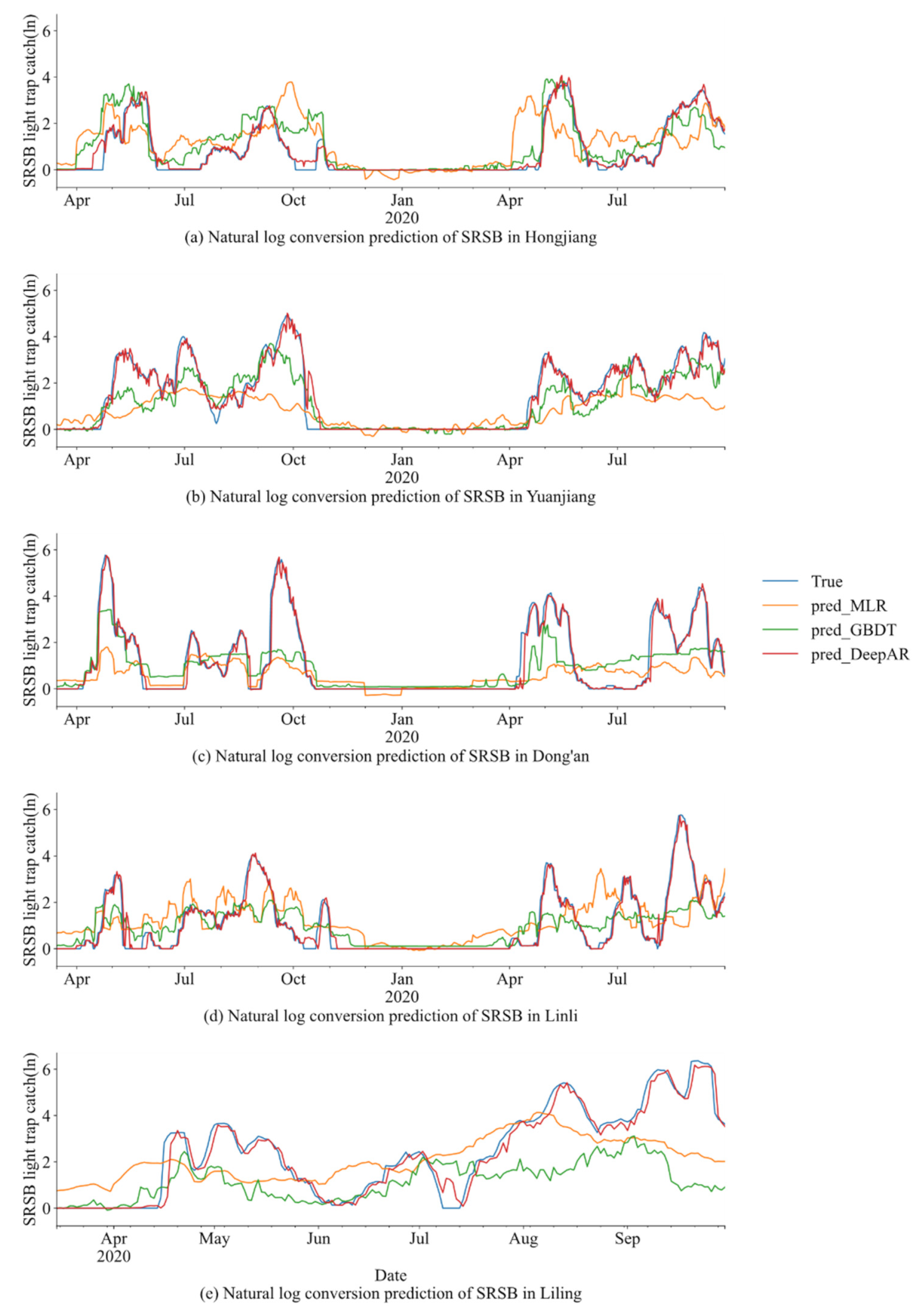
3.4. DeepAR Model Prediction

DeepAR uses the previous time step value to set the current time step of the model. These values were available within the regulatory range during training and prediction. For the prediction range, the training and the forecast values must be distinguished. During projection, time-series values within the prediction range were not available because these were the results to be predicted. Therefore, the samples from the likelihood function (whose parameters were predicted in the previous step) were used as the input values for the current time step.

Figure 4 shows the learning process of the DeepAR model [43], with the training process on the left and the prediction process on the right. After the training, the historical data $t<t_0$ were entered into the network to obtain the predicted initial hidden state $h_{i,t_0-1}{t}_0$, and then the prediction results were obtained using ancestral sampling. More specifically, at each time step, $t_0,t_0+1,\cdots ,T$ could be randomly sampled to get ${\overline{z}}_{i,t}$, the ${\overline{z}}_{i,t}$ as a partial input for the next time step. In this way, a series of all sampling values from $t_0$ to $T$ could be obtained on the time scale, and these sampling values could then be used to calculate the required target value.

The average coefficient of determination, minimum coefficient of determination, and maximum coefficient of determination of the DeepAR model based on the test dataset in the study areas (Linli, Liling, Yuanjiang, Dong’an, and Hongjiang) are ${\mathrm{R}}_{\mathrm{mean}}^2=0.952$, ${\mathrm{R}}_{\min }^2=0.945$, and ${\mathrm{R}}_{\max }^2=0.958$, respectively.

3.5. MLR, GBDT, and DeepAR Model Validation and Performance Comparison

Figure 5 compares the true and predicted values of the test datasets of the rice SRSB light trap capture after natural log transformation (ln) in different study regions under different models (traditional MLR model, machine learning GBDT, and deep learning DeepAR model).

We found that for all study regions, the MLR model could not correctly fit the actual values. Even negative predicted values were obtained for some periods (for example, in Hongjiang from December 2019 to January 2020), which have a large gap with the actual value. The GBDT model had good prediction results, although the prediction values in Hongjiang and Yuanjiang still could not accurately fit the actual values. However, the trend of the SRSB light trap catch was correctly reflected. It showed the upward and downward movement of the SRSB light trap catch in some periods (for example, in Hongjiang from April 2019 to October 2020, and in Yuanjiang from April 2019 to October 2020). The DeepAR model had the best predictions, and actual values could be accurately fitted in all study regions and periods.

The results show that the deep learning DeepAR model produced good predictions for all sites as compared to the traditional MLR model and the machine learning GBDT model.

Figure 6 shows the comparison between the light trap catch of natural log-transformed SRSB populations as predicted by the MLR, GBDT, and DeepAR models, respectively. Compared to R² and RMSE, DeepAR models produced more accurate predictions than the MLR and GBDT models, and the GBDT was more accurate than the MLR. The R² values for DeepAR, GBDT, and MLR were 0.944–0.960, 0.295–0.687, and 0.083–0.312, respectively, and the RMSE values were 0.228–0.425, 0.733–1.271, and 1.158–1.576, respectively.

Figure 7 shows the performance of MLR, GBDT, and DeepAR in evaluating the indicators MAE, RMSE, sMAPE, and R² in different study areas. We found that the MLR model showed the worst performance in the SRSB light trap catches in Hongjiang, Yuanjiang, Dong’an, and Linli. The Liling GBDT model had the worst performance, probably the smallest sample of the datasets (compared to other study regions). The DeepAR model (MAE, RMSE, sMAPE, and R² were 0.125–0.245, 0.228–0.425, 0.360–0.657, and 0.945–0.959, respectively) had the best performance in all areas, outperforming the MLR (MAE, RMSE, sMAPE, and R² were 0.856–1.297, 1.158–1.576, 0.808–1.414, and 0.083–0.312, respectively) and the GBDT (MAE, RMSE, sMAPE, and R² were 0.494–0.981, 0.733–1.271, 0.003–1.296, and 0.295–0.687, respectively) models in terms of stability and accuracy.

In conclusion, it is feasible to predict the SRSB light trap catch using the deep learning DeepAR model.

4. Discussion

Predicting pest populations helps specify pest management strategies, reduce the use of pesticides, and is an integral part of the successful implementation of IPM. For pest prediction models, weather variables such as temperature, humidity, rainfall, and sunshine duration are often used as abiotic predictors in model development [8,9,10,11,12,13,26]. We found that TEMP [1,7], RH, and SDD were positively associated with the SRSB light trap catch, while AP and PRCP were negatively associated with the SRSB light trap catch. WDSP, EVP, and MXWDSP were also associated with the SRSB light trap catch. Generally, when WDSP, EVP, and MXWDSP are moderate, the amount of SRSB is the highest.

The rice light trap was used to capture rice pests in order to study the relationship between them. We found a significant positive correlation between SRSB and RPH, and a highly significant positive correlation between SRSB and PSB. This indicates an interactional relationship between rice pests, which could be used to predict some areas with little or even no historical pest data, especially for migratory pests such as the Spodoptera odorata.

The stepwise multivariate regression model established in this study showed that the model which combined meteorological variables, associated pests, and time features (adjusted R² = 0.400) was more accurate than the model using meteorological variables alone (adjusted R² = 0.346).

The GBDT model is a suitable choice for predicting pest occurrence. Our study showed that the GBDT model produced more accurate pest predictions than the MLR model. The deep learning DeepAR model obtained the best predictions, probably because of the extended data cycles we used, and deep learning is known to perform well with large samples. Our study showed that the deep learning DeepAR model predicted the natural log-transformed SRSB light trap catch with an average accuracy of 95.2% (the average prediction accuracy of the MLR model was 16.6%, and that of the GBDT model was 50.0%), which has a good application value. Since the rice field is an open environment, the factors driving the growth of the SRSB population are variable. In addition to weather and pest-related factors, rice growth phenology, natural enemies, rice varieties, pest prevention, control information, and even farmer practices may affect population dynamics. The observed and predicted kurtosis differences in SRSB may be due to seasonality and changes in the surrounding environment. Rice-related pest factors with a larger area can be considered in future work.

5. Conclusions

In this study, we presented a prediction model for SRSB population occurrence in the Hunan Province of China by integrating time series variables of ground weather, the number of related pests captured by light traps, and the number of SRSB captured by light traps. The MLR, GBDT, and DeepAR models were constructed based on the abovementioned variables. MLR was used to study the predictive power of meteorological variables alone or combined with related pest and time variables. At the same time, the GBDT and DeepAR models were established to enhance the model prediction performance compared to MLR.

Based on the high correlation coefficient of the MLR model, the main features of the MLR model for the SRSB captured by the light trap in the research areas were selected as follows: Yuanjiang made use of AP, RPH, PSB, YSB, and Season; Hongjiang used RHmin, RPH, PSB, YSB, and Season; Dong’an used TEMP, RPH, YSB, and Season; Linli used TEMP, PSB, YSB, PLR, and Season; Liling used TEMP, PSB, YSB, PLR, and Season. The GBDT model performed better than the MLR model in four regions (Hongjiang, Yuanjiang, Dong’an, and Linli), and DeepAR performed better than MLR and GBDT in all areas.

In conclusion, deep learning-based DeepAR models can dynamically predict SRSB populations combined with the ground meteorological variables, associated pest variables, and pest variable-derived time variables, which can be applied to the timely management of crop pests after proper validation in different regions. We anticipate that these results can cooperate with an online rice pest monitoring and intelligent prediction system developed by the Hunan Provincial Department of Agriculture to support an effective early pest warning system.

References

1. Feng, Q.L. Physiology and interaction of insects with environmental factors. J. Integr. Agric. 2020, 19, 1411–1416. [Google Scholar] [CrossRef]
2. Sun, Y.; Xu, L.; Chen, Q.; Qin, W.; Huang, S.; Jiang, Y.; Qin, H. Chlorantraniliprole resistance and its biochemical and new molecular target mechanisms in laboratory and field strains of Chilo suppressalis (Walker). Pest Manag. Sci. 2018, 74, 1416–1423. [Google Scholar] [CrossRef]
3. Muralidharan, K.; Pasalu, I.C. Assessments of crop losses in rice ecosystems due to stem borer damage (Lepidoptera: Pyralidae). Crop Prot. 2006, 25, 409–417. [Google Scholar] [CrossRef]
4. Chen, M.; Shelton, A.; Ye, G. Insect-Resistant Genetically Modified Rice in China: From Research to Commercialization. Annu. Rev. Entomol. 2011, 56, 81–101. [Google Scholar] [CrossRef] [Green Version]
5. He, Y.; Zhang, J.; Gao, C.; Su, J.; Chen, J.; Shen, J. Regression analysis of dynamics of insecticide resistance in field populations of Chilo suppressalis (Lepidoptera: Crambidae) during 2002–2011 in China. J. Econ. Entomol. 2013, 106, 1832–1837. [Google Scholar] [CrossRef]
6. Wang, Y.N.; Ke, K.Q.; Li, Y.H.; Han, L.Z.; Liu, Y.M.; Hua, H.X.; Peng, Y.F. Comparison of three transgenic Bt rice lines for insecticidal protein expression and resistance against a target pest, Chilo suppressalis (Lepidoptera: Crambidae). Insect Sci. 2016, 23, 78–87. [Google Scholar] [CrossRef] [PubMed]
7. Qiang, C.K.; Du, Y.Z.; Yu, L.Y.; Qin, Y.H.; Feng, W.J. Effects of temperature stress on physiological indices of Chilo suppressalis Walker (Lepidoptera: Pyralidae) diapause larvae. Chin. J. Appl. Ecol. 2012, 23, 1365–1369. [Google Scholar]
8. Skawsang, S.; Nagai, M.; Tripathi, N.K.; Soni, P. Predicting Rice Pest Population Occurrence with Satellite-Derived Crop Phenology, Ground Meteorological Observation, and Machine Learning: A Case Study for the Central Plain of Thailand. Appl. Sci. 2019, 9, 4846. [Google Scholar] [CrossRef] [Green Version]
9. Aparecido, L.; Rolim, G.; De Moraes, J.R.D.S.; Costa, C.; Souza, P. Machine learning algorithms for forecasting the incidence of Coffea arabica pests and diseases. Int. J. Biometeorol. 2020, 64, 671–688. [Google Scholar] [CrossRef]
10. Holloway, P.; Kudenko, D.; Bell, J.R. Dynamic selection of environmental variables to improve the prediction of aphid phenology: A machine learning approach. Ecol. Indic. 2018, 88, 512–521. [Google Scholar] [CrossRef] [Green Version]
11. Narayanasamy, M.; Kennedy, J.; Geethalakshmi, V. Weather Based Pest Forewarning Model for Major Insect Pests of Rice—An Effective Way for Insect Pest Prediction. Annu. Res. Rev. Biol. 2017, 21, 1–13. [Google Scholar] [CrossRef]
12. Poggi, S.; Le Cointe, R.; Riou, J.; Larroudé, P.; Thibord, J.; Plantegenest, M. Relative influence of climate and agroenvironmental factors on wireworm damage risk in maize crops. J. Pest Sci. 2018, 91, 585–599. [Google Scholar] [CrossRef]
13. Gu, Y.H.; Yoo, S.J.; Park, C.J.; Kim, Y.H.; Park, S.K.; Kim, J.S.; Lim, J.H. BLITE-SVR: New forecasting model for late blight on potato using support-vector regression. Comput. Electron. Agric. 2016, 130, 169–176. [Google Scholar] [CrossRef]
14. Ni, T.; Zhai, J. A matrix-free smoothing algorithm for large-scale support vector machines. Inf. Sci. 2016, 358, 29–43. [Google Scholar] [CrossRef]
15. Feng, S.; Zhou, H.; Dong, H. Using deep neural network with small dataset to predict material defects. Mater. Des. 2019, 162, 300–310. [Google Scholar] [CrossRef]
16. Salman, S.; Liu, X. Overfitting Mechanism and Avoidance in Deep Neural Networks. arXiv 2019, arXiv:1901.06566. [Google Scholar]
17. Bengio, Y. Learning Deep Architectures for AI. Found. Trends Mach. Learn. 2009, 2, 1–127. [Google Scholar] [CrossRef]
18. Schmidhuber, J. Deep learning in neural networks: An overview. Neural Netw. 2015, 61, 85–117. [Google Scholar] [CrossRef] [Green Version]
19. Bengio, Y.; Courville, A.; Vincent, P. Representation Learning: A Review and New Perspectives. IEEE T. Pattern Anal. 2013, 35, 1798–1828. [Google Scholar] [CrossRef] [PubMed]
20. Deng, L.; Yu, D. Deep Learning: Methods and Applications. Found. Trends Signal Process. 2014, 7, 197–387. [Google Scholar] [CrossRef] [Green Version]
21. Lecun, Y.; Bengio, Y.; Hinton, G. Deep learning. Nature 2015, 521, 436–444. [Google Scholar] [CrossRef] [PubMed]
22. Luo, X.; Li, J.; Chen, M.; Yang, X.; Li, X. Ophthalmic Disease Detection via Deep Learning with a Novel Mixture Loss Function. IEEE J. Biomed. Health Inform. 2021, 25, 3332–3339. [Google Scholar] [CrossRef]
23. Chen, M.; Li, Y.; Luo, X.; Wang, W.; Wang, L.; Zhao, W. A Novel Human Activity Recognition Scheme for Smart Health Using Multilayer Extreme Learning Machine. IEEE Internet Things J. 2019, 6, 1410–1418. [Google Scholar] [CrossRef]
24. Sun, J.; Luo, X.; Gao, H.; Wang, W.; Gao, Y.; Yang, X. Categorizing Malware via A Word2Vec-based Temporal Convolutional Network Scheme. J. Cloud Comput. 2020, 9, 1–14. [Google Scholar] [CrossRef]
25. Luo, X.; Sun, J.K.; Wang, L.; Wang, W.P.; Zhao, W.B.; Wu, J.S.; Wang, J.H.; Zhang, Z.J. Short-Term Wind Speed Forecasting via Stacked Extreme Learning Machine With Generalized Correntropy. IEEE Trans. Ind. Inform. 2018, 14, 4963–4971. [Google Scholar] [CrossRef] [Green Version]
26. Wahyono, T.; Yaya, H.; Haryono, S.; Saleh, A.B. Enhanced lstm multivariate time series forecasting for crop pest attack prediction. ICIC Express Lett. 2020, 10, 943–949. [Google Scholar]
27. Yan, Y.; Feng, C.; Wan, M.P.; Chang, K.T. Multiple Regression and Artificial Neural Network for the Prediction of Crop Pest Risks; Springer International Publishing: Cham, Switzerland, 2015; pp. 73–84. ISBN 1865-1348. [Google Scholar]
28. Yamamura, K.; Yokozawa, M.; Nishimori, M.; Ueda, Y.; Yokosuka, T. How to analyze long-term insect population dynamics under climate change: 50-year data of three insect pests in paddy fields. Popul. Ecol. 2006, 48, 31–48. [Google Scholar] [CrossRef]
29. Ghani, I.M.M.; Ahmad, S. Stepwise Multiple Regression Method to Forecast Fish Landing. Procedia-Soc. Behav. Sci. 2010, 8, 549–554. [Google Scholar] [CrossRef] [Green Version]
30. Amiri, S.S.; Mottahedi, M.; Asadi, S. Using multiple regression analysis to develop energy consumption indicators for commercial buildings in the U.S. Energy Build. 2015, 109, 209–216. [Google Scholar] [CrossRef]
31. Friedman, J.H. Greedy Function Approximation: A Gradient Boosting Machine. Ann. Stat. 2001, 29, 1189–1232. [Google Scholar] [CrossRef]
32. Picard, R.R.; Cook, R.D. Cross-Validation of Regression Models. Publ. Am. Stat. Assoc. 1984, 79, 575–583. [Google Scholar] [CrossRef]
33. Hochreiter, S.; Schmidhuber, J. Long Short-Term Memory. Neural Comput. 1997, 9, 1735–1780. [Google Scholar] [CrossRef]
34. Hochreiter, S.; Schmidhuber, J. LSTM can solve hard long time lag problems. In Proceedings of the 9th International Conference on Neural Information Processing Systems, Denver, CO, USA, 3–5 December 1996; pp. 473–479. [Google Scholar]
35. Graves, A. Generating Sequences With Recurrent Neural Networks. arXiv 2013, arXiv:1308.0850. [Google Scholar]
36. Van den Oord, A.; Dieleman, S.; Zen, H.; Simonyan, K.; Vinyals, O.; Graves, A.; Kalchbrenner, N.; Senior, A.; Kavukcuoglu, K. WaveNet: A Generative Model for Raw Audio. arXiv 2016, arXiv:1609.03499. [Google Scholar]
37. Zaremba, W.; Sutskever, I.; Vinyals, O. Recurrent Neural Network Regularization. arXiv 2014, arXiv:1409.2329. [Google Scholar]
38. Salinas, D.; Flunkert, V.; Gasthaus, J.; Januschowski, T. DeepAR: Probabilistic forecasting with autoregressive recurrent networks. Int. J. Forecast. 2020, 36, 1181–1191. [Google Scholar] [CrossRef]
39. Draper, N.; Smith, H. Applied Regression Analysis, 2nd ed.; John Wiley: New York, NY, USA, 1981; ISBN 978-0-471-02995-3. [Google Scholar]
40. Glantz, S.A.V.; Slinker, B.K. Primer of Applied Regression and Analysis of Variance; McGraw-Hill: New York, NY, USA, 1990; ISBN 0070234078. [Google Scholar]
41. Carpenter, R.G. Principles and procedures of statistics, with special reference to the biological sciences. Eugen. Rev. 1960, 52, 172–173. [Google Scholar]
42. Chicco, D.; Warrens, M.J.; Jurman, G. The coefficient of determination R-squared is more informative than SMAPE, MAE, MAPE, MSE and RMSE in regression analysis evaluation. PeerJ Comput. Sci. 2021, 7, e623. [Google Scholar] [CrossRef]
43. Time Series Prediction—Telesens. Available online: https://www.telesens.co/2019/06/08/time-series-prediction/ (accessed on 21 September 2021).
Figure 1. The main symptom in rice of damage by SRSB.
Processes 09 02166 g001
Figure 2. Locations of study areas and light traps.
Processes 09 02166 g002
Figure 3. Variable importance derived from the GBDT model for natural log-transformed ln (SRSB) light trap catches in Yuanjiang.
Processes 09 02166 g003
Figure 4. Forecasting process of DeepAR.
Processes 09 02166 g004
Figure 5. Predicted results of the SRSB light trap catches from the test datasets using the MLR, GBDT, and DeepAR models.
Processes 09 02166 g005
Figure 6. Actual versus predicted natural log-transformed ln (SRSB) in (a) Hongjiang, (b) Yuanjiang, (c) Dong’an, (d) Linli, and (e) Liling.
Processes 09 02166 g006
Figure 7. Predicted performance of MLR, GBDT, and DeepAR in different areas.
Processes 09 02166 g007