Optimal Design and Operation of Multi-Period Water Supply Network with Multiple Water Sources

Abstract

A water supply network is an essential part of industrial and urban water systems. The water intake in a conventional water supply network varies periodically over time, depending on the amount of available water resources and the demand at water sinks or water-using units. This paper establishes a super-structural mathematical model for the optimal design and operation of a multi-period water supply network with multiple water sources. It considers the flow rate fluctuation of raw water availability and the demand of water sinks during different periods. The influence of multi-period demand variation on technology and the capacity selection of desalination water stations is examined, which affects the overall cost of the water supply network. The operating cost penalty factor is introduced, which quantitatively clarifies how the network operating status influences the operating costs. The comparison results of three scenarios considering with and without multi-period variation of water demand verify the validity of the proposed model, i.e., for a municipal water price of 4 CNY·t⁻¹ and penalty factor of 0.3, one reverse osmosis desalination unit of capacity 800 t·h⁻¹ is selected. However, in the multi-period case, two reverse osmosis desalination units with capacities of 500 t·h⁻¹ and 300 t·h⁻¹ are selected. In both cases, the operating costs are different because of the different operating status of the network. The work can guide the design and operation of industrial and urban water supply networks.

1. Introduction

Rapid socio-economic development has brought increasing pressure on natural resources, mainly on freshwater. It has been reported that the gap between supply and demand for freshwater resources and the environmental water pollution caused by wastewater discharge is becoming more and more serious [1,2,3,4]. However, implementing optimal water management methods and increasing public awareness of water conservation can reduce the overall water and supply–demand gap and wastewater discharge. Many mathematical programming-based approaches to optimize water flow rates for better water management have been proposed and successfully applied, focusing on water management in the water supply network. Moreover, along with water conservation problems, one other concern regarding the operating status of the network during seasonal variations is also crucial, which is directly linked with the technology and capacity selection of the desalination station and the economic performance of the water supply network. The operational issues regarding operational load status due to seasonal variations are ignored in previous studies and need acute attention.

Water supply network optimization, as a vital part of the industrial and urban water network, has gradually gained attention in recent years, i.e., management and scheduling of surface water and groundwater [5,6], water resource planning under uncertainty [7,8,9], and optimizing conjunctive use of surface water and groundwater [10]. However, the water supply network includes numerous water users and water resources, and water sinks vary over a specific time period. Moreover, the available amount of raw water (impure water from water resources that needs necessary pre-treatment) from different water resources also varies over a particular time. In other words, the water supply network has the characteristics of seasonal (multi-period) water demand variations. Thus, it is particularly important to study the optimal design of multi-period water supply networks.

Several researchers have focused on the optimization of multi-period networks in recent years. It is worth noting that the multi-period optimization problem has recently become a hot topic in the process system engineering area. Considerable mathematical programming models of multi-period optimization are proposed, i.e., heat integration and optimization [11,12,13], hydrogen system optimization [14,15,16], power process integration [17], and oil and gas field development [18]. Faria and Bagajewicz (2011) [19] presented a multi-period water management planning model for network integration by defining the unit capacity and mass load as optimization variables. Burgara-Montero et al. (2013) [20] considered seasonal variation and the eco-chemical response of watersheds to propose a multi-objective and multi-period optimization model. Rojas-Torreset et al. (2014) [21] proposed a multi-period mathematical model to optimize water storage planning for natural and alternative water resources’ distribution. Lira-Barragaín et al. (2016) [22] developed a multi-period water system management model for the operation and scheduling of shale gas hydraulic fracturing under uncertainty. Tosarkani and Amin (2020) [23] proposed the multi-objective robust optimization technique to design the wastewater treatment network considering multiple uncertainty sources. Note that all the research mentioned above considered the multi-period water network only within a single plant. Multi-period optimization for multiple plants has also been proposed. Boix et al. (2012) [24] introduced multi-objective optimization with, without, and shared regeneration units for eco-industrial parks considering the complexity of possible connections. Bishnu et al. (2014) [25] proposed the multi-period planning method for industrial water direct reuse within industrial cities. Arredondo-Ramírez et al. (2015) [26] developed the multi-objective mixed integer nonlinear programming (MINLP) model for collecting, storing, and distributing the water in multi-period agriculture water systems. Leong et al. (2016) [27] introduced a mathematical model based on a multi-period to fulfil system operational flexibility for chilled and cooling water networks. Liu et al. (2017) [28] proposed a multi-period water management planning model for industrial parks by considering the indirect water reuse inside multiple plants. Ang et al. (2019) [29] introduced the multi-period and multi-criterion integration method to optimize the multiple input arrangements for wastewater reuse and disposal possibilities, improving the operational costs and processing time. Pérez-Uresti et al. (2019) [30] proposed a multi-period, multi-objective model to attain the goals of identifying alternate water sources and the optimal water distribution network. The multi-period water network optimization of single and multiple plants has been extensively studied. In the literature, previous studies of multi-period water system optimization for individual plants have gained more attention and focused merely on direct inter-plant water system optimization. Furthermore, the industrial park studies only design and schedule water networks for future forecasts with new plants. All previous studies for individual plants and industrial parks use continuous freshwater intake for annualized cost estimations without specifying the water source. In comparison, the annual seasonal variations of water demand inside the single plant and industrial parks and outside water availability from resources are ignored. These shortcomings need to be appropriately addressed. It is very important to include the multi-period supply and demand fluctuations in the water supply network because this will reflect the real industrial water supply system.

As mentioned above, the water supply network has supply and demand variations in different seasons, and such a water supply network can be named a multi-period water supply network. In this study, the water supply network is made up of surface water and municipal water resources. Municipal water from the municipal distribution system is used directly to fulfill the industrial water demand. Typically, after the pre-treatment of raw water, the produced freshwater can be directly allocated to freshwater sinks, but the same freshwater needs more conditioning to produce the desalted water for desalted water sinks. The multi-period water demand fluctuations in desalted water sinks directly affect the treatment technology and design capacity selection of desalination water stations, impacting the overall cost of the water supply network. Therefore, it is necessary to analyze the optimal design of the multi-period water supply network with multiple water sources. To the best of our knowledge, there is no considerable work on the optimal design and operation of a multi-period water supply network.

To achieve an optimal water supply network design with multiple water resources, this work proposes a superstructure-based mathematical model to analyze the influence of multi-period variations in supply and demand on the water supply network. The operating cost penalty factor is included in the model, which evaluates how the operational network status affects the network operating costs. A coastal oil refinery from China is considered as a case study to illustrate the proposed approach. The case study considers three scenarios: Scenario 1 ignores the multi-period variations in the demand of water sinks with a single water resource. Scenario 1 is selected for the simple case where the water demand for all the seasons with a single resource is the same, but, as compared to the previous literature, the additional influences of penalty factors and water prices are used for the optimal technology and capacity selection. Scenario 2 includes multi-period variations in the water sinks’ demand with a single water source. Scenario 3 considers the multi-period water demand variation considering multiple water sources. Scenario 2 and scenario 3 are chosen to further check the model applicability with fluctuations in the seasonal demand and how this season demand affects the operation design of desalination units, and how it affects the total annual cost of the supply network.

2. Methodology

2.1. Problem Statement

As previously stated, the water supply network experiences seasonal variations. These variations lead to different operational loads in different periods, which directly affect the treatment technology and capacity selection of desalination stations, impacting the overall cost of the water supply network. This section presents a superstructure for optimal technology and capacity selection of desalination station under seasonal variations. The general superstructure of the proposed multi-period water supply network is shown in Figure 1. For a given set of water resources $(r\in N_r)$, the corresponding water pre-treatment systems (RWTS) are available. Each water resource has different water properties and unit prices. A set of water properties $(p\in N_p$, i.e., conductivity, turbidity, and chemical oxygen demand COD) is defined to specify the water quality. Three water users $(k\in N_k$, i.e., freshwater user, desalted water user, and wastewater treatment system) are defined as water sinks. After the raw water is processed through a raw water pre-treatment system (RWTS) (i.e., flocculation, filtration, pH adjustment, carbon dioxide adsorption) to meet water property requirements of freshwater, part of freshwater is sent to the freshwater users, and the other part is directed to the desalination station for further treatment to produce desalted water. The residual water from the raw water pre-treatment and desalination stations is sent to the wastewater treatment system for further treatment. It is worth noting that in the proposed superstructure, residual water allocation is represented by brown streams. In contrast, all other types of water, such as raw water, freshwater, and desalted water, are shown by black streams.

Freshwater tank (FWT) and desalted water tank (DWT) are stated as a set $(s\in N_s)$ to facilitate water storage and distribution. Considering seasonal variations in the desalted water demand, different processing techniques, production scheduling, and different desalted water station capacity specifications are available.

All the desalination treatment technologies have different treatment performance, water production ratios, and operational costs at different operational loads, affecting the total annual cost of the supply network under demand variations. Based on the proposed superstructure, this work aims to optimize the technology and capacity selection of water supply network design, considering multi-period demand variations to reduce overall annualized costs.

2.2. Mathematical Model

A mathematical model for the optimal design of multi-period water supply network with multiple water sources based on the proposed superstructure (see Figure 1) and the problem statement is presented. A list of indices, sets, parameters, and variables are presented in the notation section, where all the parameters are denoted as upper-case symbols, and all the variables are denoted as lower-case symbols.

2.3. Constraints

The maximum amount of raw water available from different types of water resources varies in different seasons. For example, the available amount of surface water is greatly affected by the seasonal changes, so the raw water supplied from each water resource in different time periods cannot exceed the maximum supply limit, as shown in Equation (1)

$$f_{r,t}={\mathrm{F}}_{r,t}^{\max }\forall r\in N_r,t\in N_t$$

(1)

where $f_{r,t}$ is the flowrate from raw water resources in different time periods. ${\mathrm{F}}_{r,t}^{\max }$ denotes the maximum flowrate of raw water available in different time periods. A traditional water supply network in a coastal area can use municipal water, surface water, groundwater, municipal treated wastewater, and seawater as raw water resources. However, in many cities, municipal treated wastewater is used to irrigate the public parks and green belts along the roads. In some areas, groundwater usage as a water resource is strictly limited to ensure an adequate level of clean water underground. The use of seawater as a raw water resource is costly because the pre-treatment technologies related to seawater desalination are expensive and still in the developing status. Thus, to simplify the problem, this study only considers municipal water (MW) and surface water (SFW) as raw water resources. There are no limitations involved regarding this simplification. It is only introduced to reduce the size of the model. This model can be used for other water resources, such as seawater or municipal treated wastewater, as raw water sources, but the mathematical model needs to include the relevant pre-treatment systems for additional water resources.

The municipal water properties meet the industrial freshwater demand standards, and it can be directly supplied to the freshwater tank (FWT), as shown in Equation (2).

$$f_{r,t}=f_{r,s,t}\forall r=MW,s=FWT,t\in N_t$$

(2)

where $f_{r,s,t}$ is the flowrate from water resource r to water storage tank s during the different time periods t. Surface water generally comes from rivers, lakes, and reservoirs. The surface water properties cannot meet the industrial freshwater standards, so it must be treated by the raw water pre-treatment system (i.e., flocculation, filtration, pH adjustment, carbon dioxide adsorption), as expressed in Equation (3).

$$f_{r,t}=f_{r,pt,t}\forall r=SFW,pt=RWTS,t\in N_t$$

(3)

where $f_{r,pt,t}$ is the flowrate from water resource r to raw water pre-treatment unit pt during different time periods t.

In this paper, the raw water pre-treatment system is simplified to a fixed water production rate and removal ratio units. In the pre-treatment system, each unit removes the impurities present in the raw water. The inlet water stream goes into the unit with high property concentration, and two steams come out, namely the product water and residual water. The removal ratio is used to relate the inlet and outlet properties. The production ratio is used to relate the inlet and outlet flow rates. However, in actual pre-treatment units, some other characteristics are also involved, such as energy consumption, chemical input, and unit maintenance. Therefore, to simplify the mathematical formulation, we only use the removal ratio and production ratio to relate inlet and outlet properties and flowrate, ignoring the other characteristics. The properties of product water depend on the efficiency of pre-treatment system and quality of inlet raw water. Different properties (i.e., turbidity, conductivity, COD) are used to specify the streams. A property operator $\psi$ is introduced to calculate the property balance consistent with the pollutant concentration balance calculation. The property operator in this paper is valid to the first rule [31,32], which is used to transfer the non-equilibrium properties and can be expressed by Equation (4). Equations (5) and (6) express the inlet and outlet flowrate balance of raw water pre-treatment system (RWTS), and Equation (7) represents the property balance relationship.

$$\psi (p)=p\forall p\in \left\{\mathrm{Turbidity},\mathrm{Conduvtivity},\mathrm{COD}\right\}$$

(4)

$$f_{pt,t}^{in}=f_{pt,t}^{prod}+f_{pt,t}^{resd}\forall pt=RWTS,t\in N_t$$

(5)

$$f_{pt,t}^{prod}=A_{pt}·f_{pt,t}^{in}\forall pt=RWTS,t\in N_t$$

(6)

$${\psi }_{pt,p,t}^{in}·f_{pt,t}^{in}={\psi }_{pt,p,t}^{prod}·f_{pt,t}^{prod}+{\psi }_{pt,p,t}^{resd}·f_{pt,t}^{resd}\forall pt=RWTS,p\in N_p,t\in N_t$$

(7)

where $f_{pt,t}^{in}$ is the inlet flowrate of the pre-treatment system. $f_{pt,t}^{prod},f_{pt,t}^{resd}$ represent the flowrate of product water and residue water, respectively. $A_{pt}$ denotes the water production ratio. ${\psi }_{pt,p,t}^{in},{\psi }_{pt,p,t}^{prod},{\psi }_{pt,p,t}^{resd}$ represent the property operator values of inlet water, product water, and residue water, respectively.

The properties of product water are linked to the properties of inlet water and the efficiency of pre-treatment system. The property operator value for product water can be calculated, as shown in Equation (8).

$${\psi }_{pt,p,t}^{prod}=H_{pt}(f_{pt,t}^{in}.{\psi }_{pt,p,t}^{in})\forall pt=RWTS,p\in N_p,t\in N_t$$

(8)

where $H_{pt}$ denotes the efficiency of the pre-treatment system. The storage tanks are mainly set up to safeguard the water flowrate variation in supply and demand during different time periods. The freshwater tank (FWT) can accept municipal water or product water from RWTS if it meets the freshwater property value limits. The inlet water flowrate and property balance of FWT are shown in Equations (9) and (10).

$$f_{s,t}^{in}=\underset{pt=RWTS}{f_{{}_{pt,t}}^{prod}}+\underset{r=MW}{f_{{}_{r,s,t}}^{}}\forall s=FWT,t=N_t$$

(9)

$$f_{s,t}^{in}·{\psi }_{s,p,t}^{in}=\underset{pt=RWTS}{f_{pt,t}^{prod}·{\psi }_{pt,p,t}^{prod}}+\underset{r=MW}{f_{r,s,t}^{}·{\mathsf{\psi }}_{r,p,t}^{}}\forall s=FWT,p\in N_p,t=N_t$$

(10)

where $f_{s,t}^{in}$ is the inlet flowrate of the storage tank. ${\psi }_{s,p,t}^{in}$ denotes the property operator value at the inlet of the storage tank during different time periods. The water from a freshwater tank can be directed to different freshwater users. For instance, it is used as makeup water in the circulating water station, can be sent to the desalinated water station, and other production processes. This article only considers the desalinated water station and the freshwater users as freshwater sinks. The outlet flowrate balance of the freshwater tank is shown in Equation (11).

$$f_{s,t}^{out}=\underset{}{f_{s,k,t}^{}}+{\displaystyle \sum _{dt\in N_{dt}}{f}_{s,dt,t}}\forall s=FWT,t=N_t$$

(11)

where is the outlet flowrate from the storage tank. $f_{s,k,t}^{}$ denotes the flowrate from freshwater storage tank s to water sink k. $f_{s,dt,t}$ is the flowrate from freshwater storage tank s to desalination unit dt. The inlet water flowrate and property operator intake value of the desalination unit are shown in Equations (12) and (13), respecrespectively.

$$f_{dt,t}^{in}=\underset{s=FWT}{f_{s,dt,t}}\forall dt\in N_{dt},t\in N_t.$$

(12)

$${\psi }_{dt,p,t}^{in}=\underset{s=FWT}{{\psi }_{s,p,t}^{out}}\forall dt\in N_{dt},p\in N_p,t\in N_t$$

(13)

where $f_{dt,t}^{in}$ is the inlet flowrate of the desalination unit. The outlet property operator value of the freshwater tank (FWT) is equal to the inlet property operator value of desalination unit. The inlet water flowrate of raw water pre-treatment and desalination units cannot exceed the 90% of design treatment capacity, expressed in Equations (14) and (15), respectively.

$$f_{pt,t}^{in}\le 0.9·CA{P}_{pt}^{}=F_{pt}^{\max ,in}\forall pt=RWTS,t\in N_t$$

(14)

$$f_{dt,t}^{in}\le 0.9·CA{P}_{dt}^{}=F_{dt}^{\max ,in}\forall dt\in N_{dt},t\in N_t$$

(15)

where $F_{pt}^{\max ,in},F_{dt}^{\max ,in}$ represent the maximum inlet flowrate of the pre-treatment system and desalination unit, respectively. $f_{pt,t}^{in},f_{dt,t}^{in}$ denote the inlet flowrate of the pre-treatment system and desalination unit during different time periods, respectively.

To meet the specific demand, different desalination units may be employed in different time periods, as shown in Equation (16).

$$f_{dt,t}^{in}\le F_{dt}^{\max ,in}·y_{dt,t}^{}\forall dt\in N_{dt},t\in N_t$$

(16)

where $y_{dt,t}^{}$ denotes the binary variable for operational status of desalination unit. It is equal to zero when desalination does not work, and the desalination unit is operational when $y_{dt,t}^{}$ is equal to one. The product water from the desalination unit is sent to the desalted water tank (DWT), the outlet water flowrate balance is expressed by

$$f_{dt,t}^{prod}=\underset{s=DWT}{f_{dt,s,t}}\forall dt\in N_{dt},t\in N_t$$

(17)

where $f_{dt,s,t}$ denotes the desalted water flowrate from desalination unit dt to the desalted water tank (DWT) during different time periods t. The desalted water from the DWT is sent to the desalted water sinks, and the outlet water flowrate balance is expressed by Equation (18).

$$f_{s,t}^{out}=\underset{}{f_{s,k,t}^{}}\forall s=DWT,t=N_t$$

(18)

where $f_{s,k,t}^{}$ denotes the flowrate from the desalted water tank to the desalted water sink during different time periods. The inlet flowrate and property operator value of each sink must meet the requirements expressed in Equations (19) and (20).

$$F_{k,t}^{\min }\le f_{k,t}^{in}\le F_{k,t}^{\max }\forall k\in N_k,t\in N_t$$

(19)

$${\psi }_{k,p,t}^{\min }\le {\psi }_{k,p,t}^{in}\le {\psi }_{k,p,t}^{\max }\forall k\in N_k,p\in N_p,t\in N_t$$

(20)

where $F_{k,t}^{\min },F_{k,t}^{\max }$ are the minimum and maximum flowrate demand of desalted water sinks, respectively, and ${\psi }_{k,p,t}^{\min },{\psi }_{k,p,t}^{\max }$ represent the minimum and maximum property operator value of desalted water sinks, respectively.

The residual water from the desalination unit and RWTS can be sent to the wastewater treatment system for further treatment to meet the environmental discharge regulations. The inlet flowrate and property balance of wastewater treatment can be expressed by

$$f_{k,t}^{in}=\underset{pt=RWTS}{f_{pt,k,t}^{resd}}+{\displaystyle \sum _{dt}{f}_{dt,k,t}^{resd}}\forall k=WTS,t\in N_t$$

(21)

$$f_{k,t}^{in}·{\psi }_{k,p,t}^{in}=\underset{pt=RWTS}{f_{pt,k,t}^{resd}·{\psi }_{pt,p,t}^{resd}}+{\displaystyle \sum _{dt}{f}_{dt,k,t}^{resd}·{\psi }_{dt,p,t}^{resd}}\forall k=WTS,p\in N_p,t\in N_t$$

(22)

where $f_{pt,k,t}^{resd},f_{dt,k,t}^{resd}$ are the flowrate from pre-treatment unit pt and desalination unit dt, respectively, to the wastewater pre-treatment system, which is stated as water sink k.

2.4. Objective Function

The objective function is to minimize the total annualized cost (TAC) of the water supply network, which mainly includes the raw water resources cost, wastewater treatment cost, the investment and operating costs of RWTS, and desalination water station. The objective function can be expressed by,

$$\begin{array}{ll}OBJ\min TAC=& {\displaystyle \sum _{t\in N_t}{\displaystyle \sum _{r\in N_r}C{W}_r·f_{r,t}}·\Delta t_t}+{\displaystyle \sum _{t\in N_t}C{W}_{resd}^{}·\underset{k=WTS}{f_{k,t}^{in}}·\Delta t_t}+{\displaystyle \sum _{t\in N_t}EO{C}_{pt}·f_{pt,t}^{in}·\Delta t_t}\\ & \underset{pt=RWTS}{+Af·\left[(1+P{R}_{pt})·EI{C}_{pt}·{(V_{pt}^{CAP})}^{\beta }·y_{pt}\right]}\\ & +{\displaystyle \sum _{t\in N_t}{\displaystyle \sum _{dt\in N_{dt}}\left(EO{C}_{dt,t}^{Based}+EO{C}_{dt,t}^{Penalty}\right)·f_{dt,t}^{in}}·\Delta t_t}\\ & +{\displaystyle \sum _{dt\in N_{dt}}Af·\left[(1+P{R}_{dt})·EI{C}_{dt}·{(V_{dt}^{CAP})}^{\beta }·y_{dt}\right]}\end{array}$$

(23)

where $C{W}_r^{}$ is the per ton cost of the raw water. $C{W}_{resd}^{}$ denotes the per ton treatment cost of the residual water. $\Delta t_t$ is the time length in minutes. $Af$ denotes the annual factor. $EO{C}_{pt}$ is the per ton operating cost of the pre-treatment system. $EI{C}_{pt}^{},EI{C}_{dt}^{}$ are the investment cost of the pre-treatment system and desalination water station, respectively. $P{R}_{pt}^{},P{R}_{dt}^{}$ are the installation costs of pre-treatment system and desalted water station as a percentage of total investment cost, respectively. ${(V_{pt}^{CAP})}^{\beta },{(V_{dt}^{CAP})}^{\beta }$ represent the storage tank capacities in which $\beta$ is the depreciation factor. $y_{pt},y_{dt}$ denote the binary variables for the operational status of the pre-treatment system and desalination water station, respectively.

When the desalination is under partial load condition, the operation cost per unit of feed water is slightly higher than that under full load conditions. We propose to use the unit penalty cost to describe this feature and use the penalty factor, the ratio of feed water flowrate to maximum value, and the basic unit operating cost to calculate this additional penalty operating cost as shown in Equation (24).

$$EO{C}_{dt,t}^{Penalty}={\alpha }^{Penalty}·EO{C}_{dt}^{based}·(1-\frac{f_{dt,t}^{in}}{F_{dt}^{\max ,in}})\forall dt\in N_{dt},t\in N_t$$

(24)

where $EO{C}_{dt,t}^{Penalty}$ represents the per ton operating penalty cost of the desalination unit and ${\alpha }^{Penalty}$ is the penalty factor. $EO{C}_{dt}^{based}$ is the basic operational cost of the desalination unit, which means the per ton operating cost of desalination (i.e., 4.75 CNY·t⁻¹ for IX and 2.84 CNY·t⁻¹ for RO in

Table 1. Parameters related to desalination technologies.

Item	IX	RO
Investment economy scale factor	0.85
Annual factor of investment costs	0.094
PR (%)	40	25
Cost factor IC (104 CNY)	14.77	7.74
Water production ratio	0.9	0.7
Conductivity removal rate	0.995	0.998
Turbidity removal rate	0	0.99
COD removal rate	0	0.9
Rated ton water treatment cost (CNY·t−1)	4.75	2.84
Available treatment capacities (t·h−1)	250, 400, 600	300, 500, 800

when running at full load state. In addition, if the water treatment unit is used in a certain period, the investment cost is considered; otherwise, the investment cost is not considered. This constraint is expressed by Equations (25) and (26).

$$y_{dt}^{}\ge \frac{{\displaystyle \sum _t{y}_{dt,t}^{}}}{M}\forall dt\in N_{dt}$$

(25)

$$y_{pt}^{}\ge \frac{{\displaystyle \sum _t{y}_{pt,t}^{}}}{M}\forall pt=RWTS$$

(26)

2.5. Model Summary

Model P—Total annualized cost (TAC) is the objective function.

min TAC is given in Equation (23).

s.t.

mass balance constraints (1)–(3), (5), (6) (9), (11), (12), (17), (18), (21).

cost constraints (24).

property balance constraints (4), (7), (8), (10), (13) (22).

boundary constraint (19), (20).

capacity constraints for storage tank s (18), (19).

logical constraint (14), (15), (25), (26).

Note that binary variables and nonlinear relations (i.e., $f_{k,t}^{in}·{\psi }_{k,p,t}^{in}$) are included in the model P; therefore, the model belongs to a mixed integer nonlinear programming (MINLP) problem. It is solved in GAMS software using BARON solver (based on the PC condition: Intel^® Core^TM i5-3330 3.2 GHz and 4.00 GB RAM, operating Windows 10, 64-bit operating system, GAMS software version is 24.2.3). The absolute optimality acceptance of all solvers is established as 10⁻⁶.

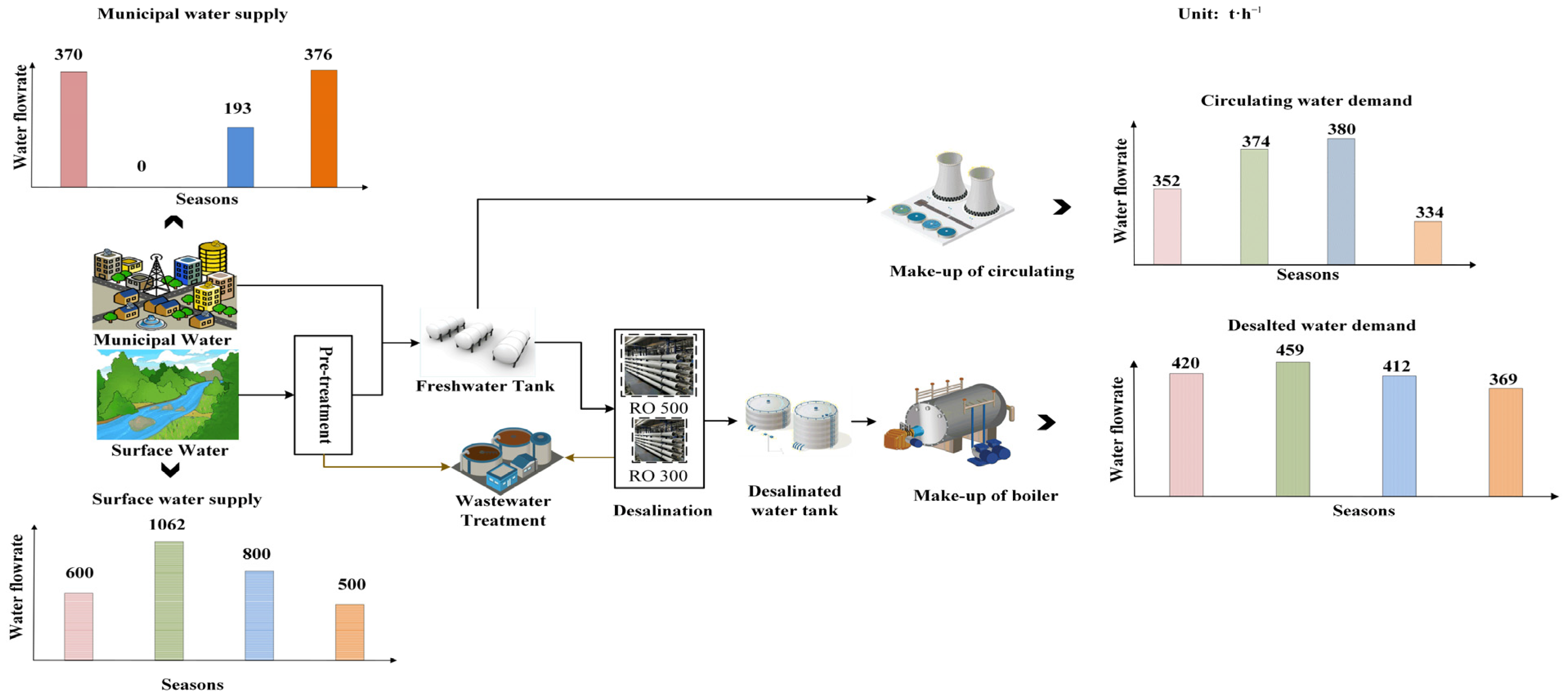
2.6. Case Description

A coastal oil refinery water supply network is selected as a case study to implement the proposed MINLP model. To attain sustainable industrial development, all the typical industrial water networks are striving to improve water management, and chosen case study is one of them. The present case is a perfect example concerning the seasonal fluctuations in water supply and demand with multiple water resources. This methodology can easily be adapted for other industrial cases. The raw available water resources to fulfill the water demand include surface water and municipal water. Considering the effect of seasonal rainfall and surface water demand from other water consumers, the maximum available amount of surface water in different seasons is different. The municipal water supply comes from the city waterworks and provides a high-quality and stable water supply. This paper takes turbidity, conductivity, and COD as the primary water properties and these are used to characterize the water quality instead of contaminants. Different parameters associated with desalination technologies are shown in Table 1. There are two kinds of technologies selected for the desalination station: ion exchange (IX) and reverse osmosis (RO). The treatment capacities of the two technologies include large, medium, and small specifications. The cost of wastewater treatment is 0.33 CNY·t⁻¹, the water pre-treatment cost of RWTS is 0.28 CNY·t⁻¹, the investment cost coefficient is CNY 7000, and the annualized duration is 8000 h.

Municipal water can provide a continuous and stable water supply coming from a municipal water plant, and the water required by the water sink can be completely supplied by municipal water as a single resource. The amount of surface water available is minimum in the fourth season, while it is maximum in the second season. In different seasons, the demand for freshwater, desalted water, and the maximum available water from different water sources are shown in

Table 2. Water demand and water source availability in different seasons.

Season	First	Second	Third	Fourth	Mean
Minimum demand of desalted water (t·h−1)	420	459	412	369	415
Minimum demand of circulating water (t·h−1)	352	374	380	334	360
Maximum supply of municipal water (t·h−1)	-	-	-	-	-
Maximum supply of surface water (t·h−1)	600	1500	800	500	925

. Freshwater demand is the makeup water of circulating water. The demand for desalted water and circulating water makeup is low in the fourth season, and it is high in the second season. Note that the maximum flowrate from municipal water supply is not restricted. The maximum supply of municipal water is represented by (-) in Table 2, indicating that it can provide any flowrate in the corresponding season.

Table 3. Properties of the water resource, freshwater, and desalted water.

Properties	MW	SFW	FW	DW
			Upper Bound	Upper Bound
Turbidity/(NTU)	1	7	3	1
Conductivity/μs·cm−1	450	590	1000	5
COD/(mg·L−1)	2	12	5	5

shows the properties of both water resources and required upper bounds. The property operator value for inlet water and product water of the pre-treatment unit is shown in Equation (27).

$$f^{prod}·{\psi }_p^{prod}=(1-R_p)·f^{in}·{\psi }_p^{in}\forall p\in N_p$$

(27)

We analyzed three scenarios to illustrate the influence of multi-period variations and multiple water sources on the water supply network design. Scenario 1: assume that the water supply network uses a single water source, and the water demand for the system does not change with time. The demand for water in the water supply network is the mean value of four seasons. In Scenario 2, the water supply network uses a single water source, and the water demand changes periodically. Scenario 3 considers the optimal design of a multi-period water supply network with multiple water resources and, simultaneously, analyzes the influence of crucial parameter changes on the supply network optimization.

3. Result and Discussion

3.1. Scenario 1—Ignoring Multi-Period Changes in Water Flowrate

In Scenario 1, the freshwater and desalted water sinks’ demand is constant; namely, the desalted water and circulating makeup water demands are 415 t·h⁻¹ and 360 t·h⁻¹, respectively. The water resource is only municipal water. As the municipal water fulfills the quality requirements of the freshwater consumers, it can directly go to freshwater water sinks from the freshwater tank. To produce the desalted water from freshwater, it needs further treatment in a desalination station. We perform the sensitivity analysis of the water price and penalty factor at the partial load operation of the desalination station per ton of water processed on the optimal operational water supply network design. When the municipal water is 4 CNY·t⁻¹, the penalty factor per ton of water cost at partial load operation is 0 (basic scenario). The optimal water supply network is shown in Figure 2, and the total annualized cost distribution is shown in Figure 3.

Figure 2 shows that, when the municipal water price is 4 CNY·t⁻¹, and the penalty factor is 0, we use a reverse osmosis-based unit with a water capacity of 800 t·h⁻¹ as a desalination water station. The total annualized cost is 47.1 million CNY·y⁻¹. As shown in Figure 3, the total cost of municipal water accounts for 65%, the operational and investment costs of the desalination unit account for 28% and 6%, respectively, and the cost of the wastewater treatment system only accounts for 1%. When the municipal water price is 4 CNY·t⁻¹, the influences of different penalty factors (step size 0.1) on technology and the capacity selection of the desalination water station and water supply network optimization are shown in

Table 4. Optimal operation scheme under different penalty factors (Scenario 1).

Penalty Factor α	0–0.3
Technology, design capacity (t·h−1)	Period	T1	T2	T3	T4
RO, 800	Actual intake (t·h−1)	592.86	592.86	592.86	592.86
Penalty factor α	0.4–0.9
Technology, design capacity (t·h−1)	Period	T1	T2	T3	T4
RO, 500	Actual intake (t·h−1)	450	450	450	450
RO, 300		142.86	142.86	142.86	142.86
Penalty factor α	≥1.0
Technology, design capacity (t·h−1)	Period	T1	T2	T3	T4
RO, 300	Actual intake (t·h−1)	270	270	270	270
RO, 300		270	270	270	270
RO, 300		52.86	52.86	52.86	52.86

.

Table 4 shows the optimal operation scheme under different penalty factors for scenario 1. Considering the technology and capacity selection, with a penalty factor of less than 0.3, we use one RO unit with a water capacity of 800 t·h⁻¹ as a desalination water station. When the penalty factor is more than 0.4 and less than 0.9, we use two RO units with capacities of 500 t·h⁻¹ and 300 t·h⁻¹ as a desalination water station. The unit with a water capacity of 500 t·h⁻¹ operates at full load, and the other operates at partial load. When the penalty factor is equal to or greater than 1, we use three RO units with capacities of 300 t·h⁻¹ as a desalination water station, two of them operate at full load, and one operates at partial load. Different types of cost comparison before and after optimization, with and without considering the technology and capacity selection for the desalination unit, are shown in Figure 4. The trends considering the technology and capacity selection are defined as optimal results. Figure 4 shows that the penalty factor equal and below 0.3 does not affect the operational penalty cost, investment cost, and total cost of the desalination station. Figure 4a shows the impact of the penalty factor on operating penalty costs. Figure 4b shows the impact of the penalty factor on the investment cost of the desalination water station. Figure 4c shows that with the increase in penalty factor, the total cost of multiple small capacity units is less than that of one large capacity unit, such as when the penalty factor is 1. The total cost of the latter is 60.32 × 10⁴ CNY·y⁻¹ more than the former.

We also analyzed the influences of changing the municipal water prices on total annualized cost, operating cost, investment cost, operating penalty cost, and wastewater treatment cost of desalination unit for a single time period. The comparison of different costs before and after the optimization, with and without considering the technology and capacity selection for changing municipal water prices, are shown in Figure 5. For a penalty factor of 0.5, the influences of different municipal water prices on the technology and capacity selection of desalination water stations in a single time period are shown in

Table 5. Optimal operation scheme under different water price (Scenario 1).

Municipal Water Price (CNY·t−1)	4–5
Technology, design capacity (t·h−1)	Period	T1	T2	T3	T4
RO, 500	Actual intake (t·h−1)	450	450	450	450
RO, 300		142.86	142.86	142.86	142.86
Municipal water price (CNY·t−1)	6–10
Technology, design capacity (t·h−1)	Period	T1	T2	T3	T4
IX, 250	Actual intake (t·h−1)	225	225	225	225
IX, 250		225	225	225	225
RO, 300		14.29	14.29	14.29	14.29
Municipal water price (CNY·t−1)	≥11
Technology, design capacity (t·h−1)	Period	T1	T2	T3	T4
IX, 600	Actual intake (t·h−1)	461.11	461.11	461.11	461.11

.

As shown in Table 5, when the municipal water price is less than 5 CNY·t⁻¹, we use two RO units with water capacities of 500 t·h⁻¹ and 300 t·h⁻¹. The unit with a water capacity of 500 t·h⁻¹ operates at full load, while the other operates at partial load. When the municipal water price is more than 6 CNY·t⁻¹ and less than 10 CNY·t⁻¹, we use two IX units with water capacities of 250 t·h⁻¹, which operate at full load, and one RO unit with a water capacity of 300 t·h⁻¹ operating at partial load. When the municipal water price is 11 CNY·t⁻¹, we use one IX unit with a water capacity of 600 t·h⁻¹.

For the municipal water price of 6 CNY·t⁻¹, Figure 5 shows that the total annualized cost is reduced by 71.17 × 10⁴ CNY·y⁻¹ for optimal results, but the operating cost and investment cost are increased by 245.52 × 10⁴ CNY·y⁻¹ and 395.49 × 10⁴ CNY·y⁻¹, respectively. The operating penalty cost and wastewater treatment cost are reduced by 61.05 × 10⁴ CNY·y⁻¹ and 33.94 × 10⁴ CNY·y⁻¹, respectively. Similarly, when the municipal water price is 11 CNY·t⁻¹, the total annualized cost is reduced by 585.56 × 10⁴ CNY·y⁻¹ for optimal results. The operating cost, investment cost, and operating penalty cost are increased by 405.25 × 10⁴ CNY·y⁻¹, 151.76 × 10⁴ CNY·y⁻¹, and 51.57 × 10⁴ CNY·y⁻¹, respectively, while the wastewater treatment cost is reduced by 34.78 × 10⁴ CNY·y⁻¹. The results show that when the water price is low, it is more economical to use the RO units for desalination. With the increasing water price, it is more economical to use the IX device for desalination.

3.2. Scenario 2—Considering Multi-Period Changes in Water Flowrate

In this section, we optimize the water supply network with multi-period changes in water demand with a single water resource and study the impact of key parameter changes on optimizing the multi-period water supply network. For the municipal water price of 4 CNY·t⁻¹, the impacts of different penalty factors (step size 0.1) on the technology and capacity selection of the desalination water station and water supply network optimization are shown in

Table 6. Optimal operation scheme under different penalty factors (Scenario 2).

Penalty Factor α	0–0.2
Technology, design capacity (t·h−1)	Period	T1	T2	T3	T4
RO, 800	Actual intake (t·h−1)	600	655.71	588.57	527.14
Penalty factor α	0.3–1.2
Technology, design capacity (t·h−1)	Period	T1	T2	T3	T4
RO, 500	Actual intake (t·h−1)	450	450	450	450
RO, 300		150	205.71	138.57	77.14
Penalty factor α	≥1.3
Technology, design capacity (t·h−1)	Period	T1	T2	T3	T4
RO, 300	Actual intake (t·h−1)	270	270	270	270
RO, 300		270	270	270	270
RO, 300		60	115.71	48.57	0

. When the penalty factor is less than 0.3, we use one RO device with a water capacity of 800 t·h⁻¹ as a desalination water station. In the multi-period scenario, the water intake varies in different time periods for the same design capacity of the desalination unit; for example, the water intake is 600 t·h⁻¹ in time period T1 and 655.71 t·h⁻¹ in time period T2. When the penalty factor is more than 0.3 and less than 1.2, we use two RO units: with water capacities of 500 t·h⁻¹ and 300 t·h⁻¹ as a desalination water station, the unit with a water capacity of 500 t·h⁻¹ operates at full load, and the other operates at partial load. When the penalty factor is more than or equal to 1.3, we use three RO devices, each of water capacity 300 t·h⁻¹, as a desalination water station, two of them operate at full load, while one operates at partial load. Note that the RO unit that operates at a partial load does not operate in time period T4. By comparing the sensitivity analysis results of Table 4 (Scenario 1) and Table 6 (Scenario 2), it is found that in both scenarios, when the penalty factor changes, it influences the capacity selection of desalination stations. With the increasing penalty factor, it is more economical to use multiple units with small capacity. Furthermore, the optimal operational scheme with a penalty factor of 0.4–0.9 in a single period corresponds to a penalty factor of 0.3–1.2 in a multi-period. For instance, for penalty factor 0.3 in scenario 1, an RO with a capacity of 800 t·h⁻¹ is selected, while scenario 2 selects two ROs with capacities of 500 t·h⁻¹ and 300 t·h⁻¹. Similarly, the operational scheme of three ROs, each with a capacity of 300 t·h⁻¹, is employed in a single period for a penalty factor equal and above 1, while for a multi-period, this operational scheme is adopted for a penalty factor equal and above 1.2.

The influence of water price changes in scenario 2 on the technology and capacity selection of the desalination water station and water supply network optimization are shown in

Table 7. Optimal operation scheme under different water price (Scenario 2).

Municipal Water Price (CNY·t−1)	4–5
Technology, design capacity (t·h−1)	Period	T1	T2	T3	T4
RO, 500	Treatment capacity (t·h−1)	450	450	450	450
RO, 300		150	205.71	138.57	77.14
Municipal water price (CNY·t−1)	6
Technology, design capacity (t·h−1)	Period	T1	T2	T3	T4
IX, 400	Treatment capacity (t·h−1)	360	360	360	360
RO, 300		137.14	192.86	125.71	64.29
Municipal water price (CNY·t−1)	≥7
Technology, design capacity (t·h−1)	Period	T1	T2	T3	T4
IX, 600	Treatment capacity (t·h−1)	466.67	510	457.78	410

. When the penalty factor is 0.5, and the municipal water price is less than 5 CNY·t⁻¹, we use two RO units with 500 t·h⁻¹ and 300 t·h⁻¹ capacities as a desalination water station. The unit with a water capacity of 500 t·h⁻¹ operates at full load, while the other operates at partial load. When the municipal water price is less than 6 CNY·t⁻¹, we use one IX unit of 400 t·h⁻¹ to operate at full load and one RO unit with 300 t·h⁻¹ to operate at partial load. When the municipal water price is more than or equal to 7 CNY·t⁻¹, we use only one IX unit with a water capacity of 600 t·h⁻¹. The results of Table 5 and Table 7 show that water price changes in both scenarios influence the technology and capacity selection. For example, at the municipal water price of 6 CNY·t⁻¹, we use one IX unit with 400 t·h⁻¹ under a multi-period scenario but need two IX units with a capacity of 300 t·h⁻¹ under the single period scenario. For the municipal water price of 7 CNY·t⁻¹, we use one IX unit of capacity 600 t·h⁻¹ under the multi-period scenario, while in the case of a single period, we need to use one IX unit of capacity 600 t·h⁻¹ when the water price is 11 CNY·t⁻¹.

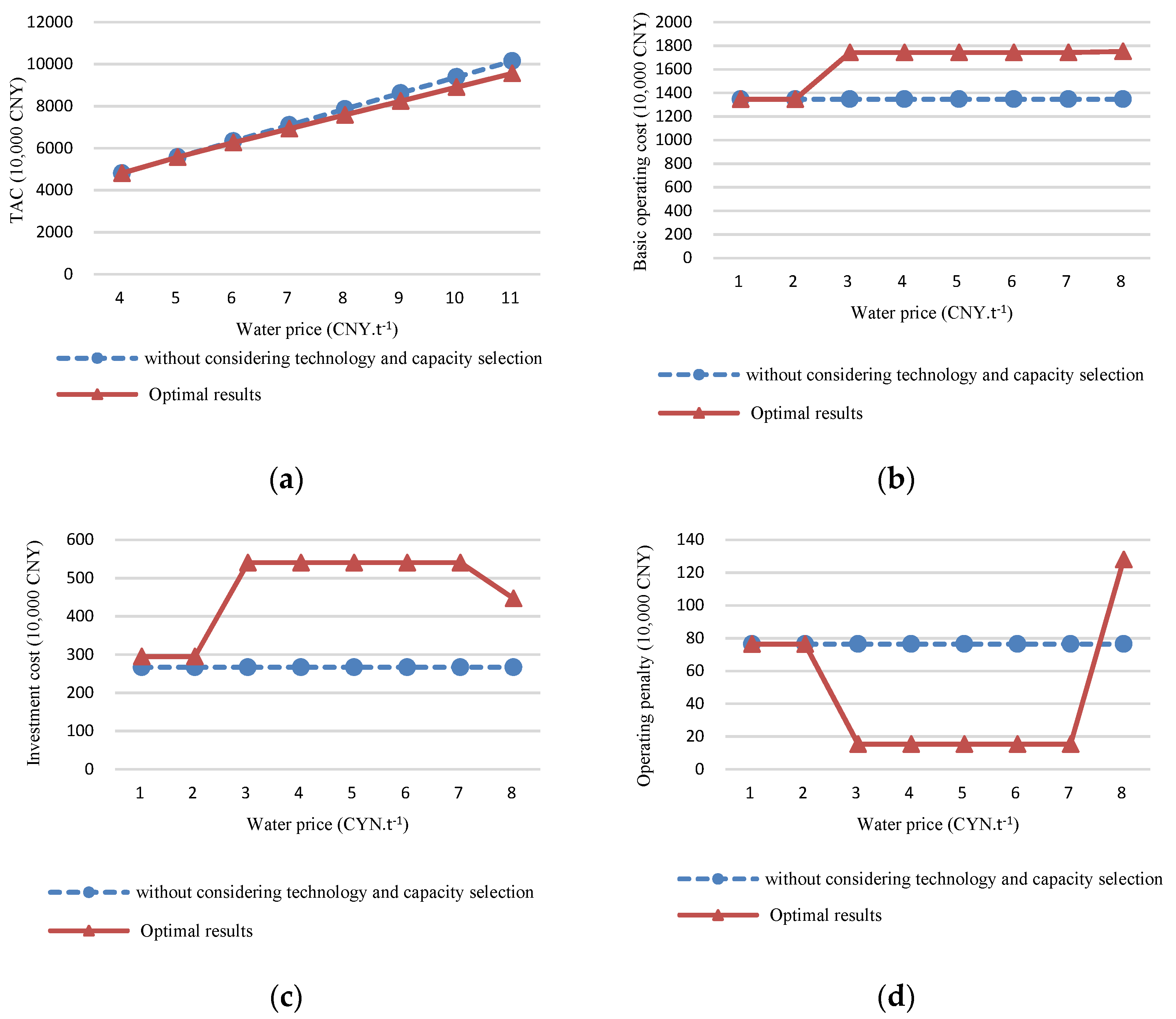
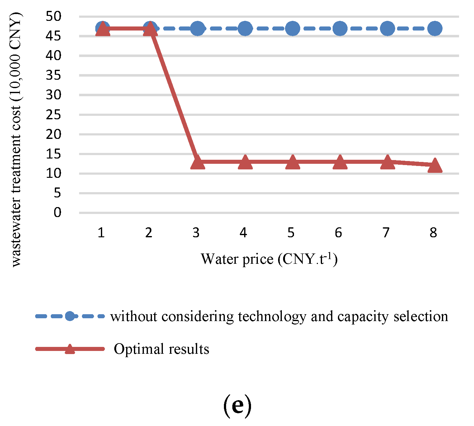
3.3. Scenario 3—Multi-Period Water Supply Network with Multiple Water Sources

In Scenario 3, the model considers multiple water resources and multi-periods in water demand simultaneously while optimizing the water supply network. The raw water cost and pre-treatment cost of surface water to produce freshwater are low. We consider surface water and municipal water as raw water resources (municipal water price is 4 CNY·t⁻¹, surface water price is 1.3 CNY·t⁻¹, and the penalty factor is 0.5). The optimal water supply network for scenario 3 is shown in Figure 6. The surface water is favorably used to produce freshwater, while the small amount of municipal water also takes part in the supply system. The desalination station takes the freshwater and produces the desalted water for seasonal demand. We use two RO units with the water capacities of 300 t·h⁻¹ and 500 t·h⁻¹ as a desalination water station.

Note that the technology and capacity selection of all scenarios are the same for the given penalty factor (i.e., 0.5). The possible reason for the same selection is that the results are optimized for a given demand, and the gap between the signal period and multi-period demand is small enough that it does not affect the technology and design capacity. It is essential to mention that the previous studies do not evaluate the technology and capacity selection by considering the penalty factor. They just select and optimize the given technology by considering the removal ratio and water production ratio. In our analysis, the technology and capacity selection are found by using the penalty factor and water price to optimize the water supply system. These results are significant for future events considering the water price for selecting and designing new water supply systems. However, the penalty factor for optimal technology and capacity selection is equally important for a single period and multi-period demand variations. The water properties of water sinks in different time periods are shown in

Table 8. Water property of water sinks after optimization (Scenario 3).

	Period	T1	T2	T3	T4
Makeup of circulating water	Conductivity (μs·cm−1)	546.74	608.25	576.79	539.13
	Turbidity (NTU)	0.48	0.14	0.31	0.52
	COD (mg·L−1)	2.29	2.47	2.38	2.27
Desalted water	Conductivity (μs·cm−1)	1.56	1.74	1.65	1.54
	Turbidity (NTU)	0.01	0.00	0.00	0.01
	COD (mg·L−1)	0.33	0.35	0.34	0.32
Wastewater	Conductivity (μs·cm−1)	1653.49	1741.50	1689.17	1638.12
	Turbidity (NTU)	22.22	32.27	28.28	21.37
	COD (mg·L−1)	35.34	50.98	44.58	33.94

. Although the water properties obtained in different seasons are slightly different, the fluctuation range is not broad, and they can meet the water property requirements of water sinks.

The costs comparison of optimization with and without considering multiple water resources, technology, and capacity selection are shown in Figure 7. The results show that by considering multiple water resources, technology, and capacity selection, the TAC is reduced by 1134.54 × 10⁴ CNY·y⁻¹. Because lower-priced surface water is used, the raw water cost is reduced by 1528.16 × 10⁴ CNY·y⁻¹, the operating cost of the desalination unit is unchanged. The operating penalty cost is reduced by 47.99 × 10⁴ CNY·y⁻¹, but the investment cost increased by 16.95 × 10⁴ CNY·y⁻¹. Moreover, because we also produce freshwater from surface water in a multi-resources scheme, RWTS needs to be used, which is why the operating and investment costs increased by 254.69 × 10⁴ CNY·y⁻¹ and 153 × 10⁴ CNY·y⁻¹, respectively. The wastewater treatment cost increased by 5.87 × 10⁴ CNY·y⁻¹.

As shown in Figure 7, the results are presented for the existing supply system for a given case study. The results show a significant economic gain for the total annual cost (TAC). The current approach is equally suitable for new water network design. In order to optimize the new industrial water supply systems, the operational status strategy along with flowrate allocation must be included in the model during the design phase of the network.

Compared with the literature, Liu et al. (2017) [28] and Ang et al. (2019) [29] consider the multi-period methodology with regeneration units, similar to the desalination station used in our study to produce desalted water. The operational status strategy for regeneration units can be integrated with the previous models in such a way that can define the objective function to minimize the total annualized cost. The operational status strategy can be considered simultaneously with the property-based flow allocation models to achieve better optimization results in the synthesis of industrial water networks. The presented approach can be considered as a part of the industrial water network for a new and/or existing network because the overall objective in our study and other literature studies is to minimize the total annualized cost.

4. Conclusions

This work proposed an MINLP model based on super-structural optimization of a multi-period water supply network, including the seasonal variation of water demand in different sinks. The different scenarios of single period and multi-period demand variations are analyzed. We analyze the effect of the variation of water price and penalty factors on the technology and capacity selection of desalination water stations. The penalty factor is the correlation between the operating status and operating costs of the desalination station at partial loads. The water supply network of a coastal oil refinery is illustrated to validate the proposed model. The results show that considering multiple water resources, technology, and capacity selection reduces the TAC by 1134.54 × 10⁴ CNY·y⁻¹ compared to the cost without considering these factors. Moreover, when the desalination units operate at partial load, and the penalty factor is significant, because of the lower operating penalty cost of multiple small capacity units, their operating cost is less than that of one large capacity unit. However, the investment cost of multiple small capacity units is higher than one large unit because of the scale effect. There is a tradeoff between the higher investment cost and the lower operating penalty cost. When municipal water price is low, it is more economical to use an RO unit for desalination. With the increasing municipal water price, it is more economical to use the IX unit for desalination. It is also established that the developed multi-period supply network model can achieve the technology and capacity selection targets for industrial desalination stations. The model is highly adaptable to existing supply systems and can be utilized to optimize new industrial water supply systems. The future work will be conducted on a large scale by including more non-conventional water resources with their pre-treatment technologies.

References

1. Gleick, P.H. Global Freshwater Resources: Soft-Path Solutions for the 21st Century. Science 2003, 302, 1524–1528. [Google Scholar] [CrossRef] [Green Version]
2. Hanjra, M.A.; Qureshi, M.E. Global Water Crisis and Future Food Security in an Era of Climate Change. Food Policy 2010, 35, 365–377. [Google Scholar] [CrossRef]
3. Gu, S.; Jenkins, A.; Gao, S.-J.; Lu, Y.; Li, H.; Li, Y.; Ferrier, R.C.; Bailey, M.; Wang, Y.; Zhang, Y. Ensuring Water Resource Security in China; the Need for Advances in Evidence-Based Policy to Support Sustainable Management. Environ. Sci. Policy 2017, 75, 65–69. [Google Scholar] [CrossRef]
4. Yuan, F.; Wei, Y.D.; Gao, J.; Chen, W. Water Crisis, Environmental Regulations and Location Dynamics of Pollution-Intensive Industries in China: A Study of the Taihu Lake Watershed. J. Clean. Prod. 2019, 216, 311–322. [Google Scholar] [CrossRef]
5. Yu, W.; Haimes, Y.Y. Multilevel Optimization for Conjunctive Use of Groundwater and Surface Water. Water Resour. Res. 1974, 10, 625–636. [Google Scholar] [CrossRef]
6. Ashwell, N.E.Q.; Peterson, J.M.; Hendricks, N.P. Optimal Groundwater Management under Climate Change and Technical Progress. Resour. Energy Econ. 2018, 51, 67–83. [Google Scholar] [CrossRef] [Green Version]
7. Watkins, D.; McKinney, D.C. Robust Optimization for Incorporating Risk and Uncertainty in Sustainable Water Resources Planning. IAHS Publ.-Ser. Proc. Rep.-Intern Assoc Hydrol. Sci. 1995, 231, 225–232. [Google Scholar]
8. Yu, L.; Xiao, Y.; Zeng, X.; Li, Y.; Fan, Y. Planning Water-Energy-Food Nexus System Management under Multi-Level and Uncertainty. J. Clean. Prod. 2020, 251, 119658. [Google Scholar] [CrossRef]
9. Fu, Z.; Zhao, H.; Wang, H.; Lu, W.; Wang, J.; Guo, H. Integrated Planning for Regional Development Planning and Water Resources Management under Uncertainty: A Case Study of Xining, China. J. Hydrol. 2017, 554, 623–634. [Google Scholar] [CrossRef]
10. Wu, X.; Zheng, Y.; Wu, B.; Tian, Y.; Han, F.; Zheng, C. Optimizing Conjunctive Use of Surface Water and Groundwater for Irrigation to Address Human-Nature Water Conflicts: A Surrogate Modeling Approach. Agric. Water Manag. 2016, 163, 380–392. [Google Scholar] [CrossRef]
11. Fazlollahi, S.; Bungener, S.L.; Mandel, P.; Becker, G.; Maréchal, F. Multi-Objectives, Multi-Period Optimization of District Energy Systems: I. Selection of Typical Operating Periods. Comput. Chem. Eng. 2014, 65, 54–66. [Google Scholar] [CrossRef] [Green Version]
12. Bungener, S.; Hackl, R.; Van Eetvelde, G.; Harvey, S.; Marechal, F. Multi-Period Analysis of Heat Integration Measures in Industrial Clusters. Energy 2015, 93, 220–234. [Google Scholar] [CrossRef]
13. Ahmad, M.I.; Zhang, N.; Jobson, M.; Chen, L. Multi-Period Design of Heat Exchanger Networks. Chem. Eng. Res. Des. 2012, 90, 1883–1895. [Google Scholar] [CrossRef]
14. Almansoori, A.; Shah, N. Design and Operation of a Future Hydrogen Supply Chain: Multi-Period Model. Int. J. Hydrogen Energy 2009, 34, 7883–7897. [Google Scholar] [CrossRef]
15. Ahmad, M.I.; Zhang, N.; Jobson, M. Modelling and Optimisation for Design of Hydrogen Networks for Multi-Period Operation. J. Clean. Prod. 2010, 18, 889–899. [Google Scholar] [CrossRef]
16. Liang, X.; Kang, L.; Liu, Y. The Flexible Design for Optimization and Debottlenecking of Multiperiod Hydrogen Networks. Ind. Eng. Chem. Res. 2016, 55, 2574–2583. [Google Scholar] [CrossRef]
17. Betancourt-Torcat, A.; Almansoori, A. Multi-Period Optimization Model for the UAE Power Sector. Energy Procedia 2015, 75, 2791–2797. [Google Scholar] [CrossRef] [Green Version]
18. Gupta, V.; Grossmann, I.E. An Efficient Multiperiod MINLP Model for Optimal Planning of Offshore Oil and Gas Field Infrastructure. Ind. Eng. Chem. Res. 2012, 51, 6823–6840. [Google Scholar] [CrossRef] [Green Version]
19. Faria, D.C.; Bagajewicz, M.J. Planning Model for the Design and/or Retrofit of Industrial Water Systems. Ind. Eng. Chem. Res. 2011, 50, 3788–3797. [Google Scholar] [CrossRef]
20. Burgara-Montero, O.; Ponce-Ortega, J.M.; Serna-González, M.; El-Halwagi, M.M. Incorporation of the Seasonal Variations in the Optimal Treatment of Industrial Effluents Discharged to Watersheds. Ind. Eng. Chem. Res. 2013, 52, 5145–5160. [Google Scholar] [CrossRef]
21. Rojas-Torres, M.G.; Nápoles-Rivera, F.; Ponce-Ortega, J.M.; Serna-González, M.; El-Halwagi, M.M. Optimal Design of Sustainable Water Systems for Cities Involving Future Projections. Comput. Chem. Eng. 2014, 69, 1–15. [Google Scholar] [CrossRef]
22. Lira-Barragán, L.F.; Ponce-Ortega, J.M.; Guillén-Gosálbez, G.; El-Halwagi, M.M. Optimal Water Management under Uncertainty for Shale Gas Production. Ind. Eng. Chem. Res. 2016, 55, 1322–1335. [Google Scholar] [CrossRef]
23. Tosarkani, B.M.; Amin, S.H. A Robust Optimization Model for Designing a Wastewater Treatment Network under Uncertainty: Multi-Objective Approach. Comput. Ind. Eng. 2020, 146, 106611. [Google Scholar] [CrossRef]
24. Boix, M.; Montastruc, L.; Pibouleau, L.; Azzaro-Pantel, C.; Domenech, S. Industrial Water Management by Multiobjective Optimization: From Individual to Collective Solution through Eco-Industrial Parks. J. Clean. Prod. 2012, 22, 85–97. [Google Scholar] [CrossRef] [Green Version]
25. Bishnu, S.K.; Linke, P.; Alnouri, S.Y.; El-Halwagi, M. Multiperiod Planning of Optimal Industrial City Direct Water Reuse Networks. Ind. Eng. Chem. Res. 2014, 53, 8844–8865. [Google Scholar] [CrossRef]
26. Arredondo-Ramírez, K.; Rubio-Castro, E.; Nápoles-Rivera, F.; Ponce-Ortega, J.M.; Serna-González, M.; El-Halwagi, M.M. Optimal Design of Agricultural Water Systems with Multiperiod Collection, Storage, and Distribution. Agric. Water Manag. 2015, 152, 161–172. [Google Scholar] [CrossRef]
27. Leong, Y.T.; Lee, J.-Y.; Chew, I.M.L. Incorporating Timesharing Scheme in Ecoindustrial Multiperiod Chilled and Cooling Water Network Design. Ind. Eng. Chem. Res. 2016, 55, 197–209. [Google Scholar] [CrossRef]
28. Liu, L.; Wang, J.; Song, H.; Du, J.; Yang, F. Multi-Period Water Network Management for Industrial Parks Considering Predictable Variations. Comput. Chem. Eng. 2017, 104, 172–184. [Google Scholar] [CrossRef]
29. Ang, M.S.; Duyag, J.; Tee, K.C.; Sy, C.L. A Multi-Period and Multi-Criterion Optimization Model Integrating Multiple Input Configurations, Reuse, and Disposal Options for a Wastewater Treatment Facility. J. Clean. Prod. 2019, 231, 1437–1449. [Google Scholar] [CrossRef]
30. Pérez-Uresti, S.I.; Ponce-Ortega, J.M.; Jiménez-Gutiérrez, A. A Multi-Objective Optimization Approach for Sustainable Water Management for Places with over-Exploited Water Resources. Comput. Chem. Eng. 2019, 121, 158–173. [Google Scholar] [CrossRef]
31. Nápoles-Rivera, F.; Ponce-Ortega, J.M.; El-Halwagi, M.M.; Jiménez-Gutiérrez, A. Global Optimization of Mass and Property Integration Networks with In-Plant Property Interceptors. Chem. Eng. Sci. 2010, 65, 4363–4377. [Google Scholar] [CrossRef]
32. El-Halwagi, M.M.; Glasgow, I.M.; Qin, X.; Eden, M.R. Property Integration: Componentless Design Techniques and Visualization Tools. AIChE J. 2004, 50, 1854–1869. [Google Scholar] [CrossRef]
Figure 1. The superstructure of multi-period water supply network.
Processes 09 02143 g001
Figure 2. Optimal water supply network (Scenario 1).
Processes 09 02143 g002
Figure 3. Annualized total cost distribution of the water supply network (Scenario 1).
Processes 09 02143 g003
Figure 4. Cost comparison of desalination unit cost before and after optimization: (a) operating penalty cost; (b) investment cost; (c) total cost of operating penalty and investment.
Processes 09 02143 g004aProcesses 09 02143 g004b
Figure 5. Cost comparison of desalination unit cost before and after optimization: (a) TAC; (b) basic operating cost; (c) investment cost; (d) operating penalty; (e) wastewater treatment cost.
Processes 09 02143 g005aProcesses 09 02143 g005b
Figure 6. Optimal water supply network (Scenario 3).
Processes 09 02143 g006
Figure 7. Comparison of costs with and without considering multiple water resources, unit technology, and capacity selection optimization (Scenario 3).
Processes 09 02143 g007