An Integrated Optimization Model for Industrial Energy System Retrofit with Process Scheduling, Heat Recovery, and Energy Supply System Synthesis

Abstract

The urgent need for CO${}_2$ reduction is calling upon the industry to contribute. However, changes within local energy supply systems including efficiency enhancement are bound to several economical and technical constraints, which results in interfering trade-offs that make it difficult to find the optimal investment option for CO${}_2$ mitigation. In this article, a new optimization model is presented that allows to optimize the design and operation of a supply and heat recovery system and production scheduling simultaneously. The model was used for retrofitting of a small brewery’s local energy system to identify decarbonization measures for eight potential future scenarios with different technical, economical and ecological boundary conditions. The results show that the proposed cost-optimized changes to the current energy system only slightly reduce carbon emissions if decarbonization is not enforced since the optimal solutions prioritize integration of photo voltaic (PV) modules that mainly substitute electricity purchase from grid, which is already assumed to be carbon free. However, enforcing decarbonization rates of 50% for the assumed future boundary conditions still results in cost savings compared to the current energy system. These systems contain heat pumps, thermal energy storages, electric boilers, and PV. Battery storages are only part of the optimal system configuration if low to moderate decarbonization rates below 50% are enforced. An analysis of marginal costs for units not considered in the optimal solutions shows that solar thermal collectors only require small decreases in collector cost to be selected by the solver.

1. Introduction

1.1. Background and Motivation

Despite the COVID-19 pandemic, which significantly squelched economic and social activities in 2020, global CO${}_2$ emissions only dropped by 6.4% [1]. The International Energy Agency World Energy Outlook [2] does not predict a further decrease, and the positive effect will be fading away until 2030 [3], which makes it impossible to meet the targets stated in the 2030 Climate & Energy Framework as part of the European Green Deal [4] without further human action. The need for decarbonization is emphasized through CO${}_2$-certificates and carbon taxes. The current trend of increasing energy costs is likely to continue, and thus incentives for industry to reduce energy consumption and switch to carbon-free energy supply will grow in the future. Considering allocated electricity and heat emissions to the different economic sectors, the industry is by far the largest emitting sector, with over 40% of global emissions [5] baring a huge potential for improvements.

In industry we can distinguish between so-called “hard-to-abate” sectors and sectors where decarbonization can succeed more easily. In the first group, one can find processes with very high temperatures, usage of fossil energy sources as crucial raw material, and process-related emissions of, e.g., iron and steel, chemicals, glass, and concrete production. The second group, where still large amounts of fossil fuels are used to provide process heat includes, among many other processes, the production of beer. The brewing process is a well-suited example for a promising batch process for decarbonization due to its comparably low temperature levels below 160 °C as stated by Eiholzer et al. [6] and Sturm et al. [7] and was thus considered as an exemplary case study in this article. In previous works on decarbonization of the brewing process Sturm et al. [8] evaluated biogas produced from a brewery’s waste for energy supply; several studies focused on the use of solar energy [6,9,10]; and Dumbliauskaite et al. [11] studied the integration of heat pump (HP)s and mechanical vapor recompression systems. Even though the low temperature requirements yield large potentials, a cost-optimal energy supply poses difficult tasks for the brewing industry, as they need to consider increasingly complex trade-offs between minimal costs for energy purchase and minimal equipment costs for storage, energy conversion, and on-site generation of renewable energy.

Mathematical optimization is a commonly used approach when complex trade-offs need to be considered. Frangopoulos [12] identified system synthesis, system design, and system operation as three crucial levels in optimizing energy systems that influence each other and thus need to be considered simultaneously to find optimal solutions [13]. This statement is true also for optimization of industrial energy systems where finding optimal trade-offs can be divided into three aspects that are interlinked. On the level of the production system there is (i) heat exchanger network synthesis (HENS) with the goal to optimize heat recovery and thus reduce energy costs and (ii) process scheduling, which optimizes the sequence in which production steps are carried out. On the supply side of the energy system there is (iii) supply system synthesis considering units such as steam generators, thermal energy storages, chillers, combined heat and power supply units, and on-site generation of renewable energy with the goal to provide the required energy demands at minimal costs.

Considering these aspects individually, either energy costs (process scheduling and HENS) or energy demand profiles (supply system synthesis and HENS) need to be prescribed. However, in cases where the design and operation of the energy supply system itself are also subject to changes, energy costs cannot be prescribed as they are the result of the aforementioned optimization. Similarly, optimization of heat recovery by means of HENS can be subject to temporal changes in the process schedule and thus both heat recovery potentials and demand profiles are not fixed. Following sequential approaches or considering only certain aspects thus leads to sub-optimal solutions for changes in the considered energy system, especially for batch processes. In this regard, Leenders et al. [14] stated that operation of the production system and of the energy supply system need to be optimized simultaneously to obtain better solutions since separated planning in general increases total costs. In the following, a review of important works on these aspects is presented with a focus on those considering trade-offs between investment and energy costs.

1.2. Literature Review on Energy System Optimization for Industrial Batch Processes

Regarding non-continuous or batch processes such as the brewing process, optimal process scheduling can include various optimization criteria such as minimizing makespan or down-times or maximizing throughput and even social criteria as proposed by Fathollahi-Fard et al. [15]. Recently, Wang et al. [16] presented a multi-objective optimization approach to improve the carbon footprint of the process and to minimize makespan. However, in breweries, production rates can be far below 100% capacity and thus optimization criteria such as minimizing makespan or maximizing production output are of low priority. However, scheduling also influences heat recovery potentials and thus energy costs as they highly depend on the temporal overlap of heat sources and sinks. A review article has been published on this subject by Fernandez et al. [17] in 2012. Authors who considered heat integration and process scheduling together are Adonyi et al. [18] who used an S-graph approach to minimize utility consumption, Zhao et al. [19] and Bozan et al. [20] who also used mixed-integer nonlinear programming (MINLP) formulations for scheduling and heat recovery, Chen and Chang [21] who applied an mixed-integer linear programming (MILP) formulation for the modeling of short-term and periodic scheduling problems with direct heat integration in batch plants, and Jung et al. [22] who used a non-linear programming formulation for optimal rescheduling and heat recovery. Lee and Reklaitis [23] also described the possibilities of heat integration offered by scheduling employing an MILP formulation and stated that significant savings in the utility cost of batch plants could be obtained. Majozi and various co-authors ([24,25]) also developed mathematical programming formulations for the optimization of heat-integrated batch chemical plants including a continuous-time framework, which resulted in in a drastic reduction in binary variables compared to the discrete-time formulation. This formulation was later extended for storage integration by Stamp and Majozi [26]. Recently, Magege and Majozi [27] presented a new MINLP formulation for the simultaneous optimization of the process design, scheduling, and heat integration of multipurpose batch plants using a stream-task-oriented scheduling formulation, which enables explicit description of the movements of the intermittently available streams. The optimization objective was to maximize annual net profit, which is a trade-off between production throughput, capital costs, and energy costs. The utility system, however, is prescribed and not subject to optimization. In an overview of current research on scheduling and planning problems Castro et al. [28] also presented a combined optimization model for HENS and process scheduling.

Energy supply system synthesis was addressed by Pipattanasomporn et al. [29] who presented a model for the optimal design of grid-connected distributed generation systems for industrial facilities considering electricity as a commodity without energy storage, whereas Paudyal et al. [30] present a generic model for optimal operation of industrial energy systems without capacity expansion planning. In the model by Atabay et al. [31] energy supply capacity expansion planning and unit commitment are included. They consider different energy conversion units and storage systems with the objective to identify the cost-optimal configuration and operation for the system with respect to given demand profiles for different commodities such as electricity, heating, and cooling. Wilkendorf [32] also introduced a flexible superstructure for utility system synthesis with minimum annual capital and operating costs considering fixed demand profiles. Similarly, the optimization model presented by Voll et al. [33] for utility system synthesis allows to include various types of energy and conversion units supporting part-load performance curves to supply given energy demand profiles. Various authors used a MILP-based approach called Method for analysis of INDustrial energy systems, which is a flexible optimization model for decision support and analyses of industrial energy systems [34,35,36,37]. Industrial energy systems are modeled using nodes and units that either require, store, or provide different commodities such as steam, electrical energy, or water. Both energy supply units and individual process steps can be optimized using a user-defined superstructure of alternative options. Optimization of heat recovery can be considered implicitly defining different levels of heat integration for certain processes. Optimization methods for energy supply systems have also been used in the context of domains other than industry such as micro-grids [38,39,40,41] and residential buildings [42,43,44,45].

Leenders et al. [14] addressed the interlink between the operation of the energy supply system and the production system applying a Stackelberg game between them to optimize energy costs. Since optimization of energy supply and heat recovery measures are also interlinked, optimization approaches have been developed that consider these aspects simultaneously. For example, different combinations of Rankine cycles, steam cycles, and cooling water systems were considered together with HENS for continuous operation [46,47,48,49,50]. Elsido et al. [51] considered organic Rankine cycles and and heat recovery steam cycles but also HP and combined heat and power cycles in an MINLP superstructure also for continuous operation. Hofmann et al. [52] presented a combined MILP optimization model considering heat recovery, utility system operation, and integration of a thermal energy storage (TES) system for non-continuous processes without utility system synthesis, whereas Elsido et al. [53] introduced a multi-period MINLP model that simultaneously considers synthesis of the heat exchanger network (HEN), the utility system, and TES.

1.3. Research Gap, Study Contribution, and Outline

None of the published works consider the trade-offs between scheduling, heat integration, and the optimal operation and design of the energy supply system or utility system at the same time. However, combining these aspects in a single optimization problem potentially yields improved solutions for operation and investment decision-support compared to sequential approaches or to optimization of individual aspects. The findings in Hofmann et al. [52] emphasize improved solutions for combined optimization of heat recovery and operation of energy supply units compared to sequential optimization stating less heat recovery but better supply unit efficiencies and lower primary energy consumption compared to the sequential approach.

The main contribution of the present work is a novel optimization model for cost-efficient decarbonization of a small-scale brewery, which for the first time comprises the combination of process scheduling, HENS and supply system synthesis. This reduces the risks of sub-optimal parameter selection at the interface of the individual sub-problems and thus yields potentially improved retrofit solutions for industrial energy systems. The model builds on the authors’ previous works (Halmschlager et al. [54] and Hofmann et al. [52]) and allows to simultaneously optimize various important aspects for the energy system such as time and quantity of energy purchase from the grid, the amount of on-site renewable energy production, the process schedule, heat recovery, and the selection of energy storage and conversion units. This is realized through a novel extension for stage-wise superstructure models for HENS that allows to couple the model with a scheduling formulation. Seasonal changes in production rates, energy prices, and potentials for on-site generation of renewable energy pose a challenge for model complexity. This issue is addressed using representative days for each month and an inter-day storage model to account for storage charging and discharging for prolonged periods. The model and its capabilities to optimize various aspects of industrial energy systems in non-continuous processes are demonstrated by means of a decarbonization study for a small-scale brewing process. Different future scenarios for energy prices and equipment costs were defined and optimized using the proposed model identifying cost-efficient measures for a CO${}_2$ reduction of more than 50%. Marginal costs analysis was conducted to identify the price gap for new units to be included in the optimal solution.

The remainder of the work is structured as follows. The optimization model with its sub-models and model interfaces is described in Section 2. Section 3 introduces the considered brewing process, assumptions for abstraction of the case, and the scenarios considered as boundary conditions for decarbonization. The results for the case study are presented in Section 4 and finally Section 5 concludes the article.

2. Optimization Model

The model proposed in this work is a mathematical programming formulation of the MILP class, meaning that the model constraints can only contain linear dependencies, and the variable values can be continuous or integers. The basic structure of the optimization model is shown in Figure 1 including the interfaces between the individual sub-models, which are described in more detail in this section:

• Process scheduling: The formulation presented in this work belongs to the class of time-point scheduling approaches using a predefined number of time points. The formulation employs the concept of virtual buckets, which are used to define process dependencies and to model both stream activity for the HENS and power demands for the supply system synthesis sub-models.
• HENS: The model for heat recovery is based on a modified version of Yee and Grossman’s stage-wise superstructure MINLP formulation [55]. In previous works, the authors proposed a linearized version (Beck and Hofmann [56]) and an extension for multi-period retrofit cases (Halmschlager et al. [54]), which are also used here. In the present work, a novel interface for process scheduling is introduced that allows to determine stream activity through the scheduling formulation.
• Supply system synthesis: The sub-model for structural optimization of the energy supply system is based on a unit commitment formulation for a predefined temporal horizon and includes a superstructure of suitable local energy generation units, conversion units, and storages. The units in the supply system need to satisfy power demands resulting from process scheduling and residual heating and cooling requirements from the HENS sub-model considering energy price variations, changing ambient conditions, and variations in solar irradiation, which are important for local renewable energy generation from PV and solar thermal (ST). Each unit consists of ports (e.g., thermal loads and electricity) and internal constraints defining the unit characteristics. A power-based approach similar to those by Morales-España [57] or Halmschlager et al. [54] was used. For seasonal and inter-day storage, a slightly modified version of the storage model proposed by Kotzur et al. [58] was implemented.

2.1. Objective Function

The objective for the optimization model was the minimization of total annual costs (TAC) in the overall energy system ${\mathit{TAC}}^{\mathit{total}}$, which consist of annualized costs in the supply system synthesis model ${\mathit{TAC}}^{\mathit{SSS}}$ and annualized costs in the HENS model ${\mathit{TAC}}^{\mathit{HENS}}$. It can be written as

$$\min {\mathit{TAC}}^{\mathit{total}}={\mathit{TAC}}^{\mathit{SSS}}+{\mathit{TAC}}^{\mathit{HENS}}.$$

(1)

The TAC for the supply system ${\mathit{TAC}}^{\mathit{SSS}}$ consist of annualized investment costs for all new units defined through the set ${\mathit{UNIT}}_{all}$ and depend on the unit’s nominal capacity ${\mathit{CAP}}^{\mathit{unit}}$, the capacity specific costs $c^{\mathit{unit},var}$, and step-fixed costs modeled using the binary variables $z^{\mathit{unit}}$ for unit existence and the cost-coefficient for step-fixed costs $c^{\mathit{unit},fix}$. Annualized investment costs are calculated using a predefined depreciation period $t_{dep}$. Energy costs are calculated using cost coefficients $c_t^{\mathit{power}}$ and $c^{\mathit{fuel}}$ together with the variables $P_t$ and $F_t$ for purchased energy. Index t depicts the discrete time periods.

$$\begin{array}{c}{\mathit{TAC}}^{\mathit{SSS}}=\frac{1}{t_{dep}}\sum _{unit\in {\mathit{UNIT}}_{\mathit{all}}}\left({\mathit{CAP}}^{\mathit{unit}}{c}^{\mathit{unit},var}+z^{\mathit{unit}}{c}^{\mathit{unit},fix}\right)\hfill \\ \hfill +\sum _{unit\in {\mathit{UNIT}}_{\mathit{all}}}\sum _t\left(c^{\mathit{fuel}}{F}_t+c_t^{\mathit{power}}{P}_t\right)d_t\end{array}$$

(2)

The TAC for the HENS sub-model ${\mathit{TAC}}^{\mathit{HENS}}$ consist of step-fixed costs and variable costs for new heat exchanger (HEX). Step-fixed costs are determined through binary variables $z^{type}$ with $\mathit{type}\in [Direct,UC,UIC,UH,UIH]$ depicting the existence of HEX for direct heat recovery and connection to utilities and a corresponding cost-coefficient $c^{\mathit{HEX},fix}$. Variable costs consist of discounted HEX areas ${A^{type}}^{\beta }$ where $\beta$ is the discount factor considering scaling effects and the area-specific HEX costs $c^{\mathit{HEX},var}$. Indices i and j depict the connected hot and cold streams, whereas index k determines the temperature stage the HEX is located in.

$$\begin{array}{c}{\mathit{TAC}}^{\mathit{HENS}}=\frac{c^{\mathit{HEX},fix}}{t_{dep}}\left(\sum _i\sum _j\sum _k{z}_{i,j,k}^{\mathit{Direct}}+\sum _i{z}_i^{UC}+\sum _i\sum _k{z}_{i,k}^{UIC}+\sum _j{z}_j^{UH}+\sum _j\sum _k{z}_{j,k}^{UIH}\right)\hfill \\ \hfill +\frac{c^{\mathit{HEX},var}}{t_{dep}}\left(\sum _i\sum _j\sum _k{A_{i,j,k}^{\mathit{Direct}}}^{\beta }+\sum _i{A_i^{UC}}^{\beta }+\sum _i\sum _k{A_{i,k}^{UIC}}^{\beta }+\sum _j{A_j^{UH}}^{\beta }+\sum _j\sum _k{A_{j,k}^{UIH}}^{\beta }\right)\end{array}$$

(3)

2.2. Process Scheduling Formulation

The process scheduling formulation used in this work belongs to the class of time-point scheduling approaches. In case of time-point- or time-interval-based models the time horizon is discretized by a predefined number of time points. Binary variables denote whether a certain task is performed at each time point; thus, the number of binary variables strongly depends on the number of time points. However, there is no known approach to determine the sufficient number of time points for the globally optimal solution; thus, an iterative approach is usually used, which may result in sub-optimal schedules [59]. On the contrary, these models can address general network based scheduling problems with batch sizing, due dates, material balances, and various storage policies as described by Hegyhati and Friedler [60].

The schedule of the processes $p\in \mathit{PROC}$ is defined by a binary variable that toggles process starts in each period $z_{p,t}^{PS}$. A continuous auxiliary variable $z_{p,t}^{PA}\in [0,1]$ is introduced to simplify constraints for process activity, which takes on the value 1 in the case that process p is active in a given period t. This variable yields also an interface to the HENS formulation of the overall model. If a process p has heating or cooling requirements, it is set equal to the activity variable of the corresponding heating or cooling requirements in the HENS sub-model. The link to the process start variables is established through the constraint

$$z_{p,t}^{PA}=\sum _{i=t+1-d_p}^t{z}_{p,i}^{PS}$$

(4)

which sets the process to active for the number of time intervals $d_p$ after the process start time. The constraints also ensure that only one instance of a process can be active at any time. The number of scheduled instances $n_p$ for a given period is ensured by

$$\sum _t{z}_{p,t}^{PA}=n_p.$$

(5)

Besides global limits on possible process activity, which can be set through binary constraints, temporal dependencies between the processes are modeled using constraint buckets. Each constraint bucket is defined by two helper variables $B_{b,t}^{in}\ge 0$ and $B_{b,t}^{out}\ge 0$ and represents a physical or virtual buffer between process steps. Processes can be linked to an increase or decrease in buckets either on process start or end. Using the parameters $P_{p,b,start}^{in}$, $P_{p,b,end}^{in}$, $P_{p,b,start}^{out}$, and $P_{p,b,end}^{out}$ this can be written as

$$\begin{array}{cc}\hfill B_{b,t}^{in}& =\sum _{p\in PROC}{z}_{p,t}^{PS}{P}_{p,b,start}^{in}+z_{p,t-d_p}^{PS}{P}_{p,b,end}^{in}\hfill \\ \hfill B_{b,t}^{out}& =\sum _{p\in PROC}{z}_{p,t}^{PS}{P}_{p,b,start}^{out}+z_{p,t-d_p}^{PS}{P}_{p,b,end}^{in}.\hfill \end{array}$$

(6)

The state of charge (SOC) of the constraint bucket $B_{b,t}^{SOC}$ is defined as

$$B_{b,t}^{SOC}=\sum _{i=0}^t{B}_{b,i}^{in}-B_{b,i}^{out}.$$

(7)

Thus, temporal constraints between processes can be formulated as simple constraints on the value of the constraint variables $B_{b,t}^{in}$, $B_{b,t}^{out}$, and $B_{b,t}^{SOC}$.

2.3. Heat Exchanger Network Synthesis

As mentioned above, the model for HENS is based on a linearized version (Beck and Hofmann [56]) of Yee and Grossman’s stage-wise superstructure MINLP formulation [55] with modifications for multi-period retrofit (Halmschlager et al. [54]). For detailed model descriptions, the reader is referred to these preceding publications. For a connection of the heat recovery system to scheduling formulations, the individual stream parameters (temperatures and heat capacity flow rates) can no longer be directly assigned to a time interval. Logical constraints are introduced to map certain sets of stream parameters, here called requirements, to the individual time intervals. For each item in the sets of hot streams and cold streams I and J, subsets for the individual requirements are introduced ($\mathit{IR}\left(i\right)$ and $\mathit{JR}\left(j\right)$). Another set considered in the following is the sets of heat exchange types $\mathit{TYPE}$ with the elements $\mathit{Direct}$ meaning direct HEX between two process streams, $\mathit{UH}$ and $\mathit{UC}$ meaning hot and cold utilities placed in the utility stages of the superstructure and $\mathit{UIH}$ and $\mathit{UIC}$ meaning hot and cold internal utilities that can also be placed in all other stages. New variables $z_{i,ir,t}^{\mathit{PSHr}}$ and $z_{j,jr,t}^{\mathit{PSCr}}$ were added to the model representing the activity of a certain requirement on hot and cold process streams. These variables also function as the interface to the process scheduling submodule. Additionally, binary variables $z_{i,ir,j,jr,k,t}^{\mathit{type}}$ and $z_{i,j,k,t}^{\mathit{type}}$ representing the connection between hot and cold process stream requirements and utilities are introduced.

2.3.1. Temperature Assignment

In the basic HENS model with a fixed process schedule, the inlet temperature parameters of the individual streams $T_{i,t}^{in}$ and $T_{j,t}^{in}$ are assigned directly to the corresponding temperature node variables $T_{i,1,t}^{\mathit{PSH}}$ and $T_{j,\mathit{NOK}+\mathit{1},t}^{\mathit{PSC}}$, since these temperatures are predefined:

$$T_{i,1,t}^{\mathit{PSH}}=T_{i,t}^{in}$$

(8)

$$T_{j,\mathit{NOK}+\mathit{1},t}^{\mathit{PSC}}=T_{j,t}^{in}$$

(9)

To realize an interface for the scheduling module for each stream and each time interval assignments of inlet temperatures were modeled using the binary variables depicting activity of stream requirements. The inlet temperature parameter of requirement 1 $T_{i,ir=1}^{in}$ was used as a base temperature, which is adjusted by the difference to inlet temperatures for other requirements ($ir>1$):

$$T_{i,1,t}^{\mathit{PSH}}=T_{i,ir=1}^{in}+\sum _{ir\in IR\backslash 1}(T_{i,ir}^{in}-T_{i,ir=1}^{in})z_{i,ir,t}^{\mathit{PSHr}}$$

(10)

$$T_{j,\mathit{NOK}+\mathit{1},t}^{\mathit{PSC}}=T_{j,jr=1}^{in}+\sum _{jr\in \mathit{JR}\backslash 1}(T_{j,jr}^{in}-T_{j,jr=1}^{in})z_{j,jr,t}^{\mathit{PSCr}}$$

(11)

Hot streams enter the superstructure in the first stage $k=1$, while cold streams enter in stage $k=\mathit{NOK}$, where $\mathit{NOK}$ is the number of temperature stages in the HEN superstructure.

2.3.2. Energy Balances

Since the heating and cooling requirements of the process streams are also not predefined for the individual time intervals, the energy balance equations need to be adjusted as well. The heating or cooling requirements $Q_{i,t}$ and $Q_{j,t}$ need to be fulfilled through either direct heat recovery or by utilities. In case of a soft stream the equality sign is replaced by ≤.

$$\sum _{j\in J,k\in [1,...,\mathit{NOK}]}{Q}_{i,j,k,t}^{Direct}+\sum _{u\in [\mathit{UC},\mathit{UIC}]}\sum _{uj\in J\left(u\right),k\in [1,...,\mathit{NOK}]}{Q}_{i,uj,k,t}^u=Q_{i,t},\forall i\in I,t\in [1,...,\mathit{NOT}]$$

(12)

$$\sum _{i\in I,k\in [1,...,\mathit{NOK}]}{Q}_{i,j,k,t}^{Direct}+\sum _{u\in [\mathit{UH},\mathit{UIH}]}\sum _{ui\in I\left(u\right),k\in [1,...,\mathit{NOK}]}{Q}_{ui,j,k,t}^u=Q_{j,t},\forall j\in J,t\in [1,...,\mathit{NOT}]$$

(13)

In the formulation with fixed schedule, $Q_{i,t}$ and $Q_{j,t}$ are parameters. For the scheduling interface, however, $Q_{i,t}$ and $Q_{j,t}$ are variables, and their values are determined using a big-M formulation incorporating the binary variables for requirement activity $z_{i,ir,t}^{PSHr}$ for hot streams and $z_{j,jr,t}^{PSCr}$ for cold streams. Here, $m_{i,ir}c{p}_{i,ir}$ and $m_{j,jr}c{p}_{j,jr}$ are the parameters for heat capacity flow rates for hot and cold streams.

$$Q_{i,t}=\sum _{ir\in IR}(T_{i,ir}^{in}-T_{i,ir}^{out})m_{i,ir}c{p}_{i,ir}{z}_{i,ir,t}^{PSHr},\forall i\in I,t\in [1,...,\mathit{NOT}]$$

(14)

$$Q_{j,t}=\sum _{jr\in JR}(T_{j,jr}^{out}-T_{j,jr}^{in})m_{j,jr}c{p}_{j,jr}{z}_{j,jr,t}^{PSCr},\forall j\in J,t\in [1,...,\mathit{NOT}]$$

(15)

The stage-wise energy balances are modeled similarly. Here the auxiliary variable $Q^{PSHr,aux}$ is used to incorporate the big-M formulation required for the hot stream energy balance. Depending on the temperature stage, the sum of all cooling requirements $Q_{i,ir,k,t}^{PSHr,aux}$ (only one active) needs to be fulfilled by direct heat recovery or utilities for each hot stream.

$$\begin{array}{c}\hfill \sum _{j\in Jifk\in {[1,...,\mathit{NOK}]}_{Direct}}{Q}_{i,j,k,t}^{Direct}+\sum _{u\in [\mathit{UC},\mathit{UIC}]}\sum _{uj\in J\left(u\right)ifk\in {[1,...,\mathit{NOK}]}_u}{Q}_{i,uj,k,t}^u=\sum _{ir\in IR}{Q}_{i,ir,k,t}^{PSHr,aux},\\ \hfill \forall i\in I,t\in [1,...,\mathit{NOT}],k\in [1,...,\mathit{NOK}]\end{array}$$

(16)

With the following constraints $Q_{i,ir,k,t}^{PSHr,aux}$ becomes equal to $m_{i,ir}c{p}_{i,ir}(T_{i,k,t}-T_{i,k+1,t})$ if the requirement $ir$ is active ($z_{i,ir,t}^{\mathit{PSHr}}=1$), whereas if the requirement is inactive ($z_{i,ir,t}^{\mathit{PSHr}}=0$) $Q_{i,ir,k,t}^{PSHr,aux}$ becomes equal to 0:

$$m_{i,ir}c{p}_{i,ir}((T_{i,k,t}-T_{i,k+1,t})-d{T}_{max,i}(1-z_{i,ir,t}^{PSHr}))\le Q_{i,ir,k,t}^{PSHr,aux}$$

(17)

$$m_{i,ir}c{p}_{i,ir}(T_{i,k,t}-T_{i,k+1,t})\ge Q_{i,ir,k,t}^{PSHr,aux}$$

(18)

$$d{T}_{max,i}{z}_{i,ir,t}^{PSHr}{m}_{i,ir}c{p}_{i,ir}\ge Q_{i,ir,k,t}^{PSHr,aux}$$

(19)

with

$$d{T}_{max,i}=(T_{i,ir}^{in}-T_{i,ir}^{out})$$

(20)

as big-M coefficient. Corresponding constraints are also used for stage-wise energy balances on cold streams.

$$\begin{array}{c}\hfill \sum _{i\in Iifk\in {[1,...,\mathit{NOK}]}_{Direct}}{Q}_{i,j,k,t}^{Direct}+\sum _{u\in [UH,UIH]}\sum _{ui\in I\left(u\right)ifk\in {[1,...,\mathit{NOK}]}_u}{Q}_{ui,j,k,t}^u=\sum _{jr\in jR}{Q}_{j,jr,k,t}^{PSCr,aux},\\ \hfill \forall j\in J,t\in [1,...,\mathit{NOT}],k\in [1,...,\mathit{NOK}]\end{array}$$

(21)

$$m_{j,jr}c{p}_{j,jr}((T_{j,k,t}-T_{j,k+1,t})-d{T}_{max,j}(1-z_{j,jr,t}^{PSCr}))\le Q_{j,jr,k,t}^{PSCr,aux}$$

(22)

$$m_{j,jr}c{p}_{j,jr}(T_{j,k,t}-T_{j,k+1,t})\ge Q_{j,jr,k,t}^{PSCr,aux}$$

(23)

$$d{T}_{max,j}{z}_{j,jr,t}^{PSCr}{m}_{j,jr}c{p}_{j,jr}\ge Q_{j,jr,k,t}^{PSCr,aux}$$

(24)

$$d{T}_{max,j}=(T_{j,jr}^{out}-T_{j,jr}^{in})$$

(25)

2.3.3. Logical Constraints

The variable for transferred heat $Q^{\mathit{Direct}}$ between hot streams and cold streams is constrained using the binary variable $z^{\mathit{Direct},r}$ indicating the activity of requirement combinations.

$$Q_{i,j,k,t}^{\mathit{Direct}}\le \sum _{ir\in IR}\sum _{jr\in JR}{Q}_{i,ir,j,jr,u}^{max}{z}_{i,ir,j,jr,k,t}^{Direct,r}$$

(26)

This means that direct heat recovery is only possible if one requirement combination $z_{i,ir,j,jr,k,t}^{Direct,r}$ is active. The activity of the stream connection between hot streams and cold streams i and j is enforced by the following constraint if at least one requirement combination of this stream combination is active. This means that as soon as a requirement combination is active, the overall stream combination also needs to be active.

$$z_{i,j,k,t}^{\mathit{Direct}}\ge \sum _{ir\in IR}\sum _{jr\in JR}{z}_{i,ir,j,jr,k,t}^{\mathit{Direct},r}$$

(27)

The requirement activities on a stream yield an upper bound for all requirement connections from this stream to any another. Thus, if a requirement $ir$ or $jr$ is not active in time interval t, no requirement combination with any other stream is possible.

$$z_{i,ir,j,jr,k,t}^{type,r}\le z_{i,ir,t}^{\mathit{PSHr}},\forall type\in [\mathit{Direct},\mathit{UC},\mathit{UIC}]$$

(28)

$$z_{i,ir,j,jr,k,t}^{type,r}\le z_{j,jr,t}^{\mathit{PSCr}},\forall type\in [\mathit{Direct},\mathit{UH},\mathit{UIH}]$$

(29)

For any stream only one requirement can be active at a time. This, however, is enforced in the process scheduling sub-model.

2.4. Example Case for Scheduling-HENS Interface

In order to demonstrate the interface between the process scheduling formulation and the HENS model, a very simple scheduling problem is considered. Two identical batches including three process steps need to be scheduled so that no pauses between process steps occur within one batch and that only one instance of each process is scheduled at any time interval. The process steps are summarized in

Table 1. Process requirements for example case.

Process Nr.	T${}^{in}$	T${}^{out}$	mcp	Power Dem.	Duration
	(°C)	(°C)	(MW/K)	(MW)	(h)
1	20	100	10	20	1
2	–	–	–	20	3
3	100	5	10	20	1

. All process steps have a power demand of 20 MW and an additional power demand through supply of electrical heating and cooling. For heating an efficiency of 0.95 and for cooling a coefficient of performance of 2 was assumed.

The objective for this example problem was to minimize energy costs and thus investment costs were neglected. The order of the process steps is enforced through individual buckets that the processes add to or consume from. Process 1 adds one unit to the constraint bucket 1 at process end; process 2 consumes one unit from bucket 1 at process start and adds one unit to bucket 2 at process end; and finally process 3 consumes one unit from bucket 2 at process start. The no-pause constraint is realized by enforcing the state-of-charge of the virtual buckets (Equation (7)) to be zero at all times. Figure 2 shows the optimal schedules and the realized electricity costs. If heat recovery was allowed with a minimum approach temperature of 5 °C in the HEX, the energy costs for this period were €22,150, whereas when heat recovery was prohibited, costs were €37,963. Since for process steps 1 and 3 electricity demand is very high without heat recovery, the optimal solution is to schedule these steps in low-price periods.

2.5. Supply System Synthesis

The energy supply system includes energy nodes for power, heating and cooling at different temperature levels. Every node is defined as an energy balance for every time period. Energy flows into the nodes can either come from conversion units, from storages, from local renewable generation, from a grid-connection or from the production process (e.g., excess heat from the HENS sub-model). Similarly, energy flows from the nodes can go to conversion units (e.g., HPs or electric boiler (EB)s), to storages, to the grid or to the process to fulfill a demand. Demands can come either from the HENS sub-model as residual heating or cooling requirements after heat recovery or from the process scheduling sub-model as power, heating or cooling requirements. The utility levels (HENS), buckets and processes (process scheduling) connected to energy node x are summarized in the set $L\left(x\right)$. Heating $Q_{ui,j,k,t}^u$ or cooling $Q_{ui,j,k,t}^u$ demands from the HENS sub-model come from the utility levels associated with node x and are expressed as

$$E_{x,t}^{\mathit{dem},\mathit{HENS}}=\sum _{u\in L\left(x\right)}\sum _{ui\in I\left(u\right),k\in [1,...,\mathit{NOK}]}{Q}_{ui,j,k,t}^u-\sum _{u\in L\left(x\right)}\sum _{uj\in J\left(u\right),k\in [1,...,\mathit{NOK}]}{Q}_{i,uj,k,t}^u,$$

(30)

whereas demands coming from the scheduling sub-model are defined using the variables for process activity $z_{p,t}^{\mathit{PA}}$ and specific energy consumption $e_p^{\mathit{dem}}$ or through the variables depicting changes in the constraint buckets $B_{b,t}^{in}$ and $B_{b,t}^{out}$.

$$E_{x,t}^{\mathit{dem},\mathit{scheduling}}=\sum _{p\in L\left(x\right)}{z}_{p,t}^{\mathit{PA}}{e}_p^{\mathit{dem}}+\sum _{b\in L\left(x\right)}{B}_{b,t}^{out}-\sum _b{B}_{b,t}^{in}$$

(31)

In the simplified unit models used in this work, variables for capacities ${\mathit{CAP}}^{\mathit{unit}}$ represent the design specification that defines the unit’s costs. For example, for a steam boiler, the capacity is its maximum thermal output, whereas for a thermal or electrical storage unit, the capacity corresponds to its maximum stored energy. For PV or ST panels, the capacity corresponds to the the units module area. Minimum and maximum available unit capacities (${\mathit{CAP}}_{\mathit{min}}^{\mathit{unit}}$ and ${\mathit{CAP}}_{\mathit{max}}^{\mathit{unit}}$) can be specified, which are enforced using binary variables $z^{\mathit{SSS},\mathit{unit}}$.

$${\mathit{CAP}}_{\mathit{min}}^{\mathit{unit}}{z}^{\mathit{unit}}\le {\mathit{CAP}}^{\mathit{unit}}\le {\mathit{CAP}}_{\mathit{max}}^{\mathit{unit}}{z}^{\mathit{unit}},\forall \mathit{unit}\in \mathit{UNIT}$$

(32)

2.5.1. Conversion Units

Conversion units are units that receive one form of energy as input and transform it into another. A gas boiler (GB), for instance, uses either natural gas or biogas and turns it into steam or hot water. Similarly, HPs use excess heat and electrical power and convert it into useful heat. These units are modeled using predefined temperature levels for heat production units and linear efficiencies. Minimum part load constraints were not considered in this work in order to reduce computational complexity.

The energy consumption $E_{in,t}^{\mathit{unit}}$ for a GB and an EB is then related to its output $E_{out,t}^{\mathit{unit}}$ and its nominal capacity ${\mathit{CAP}}^{\mathit{unit}}$ using efficiency coefficients $f_0^{\mathit{unit}}$ and $f_1^{\mathit{unit}}$.

$$\begin{array}{c}{E}_{in,t}^{\mathit{unit}}=f_0^{\mathit{unit}}{\mathit{CAP}}^{\mathit{unit}}+f_1^{\mathit{unit}}{E}_{out,t}^{\mathit{unit}},\hfill \\ \hfill \forall \mathit{unit}\in \{{\mathit{UNIT}}_{\mathit{EB}},{\mathit{UNIT}}_{\mathit{GB}}\}\forall t\in [1,...,\mathit{NOT}]\end{array}$$

(33)

In the case of constant efficiencies ${\eta }^{\mathit{unit}}$ the equation can be simplified to

$$E_{in,t}^{\mathit{unit}}{\eta }^{\mathit{unit}}=E_{out,t}^{\mathit{unit}},\forall \mathit{unit}\in \{{\mathit{UNIT}}_{\mathit{EB}},{\mathit{UNIT}}_{\mathit{GB}}\}\forall t\in [1,...,\mathit{NOT}].$$

(34)

For HPs, the efficiency is expressed as the coefficient of performance ${\mathit{COP}}^{\mathit{HP}}$, which is a function of utilization temperature $T_U$, source temperature $T_{source}$, and the second law efficiency ${\eta }_{\mathit{Carnot}}^{\mathit{HP}}$.

$$\begin{array}{cc}\hfill {\mathit{COP}}^{\mathit{HP}}& ={\eta }_{\mathit{Carnot}}^{\mathit{HP}}\frac{T_U}{T_U-T_{\mathit{source}}}\hfill \end{array}$$

(35)

For HPs the correlations between heat input $Q_{in,t}^{\mathit{unit}}$, heat output $Q_{out,t}^{\mathit{unit}}$, and power $P_t^{\mathit{unit}}$ are

$$P_t^{\mathit{unit}}=\frac{Q_{out,t}^{\mathit{unit}}}{{\mathit{COP}}^{\mathit{unit}}},\forall \mathit{unit}\in {\mathit{UNIT}}_{\mathit{HP}}\forall t\in [1,...,\mathit{NOT}]$$

(36)

and

$$P_t^{\mathit{unit}}+Q_{in,t}^{\mathit{unit}}=Q_{out,t}^{\mathit{unit}},\forall \mathit{unit}\in {\mathit{UNIT}}_{\mathit{HP}}\forall t\in [1,...,\mathit{NOT}].$$

(37)

2.5.2. On-Site Renewable Energy Generation

The efficiency of ST modules ${\eta }_{ST}^{unit}$ is modeled by

$${\eta }_{ST}^{unit}={\eta }_0-a_1\frac{T_m-T_a}{I_t}-a_2\frac{{(T_m-T_a)}^2}{I_t}$$

(38)

and depends on the mean temperature between flow- and return-side temperature of the collector $T_m$, the ambient air temperature $T_a$, and the solar irradiation $I_t$. The parameters ${\eta }_0$, $a_1$, and $a_2$ depend on the collector type and are available for all tested collectors according to ASHRAE standards [61] as well as for collectors tested according to European Standards [62]. The heat output of ST modules $E_{out,t}^{\mathit{ST}}$ is modeled by

$$E_{out,t}^{\mathit{unit}}\le {\mathit{I}}_t{\eta }_t{\mathit{CAP}}^{\mathit{unit}},\forall \mathit{unit}\in {\mathit{UNIT}}_{\mathit{ST}}\forall t\in [1,...,\mathit{NOT}].$$

(39)

The yield of PV modules is also modeled using Equation (39) with constant efficiency ${\eta }_{PV}$.

2.5.3. Storage Units

The current SOC ${\mathit{SOC}}_t^{\mathit{unit}}$ is used for modeling storage units. Two variables (${\mathit{E}}_{in,t}^{\mathit{unit}}$ and ${\mathit{E}}_{out,t}^{\mathit{unit}}$) are used to describe charging and discharging. The losses during charging and discharging processes are considered using the corresponding efficiencies ${\eta }^{\mathit{unit},\mathit{c}}$ and ${\eta }^{\mathit{unit},\mathit{d}}$. Energy balance equations are connecting SOC, charging, and discharging. Here, $d_t$ is the interval duration.

$$\begin{array}{c}{\mathit{SOC}}_{t+1}^{\mathit{unit}}-{\mathit{SOC}}_t^{\mathit{unit}}=d_t({\eta }^{\mathit{unit},\mathit{c}}{\mathit{E}}_{in,t}^{\mathit{unit}}-\frac{1}{{\eta }^{\mathit{unit},\mathit{d}}}{\mathit{E}}_{out,t}^{\mathit{unit}})\\ \forall \mathit{unit}\in {\mathit{UNIT}}_{\mathit{S}}\forall t\in [1,...,\mathit{NOT}].\end{array}$$

(40)

Since inter-day and seasonal storage was considered in this work, the storage formulation presented by Kotzur et al. [58], which was also applied by van der Hejde et al. [63], was used and slightly modified. In this model, cyclic energy storage is not enforced for each representative day but only for the entire optimization period, which in this case is one year. In contrast to the model used by Kotzur et al., the SOC profiles for each day s are connected in a way, such that $SO{C}_{s+1,t=0}\le SO{C}_{s,t=NOT}$. This means that the storage is allowed to discharge energy at the boundary of consecutive days (Figure 3). This allows for additional flexibility, which is important for efficient use of on-site production of renewable energy and accumulation of excess heat for later usage for non-cyclic production schedules. The formulation can account for curtailment of local renewables production and reduced excess heat usage between different days modeled using the same representative days. Thus, this influences storage sizing in a positive way but does not jeopardize the operability of the system.

Since the model used in this work is very similar to the model proposed by Kotzur et al. [58], model equations are only briefly stated in Appendix A.1 without detailed description.

3. Brewery Case Study

To show the features and functionality of the proposed method, it was applied to the case study of a small-scale brewery. The back-laying motivation for choosing the brewing process as a case study was addressed in the introduction. Thus, in this Section required inputs for the individual optimization tasks and necessary additional evaluations, such as representative period selection, are derived from the information about the case study and presented here.

The brewing process studied in this work is characterized through its various degrees of freedom when it comes to changes in the energy system. Beer is brewed in batches, which allows scheduling of single production steps. In this use case, which is related to a small brewery production process, production does not exceed one batch per day, and the monthly number of brewing days varies throughout the year. In general, brewing converts the input streams malt, brewing water, hops, and yeast to the final product beer and side products grains and separated turbidities. The main process steps and auxiliary process steps are summarized in the Appendix A.3 in

Table A3. Main (upper part of table) and auxiliary (lower part of table) process steps of brewing.

Process Step	Process Description
Milling	Malt grains are crushed by the use of electrical energy.
Mashing	Malt and warm brewing water from the brewing water tank are mixed and heated up in a defined process to dissolve nutrients from the malt and transfer them to the brewing water. The process time lies in the range of about one hour. Heat supply is realized through steam.
Lautering	Mash and brewing water are mixed in another tank. Electric drives supply the required energy. No additional thermal energy is needed. The process takes several hours. At the end, solids (so-called grains) are separated and the resulting wort is fed to the next process step.
Wort boiling	Hops is added and the wort is brought to a boil. During this process, the volume of the wort is reduced by heating, boiling and partial evaporation (up to 10%). The total process time is several hours.
Whirlpool	In this process step the use of electrical energy ensures that turbid matter and solids are separated from the final product stream after wort boiling.
Cooling	Subsequently, the hot product stream must be cooled from approximately 100 °C to below 10 °C in a short period of time. The heat extracted from cooling is often used, also in this use-case, to heat up brewing water for subsequent brewing processes.
Fermentation	After the yeast has been added, the intermediate product is cooled for the duration of fermentation, which takes several days (approx. 4–7). During this process, sugar molecules (from the malt used in the beginning of the brewing process) are converted into alcohol and CO${}_2$. Depending on the yeast strain (top- or bottom-fermented), the fermentation temperature is determined (usually 5–18 °C).
Conditioning	After fermentation is complete, the beer is further cooled (around 0 °C for several weeks in cold rooms or refrigerated containers.
Packaging	The final step involves bottling or kegging of the finished product.
Cleaning in Place	The tanks (mashing and wort boiling tank, lautering tank + whirlpool) are cleaned by rinsing with cleaning water, basic and acidic solutions. The basic solution is provided at around 80 °C.
Cleaning of packaging	Usually bottle and keg washers are installed using hot water to clean the packaging containers.
Supply of cooling	To remove excess heat from the fermentation and conditioning process usually compression chillers together with an appropriate working fluid are used. These units consume electric power in the compressor, provide cooling on a low temperature level and release excess heat on a higher level.
Space heating and cooling	Space heating and cooling needs to be provided for work spaces in the production area and offices. For space heating usually hot water, usually provided by excess heat from steam generation units, is used. For space cooling electricity for air conditioning is required.
Information technology and lighting	Electricity is required to cover the demand for lighting of offices and production areas. Furthermore, IT infrastructure is another consumer of electric power.

. For the optimization model this leads to a production process having hot and cold streams with potentials for heat recovery and heat supply at intermediate temperature levels. The latter implies that a low-grade heat supply could be an option. The process is suitable for renewable energy supply due to its low temperature requirements (below 120 °C).

In Section 3.1 the defined energy supply and production systems are explained. Furthermore, the derived stream table to depict heat and cooling load requirements is presented as well as two thermal energy requirements, which are not included in the stream table as they do not require specific heat loads but rather a required target temperature needs to be reached at a certain point during the batch process defined through the process schedule. Section 3.2 gives an overview how one production year was simplified to derive representative days for the brewery use case optimization. Finally, in Section 3.3 the defined scenarios for which a run of the optimization model analyzed in Section 4 is explained.

3.1. Energy and Production System

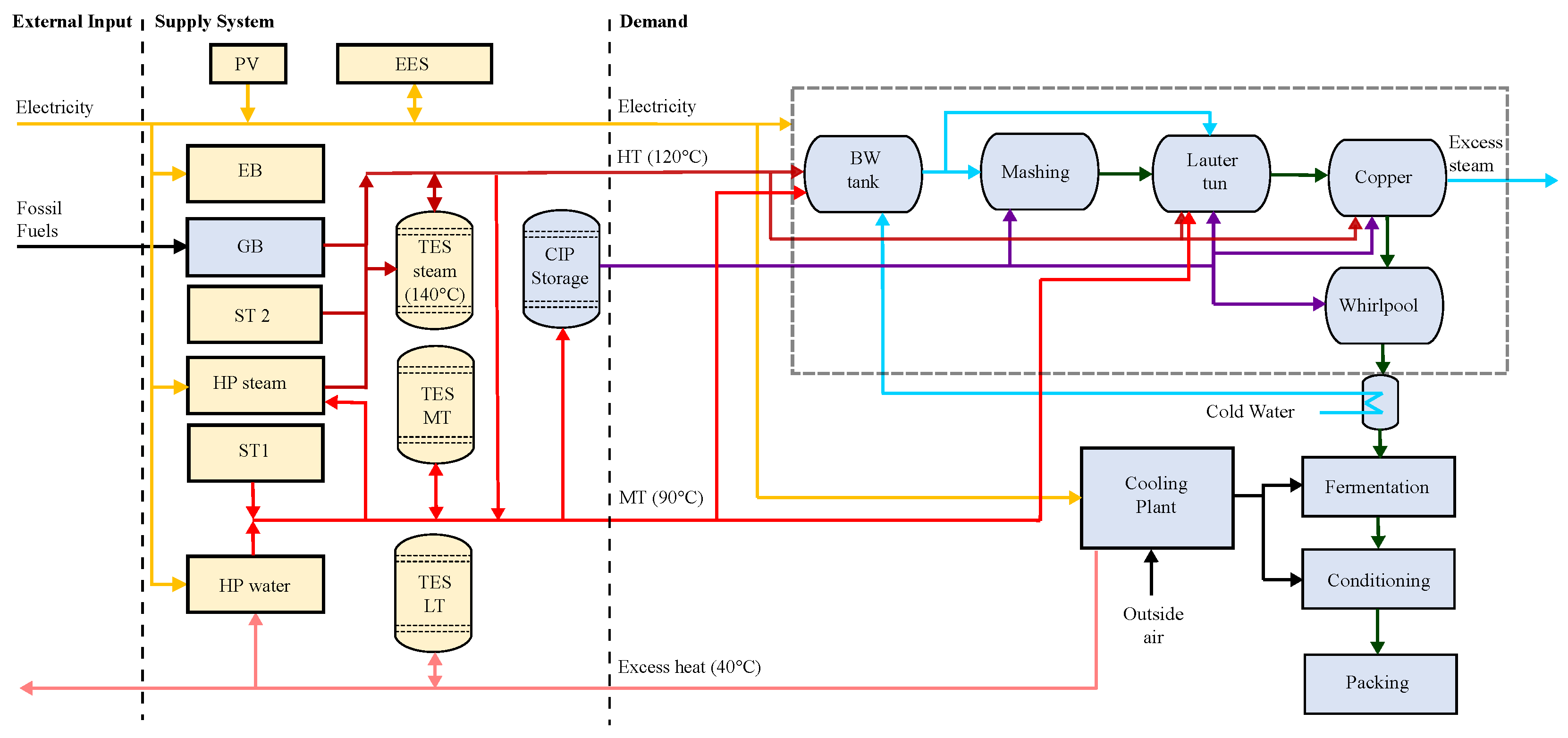
The superstructure considered for the energy supply system is shown in Figure 4. The status quo, a GB covering all heating requirements, is highlighted in grey, whereas potential additions to the supply system are highlighted in yellow. For heat supply, ST collectors (ST1 and ST2 with different temperature levels), an EB and HPs for the supply of hot water and direct steam production are considered. In addition, TES at different temperature levels (40 °C, 90 °C, and 140 °C) can be added to the system. For renewable power production, PV and an electric energy storage (EES) can be selected. Further information about the units are summarized in the Appendix A.2,

Table A1. Considered energy supply units.

Unit	Parameter	Value
Gas boiler:
GB
Efficiency	$\eta$ (–)	0.94
Steam temperature	$T_{steam}$ (°C)	120
Fixed costs	c${}^{fix}$ (€)	25,000
Variable costs	c${}^{var}$ (€/kW)	50
Electric boiler:
EB
Efficiency	$\eta$ (–)	0.98
Steam temperature	$T_{steam}$ (°C)	120
Fixed costs	c${}^{fix}$ (€)	0
Variable costs	c${}^{var}$ (€/kW)	150
Steam Heat-pump
HP steam
Efficiency	$\eta$ (–)	0.4
Source Temperature	T${}_{source}$ (°C)	80/90
Sink Temperature	T${}_{sink}$ (°C)	120/150
Temperature difference	ΔT (°C)	5
Fixed costs	c${}^{fix}$ (€)	35,000
Variable costs	c${}^{var}$ (€/kW)	600
Funding	(%)	30
Water heat-pump:
HP water
Efficiency	$\eta$ (–)	0.5
Source Temperature	T${}_{source}$ (°C)	35/40
Sink Temperature	T${}_{sink}$ (°C)	80/90
Temperature difference	ΔT (°C)	5
Fixed costs	c${}^{fix}$ (€)	5000
Variable costs	c${}^{var}$ (€/kW)	400
Funding	(%)	30
Photovoltaic module:
PV (LG Solar LG390Q1C-A6 NeON R)
Efficiency	$\eta$ (–)	21.5
Fixed costs	c${}^{fix}$ (€)	5000
Variable costs	c${}^{var}$ (€/m${}^2$)	250
Funding	(%)	60 [66]
Solar thermal collector:
ST 1 (MT-Power TVP Vakuum)
Inlet temperature	T${}_{in}$ (°C)	80
Outlet temperature	T${}_{out}$ (°C)	90
Efficiency	${\eta }_0$ (%)	75.9
Efficiency factor	a${}_1$ (W/(m2K))	0.509
Efficiency factor	a${}_2$ (W/(m2K2))	0.007
Fixed costs	c${}^{fix}$ (€)	2000
Variable costs	c${}^{var}$ (€/m${}^2$)	320
Funding	(%)	65 [67]
Solar thermal collector:
ST 2 (Ritter XL Solar)
Inlet temperature	T${}_{in}$ (°C)	110
Outlet temperature	T${}_{out}$ (°C)	130
Efficiency	${\eta }_0$ (%)	0.687
Efficiency factor	a${}_1$ (W/(m2K))	0.613
Efficiency factor	a${}_2$ (W/(m2K2))	0.003
Fixed costs	c${}^{fix}$ (€)	2000
Variable costs	c${}^{var}$ (€/m${}^2$)	283
Funding	(%)	65 [67]

, and

Table A2. Considered energy storage units.

Unit	Parameter	Value
Electrical energy storage system:
EES 1 (funded capacity) and EES 2 (not funded capacity)
Relative losses SOC	(%/h)	10.42 × 10${}^4$
Fixed costs	c${}^{fix}$ (€)	2000
Variable costs	c${}^{var}$ (€/kW)	500
Funding	(%)	30 (for 0–50 kWh)
Low temperature thermal energy Storage:
TES water 1
Inlet temperature	T${}_{in}$ (°C)	40
Outlet temperature	T${}_{out}$ (°C)	30
Relative losses SOC	(%/h)	0.083
Fixed costs	c${}^{fix}$ (€)	35,000
Variable costs	c${}^{var}$ (€/kW)	2500
Medium temperature thermal energy Storage:
TES water 2
Inlet temperature	T${}_{in}$ (°C)	90
Outlet temperature	T${}_{out}$ (°C)	70
Relative losses SOC	(%/h)	0.083
Fixed costs	c${}^{fix}$ (€)	35,000
Variable costs	c${}^{var}$ (€/kW)	2500
High temperature thermal energy storage:
TES steam
Inlet temperature	T${}_{in}$ (°C)	140
Outlet temperature	T${}_{out}$ (°C)	120
Relative losses SOC	(%/h)	0.167
Fixed costs	c${}^{fix}$ (€)	20.000
Variabel costs	c${}^{var}$ (€/kW)	100.000

. These units were pre-selected with regard to their technical feasibility. Biomass and biogas were not considered as there was no local supply available. The possibility of using brewery waste was also not included as processes to harvest biogas would, in this case, cross the economic boundaries of the small-scale brewery.

The main heating, cooling, and power demands of the production process are shown on the demand side in Figure 4 and are represented in the form of a stream table (

Table 2. Stream/requirements table for production days; all streams have a heat transfer coefficient of 2 kW/m²K.

	Req. Nr.	T${}^{\mathrm{in}}$	T${}^{\mathrm{out}}$	mcp	Power Dem.	Duration
Name		(°C)	(°C)	(kW/K)	(kW)	(h)
Brewing water heat up	1	12	80	19.6	–	1
Total mash heat up	2.1	63	64	268.5	37	1
Cooking mash cook	2.2	99	100	288.0	37	1
Lautering	3	–	–	–	37	2
Wort cooking heat up	4.1	99	100	639.1	37	1
Wort cooking	4.2	99	100	1274.1	37	1
Whirlpool	5	–	–	–	37	1
Wort cooling	6	97	8	19.0	–	1

). The order of the requirements corresponds to the required sequence of the individual process steps. Brewing water heat up (Req. nr. 1), however, can be scheduled without temporal restrictions.

Heating requirements not shown in the stream table are for cleaning-in-place (CIP) and reheating of the brewing water tank as these are energy requirements rather than heat load requirements. This means that for a certain point in time CIP media and brewing water need to have been heated up to a target temperature, but no hard time restrictions are imposed. For the CIP process, it was assumed that the basic rinsing solution is heated once from 50 °C to 80 °C for the first process on each brewing day and from 75 °C to 80 °C for each subsequent CIP operation to account for heat losses. Before mashing and lautering, 5500 L and 7000 L of brewing water need to be heated up to 68 °C, respectively. Thermal energy demand for space heating and for packaging and cleaning of bottles and kegs was neglected.

3.2. Selection of Representative Periods

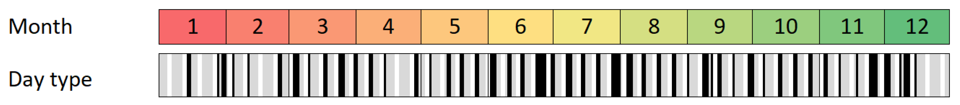
Process energy demands primarily differ between production days and days without production, whereas the electricity demand for drives, pumps, compression chillers, lightening, IT, etc. is not aligned to process activities but mainly differs between weekdays and weekends. These distinct characteristics were considered by means of three representative days for each month of the year: (i) a production day, (ii) a weekday without production, and (iii) a weekend day. This leads to a drastic reduction in computational complexity as for the process scheduling and HENS sub-models, only two distinct representative production days needed to be modeled explicitly for the entire year. For the supply system synthesis sub-model, the three representative days described above were modeled explicitly for each month, resulting in 36 explicitly modeled days. The resulting mapping is shown in Figure 5.

Average profiles for solar irradiation, ambient temperature, expected electricity costs, and power demand for the brewing process were used to derive these representative days. For ambient air temperature and irradiation data for Vienna from 2017–2019 were used [64]. The derived electricity price profiles are based on historical data of the Austrian Energy Exchange EXAA for 2019 [65]. For these parameters two sets of hourly representative profiles for each month were determined—one for weekdays (with and without brewing) and one for weekend days. Brewing days were identified by finding those n days in 2019 with the highest to $n^{th}$-highest daily electricity consumption. For the electrical base load, the actual consumption from the electrical grid for the year 2019 was used as a data base. The resulting profiles for electricity prices and electricity base demand are shown in Figure 6.

3.3. Scenarios

Based on the business-as-usual (BAU) case, changes to the existing energy system are analyzed using eight different price scenarios and boundary conditions for the time periods of 2020–2025, 2025–2030, and 2030–2035 (see

Table 3. Overview of assumptions for calculated scenarios with differences in existing units, and required decarbonization rate (DC).

Scenario	Period	Existing Unit	DC Rate (%)
Scenario 1 (BAU)	2020–2025	GB	0
Scenario 2	2020–2025	GB	0
Scenario 3	2025–2030	GB	0
Scenario 4	2030–2035	GB	0
Scenario 5	2020–2025	GB	25
Scenario 6	2020–2025	GB	50
Scenario 7	2020–2025	GB	100
Scenario 8	2020–2025	None	0

). Cost discounts due to funding of renewable technologies available on national and international levels are also considered, see, e.g., [66,67].

In the first seven scenarios the currently existing GB is still in place, while in Scenario 8 it is assumed that a replacement is required. In Scenarios 5–7 a minimum decarbonization rate is enforced, while in Scenarios 1-4 and 8 the solution is purely economic. The variations in energy-related economic boundary conditions are shown in

Table 4. Overview of development of energy and CO${}_2$ prices and investment costs for specific technologies used in the elaborated scenarios.

Parameter	2020–2025	2025–2030	2030–2035
CO${}_2$ price (€/MW) [68]	5.75	10.12	18.4
Natural gas price factor (–) [68]	1.12	1.24	1.29
Electricity amplitude factor (–)	1	1.1	1.2
Average electricity price factor (–) [68]	1.2	1.53	1.74
Cost factor EES (–)	1	0.94	0.86
Cost factor HP (–) [69]	1	0.965	0.93
Cost factor PV (–) [70]	1	0.9	0.7

. The development of the CO${}_2$ price, natural gas price, and average electricity price from 2020 to 2030 are based on a forecast by Huneke et al. from 2019 [68]. For both, natural gas and electricity, the given factors in Table 4 correspond to the increase in average values in the time period in the headline of the specific column compared to 2020 prices. In order to combine fluctuating electricity prices and the forecast for average electricity prices presented in that study, the electricity price consists of an average price, referred to as Average electricity price factor, which is aligned to the development shown in Table 4 and an hourly deviation from this average value, referred to as Electricity amplitude factor. These electricity price fluctuations are assumed to increase by 10% in the 2025–2030 scenarios and by 20% in the 2030–2035 scenarios based on the expansion of renewables. Cost factors for EES, HPs, and PV-modules that consider scale up effects and learning curves were derived from [69,70] and were used to account for a decrease in investment costs in 2025 and 2030 compared to 2020.

4. Results

The calculations and optimization were carried out on an Intel Core i7-8665U CPU with 32 GB of RAM, and CPLEX 12.9 was used as a MILP-solver. The computation time for each of the scenarios was in the range of 10 to 30 min. Investment costs are annualized with an internal depreciation period $t_{dep}$ of 10 years.

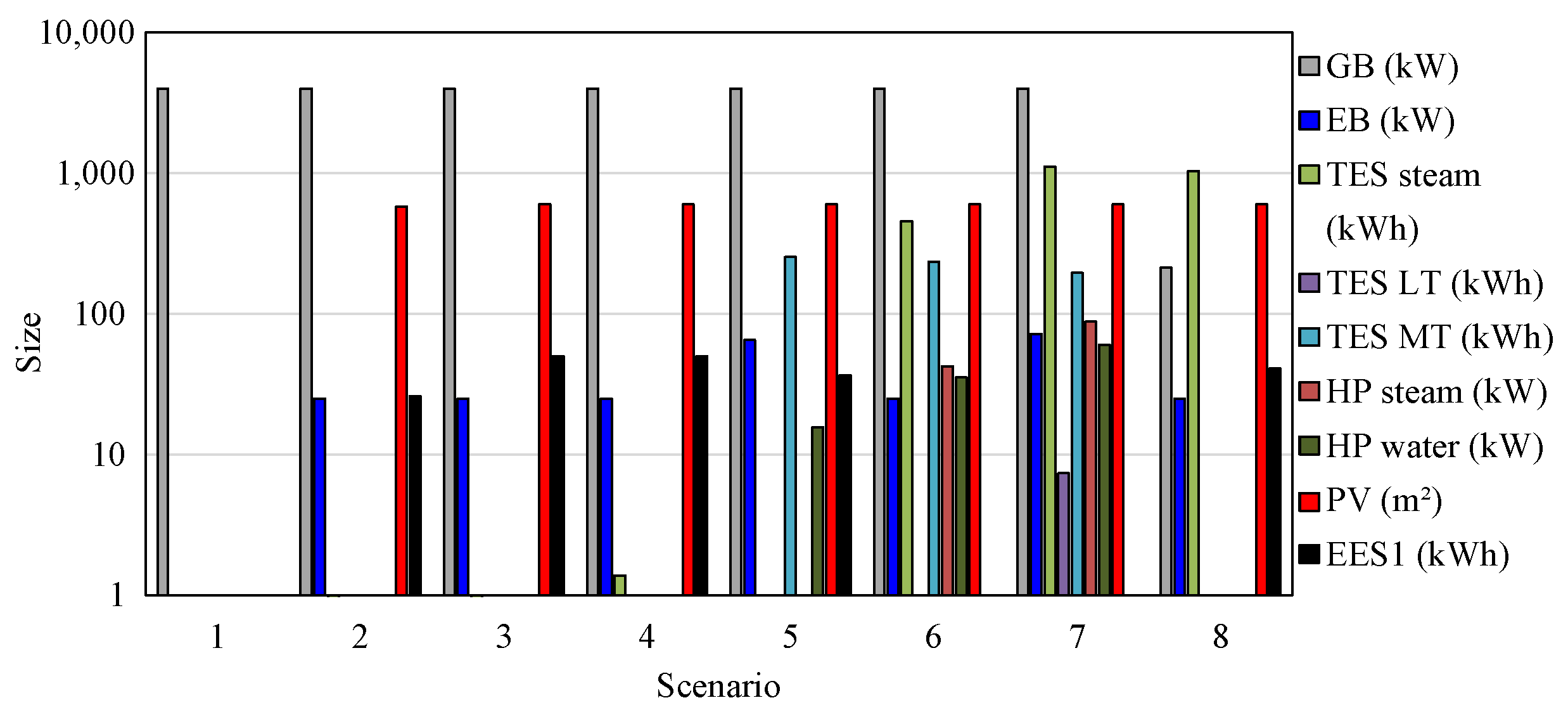
Figure 7 shows a summary of the selected unit sizes for all scenarios. Only units that are at least selected in one scenario are presented in the figure. ST was never selected and thus is not shown. The GB with a nominal power of 4 MW is part of the system in all scenarios; however, for Scenarios 1–7, the GB is preset, whereas in Scenario 8, where the existing GB has reached its end of life, it was replaced by a much smaller GB unit with 213 kW. The CIP and the brewing water tank are also not depicted as they are existing units with a fixed size.

In order to investigate how much the investment costs would have to be reduced for unused units to be part of the optimal solution, a sensitivity analysis was performed. One by one, the investment costs of the unused units were reduced to 5% of their actual investment costs, and the resulting optimal capacities were calculated. For the cases where this cost reduction resulted in the units’ introduction into the optimal system, their capacities were reduced to 50%, 25%, and 12.5% of its initial value. To calculate the maximum specific costs of a unit

$$\mathrm{\Delta }{C}^{\mathit{unit}}=C^{\mathit{unit},\mathit{base}}-\left(C^{\mathit{unit},\mathit{sens}}-0.05\frac{(c^{\mathit{unit},fix}+{\mathit{CAP}}^{\mathit{unit}}{c}^{\mathit{unit},var})}{t_{dep}}\right)$$

(41)

is defined. Here, $C^{\mathit{unit},\mathit{base}}$ refers to the resulting costs without cost reduction, while $C^{\mathit{unit},\mathit{sens}}$ are the costs with reduced investment costs. To ensure comparability, $C^{\mathit{unit},\mathit{sens}}$ is then corrected by the reduced cost values. The maximum specific costs for the respective unit to be introduced to the optimal solution can be defined as

$$C^{\mathit{unit},max}=t_{dep}\frac{\mathrm{\Delta }{C}^{\mathit{unit}}}{{\mathit{CAP}}^{\mathit{unit}}}$$

(42)

The minimum required cost reduction for economical feasibility is expressed by the difference between the actual specific costs and the maximum specific costs.

$$C^{\mathit{unit},\mathit{min}\mathit{red}}=\frac{C^{\mathit{unit},max}-C^{\mathit{unit}}}{C^{\mathit{unit}}}$$

(43)

The actual costs of the units in the optimal solutions and the required cost reduction for units that are not part of the optimal solution to be integrated are shown in Figure 8. For Scenario 7 both ST modules are close to being implemented as the threshold price is close to the actual price. The same is true for Scenario 5 where the second ST module would be implemented if the price was only around 3% lower. This analysis shows that good estimates for unit costs are necessary to really find the optimal configuration. In cases where certain technologies are not part of the optimal solution but their required cost reduction is relatively small, these alternative technologies should be included when it comes to more detailed conceptualization of decarbonization measures. Especially, for new technologies and steep learning curves this can add uncertainties to the results.

The existing and for all scenarios final HEN is shown in Figure 9. In Scenarios 5–7 heat is also supplied at 90 °C via hot water to heat up mash and to heat up brewing water. However, this heat is supplied via the same HEX also used to supply heat via steam at 120 °C.

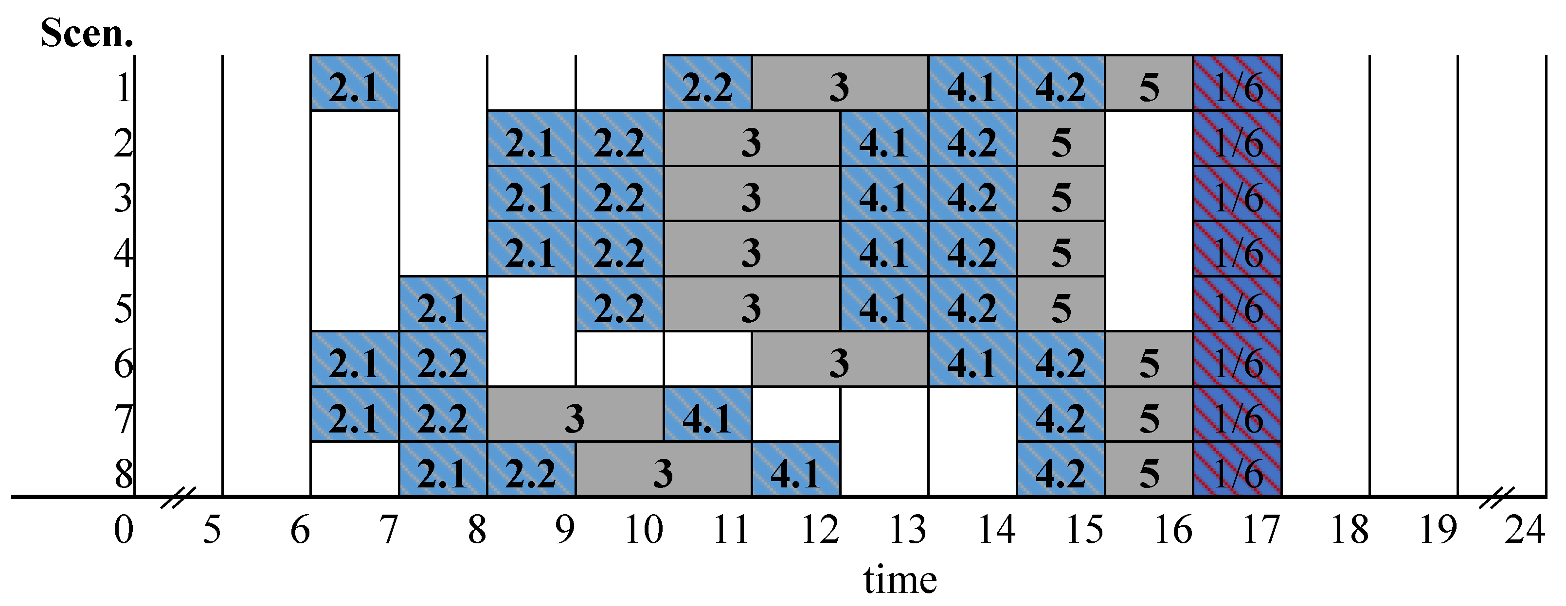
The optimized production schedule for each scenario is depicted in Figure 10. Since temperature losses over time are not considered, processes like Wort cooking heat-up and Wort cooking are not coupled to each other enabling flexibility for the scheduling. For Scenarios 2–4, which include PV, process steps requiring electricity are shifted towards times of high solar irradiation. With enforced decarbonization (Scenarios 5–7) the energy supply is increasingly electrified, and more storage capacity is added to the system, which influences the optimal schedule.

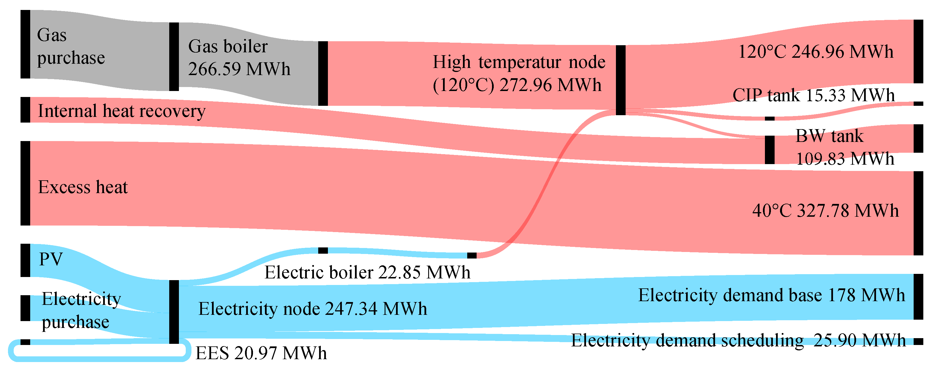
Figure 11 shows a sankey plot of the BAU scenario (Scenario 1). The high temperature heat demand of the overall brew process and the CIP system is covered by the existing GB, while the electricity needs are supplied by the electrical grid.

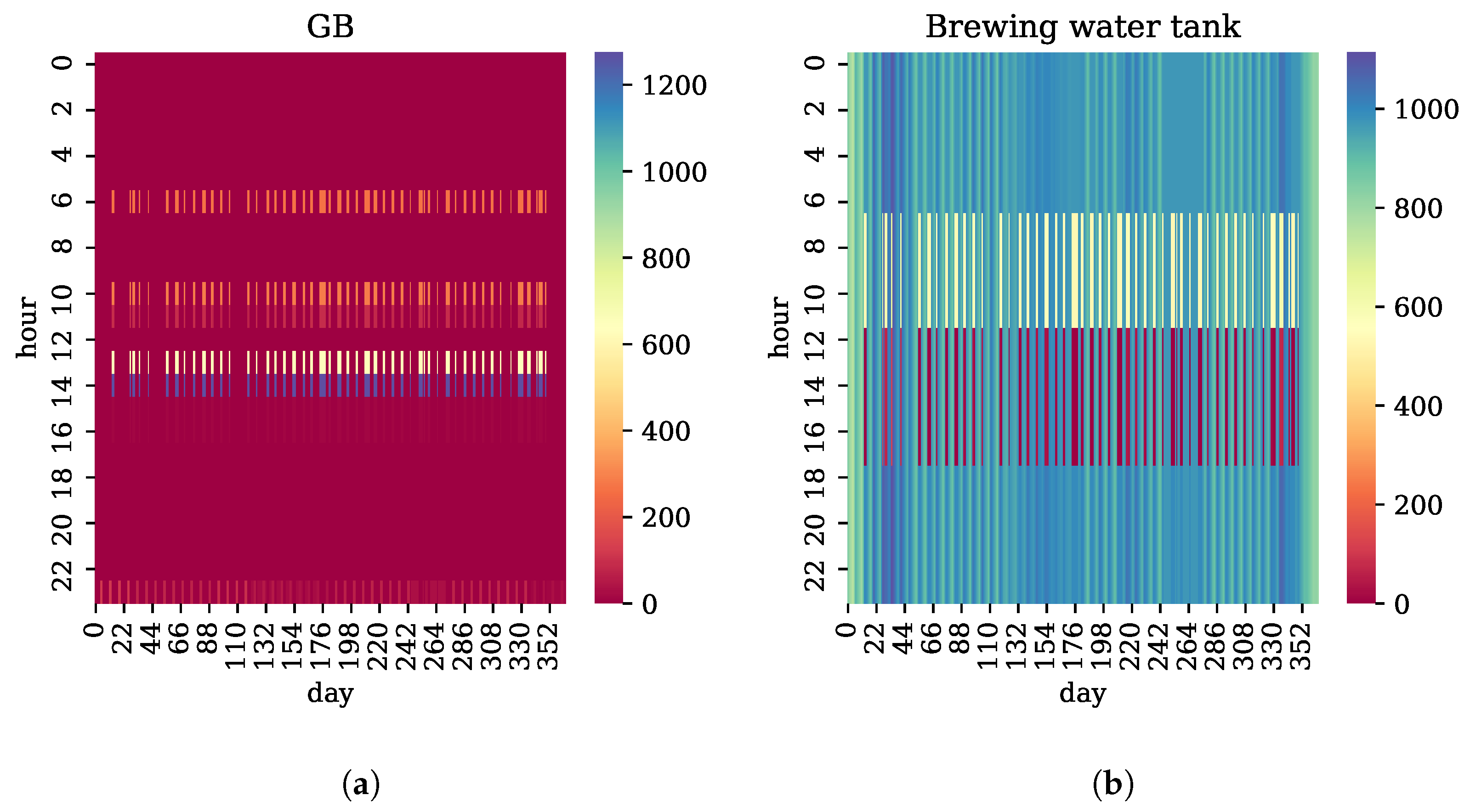
Heat loads of the GB and energy content of the brewing water tank are depicted in Figure 12 as heat maps. The GB is sufficiently large to cover all heating requirements as they occur. Interestingly, the brewing water tank is starting to discharge at 6 a.m. from approximately 70% to 50% and is further discharged at 10 a.m. to 0%. In the afternoon around 5 p.m. it is charged up for the next brew day. The overall behavior remains the same for all scenarios but for Scenario 7 (fully decarbonized) where the brewing water tank completely unloads two hours earlier at 8 a.m.

In Scenarios 2–4 the design of the energy system is similar with only differences in unit sizing. Figure 13 shows the energy flows for the optimal supply system in Scenario 2, which are very similar also in Scenarios 3 and 4. In addition to the already existing GB there is a relatively small EB with 25 kW nominal heat load (25 kW is the lower bound for the EB size); PV close to (Scenario 2) or at the capacity limit (Scenarios 3 and 4) of 600 m²; a very small steam storage of approximately 1 kWh, which is negligible; and an EES with 26 kWh capacity in Scenario 2 and 50 kWh capacity in Scenarios 3 and 4.

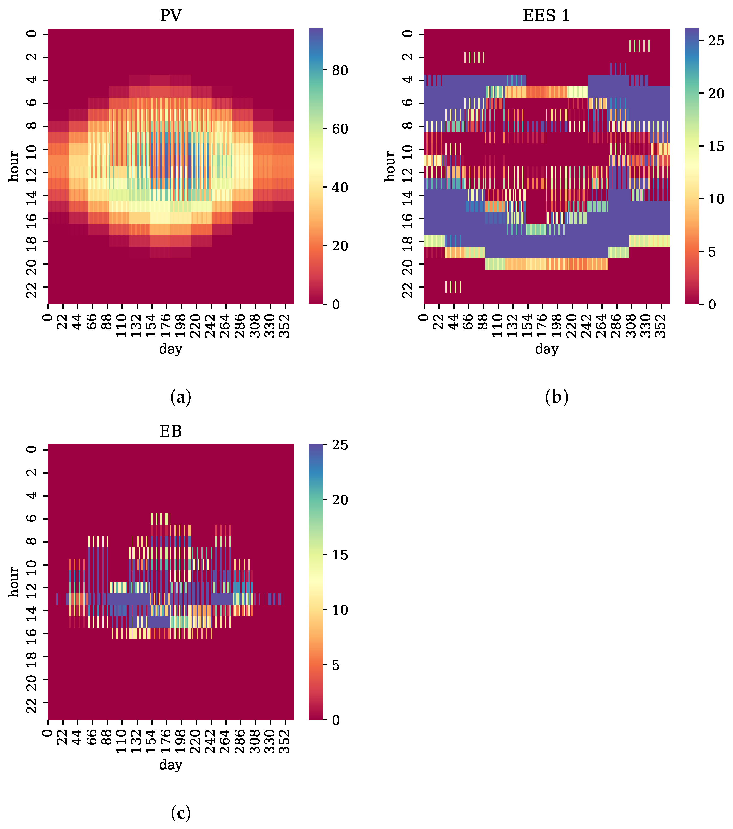
The capacity of the EES caps at 50 kWh since this was assumed to be the capacity limit for subsidies. A further increase in EES capacity would result in higher specific costs. The optimal operation and design of the EES is heavily depending on the energy prices and process scheduling as can be seen in Figure 14b where operating characteristics are shown for Scenario 2. At around 3 a.m. when electricity is cheap, the EES is charged and discharges later on the same day when electricity is needed. PV (Figure 14a) influences process scheduling as the electricity demand is shifted to the hours when PV has its highest yield. The EB (Figure 14c) is also turned on when PV production is high.

With the introduction of an enforced CO${}_2$ reduction in Scenarios 5–7, new units are introduced in the energy supply system. At a 25% reduction in Scenario 5, a water HP is included in the optimal system, while at a reduction of 50% (Scenario 6), the steam HP together with a much larger steam TES compared to Scenarios 2–4 are part of the optimal solution (Figure 7). The energy flows and the configuration of the energy supply system of the fully decarbonized brewery in Scenario 7 are shown in Figure 15. To completely substitute the GB both HP types in combination with TES on the three available temperature levels were used. The electricity purchased from the grid was increased by a factor of approximately 1.3 compared to the BAU case (Scenario 1) and by a factor of 2.6 compared to Scenario 2, where PV was already installed. Moreover, in the fully decarbonized Scenario 7 hot water at 90 °C was used to heat up the brewing water tank and the mash (see Figure 9).

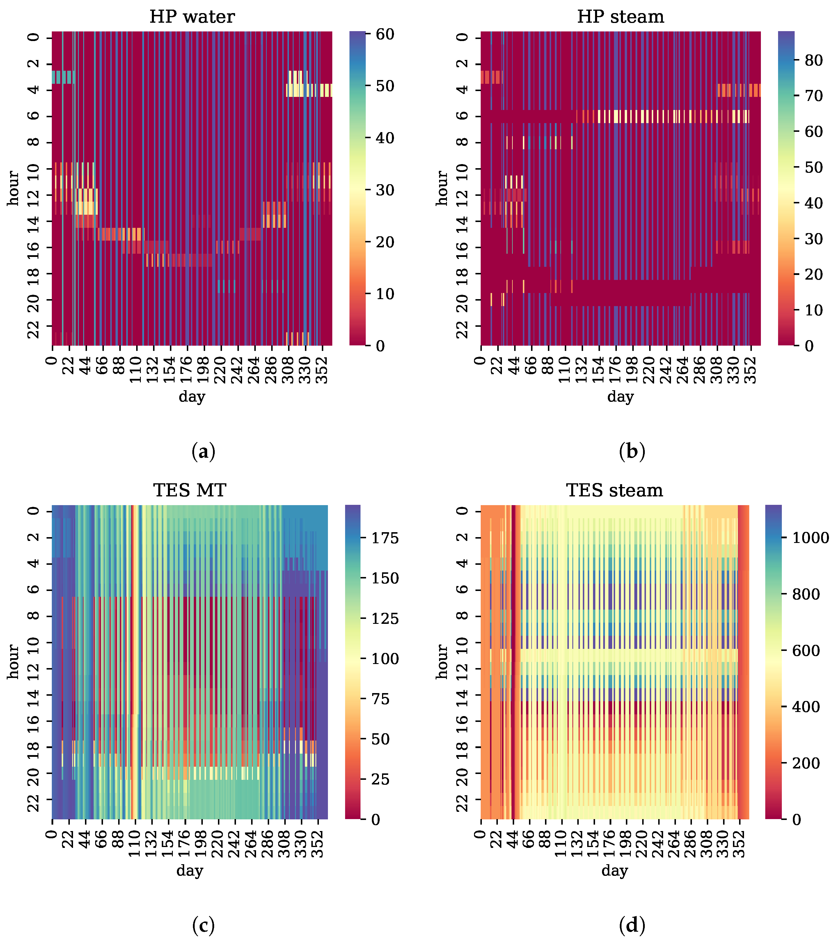
Figure 16 shows heat load profiles for both HPs and the SOC profiles for the medium temperature TES (TES MT) and the steam storage (TES steam). The storages are used for peak shaving to reduce the required sizes of the HPs and other supply units. During non-production days the medium temperature storage is kept at around 70% of its capacity while on brewing days it is fully loaded at night and unloaded at 6 a.m. when the production process starts and heat is required at 90 °C for mashing. At this time, the steam HP is running at part-load or is even turned off. The steam storage shows a similar behavior. On non-production days it is kept on approximately 50% and starts loading at night (around 1 a.m.) and, with varying SOC, satisfies steam demands until 2 p.m., when the storage is completely empty and starts loading to its initial conditions.

The utilization of the CIP tank as a buffer storage for heat supply depends on the implemented decarbonization measures. In the BAU case (Scenario 1), the CIP tank is heated at the exact same time as cleaning is needed in the brewing process and thus potential buffering is not exploited. However, with increasing shares of volatile sources of energy like solar irradiation and the influence of electricity price fluctuations, the capability to act as a storage is increasingly exploited. In Scenario 2 the introduction of a PV system shows that in warm months the CIP tank is heated up on non-production days as cost-free energy is available (Figure 17). Furthermore, as shown in Figure 17b (Scenario 7) the CIP tank is heavily utilized for both inter- and intra-day storage.

The economic potentials for enforced decarbonization rates were also evaluated for the time periods 2025–2030 and 2030–2035. For this purpose Scenarios 2 (no decarbonization enforced), 5 (25% decarbonization), 6 (50% decarbonizaiton), 7 (100% decarbonization), and 8 (no decarbonizaiton enforced, GB reached end of life), which are all based on conditions for 2020–2025, were also optimized with the boundary conditions for 2025–2030 and 2030–2035 (see Table 4). 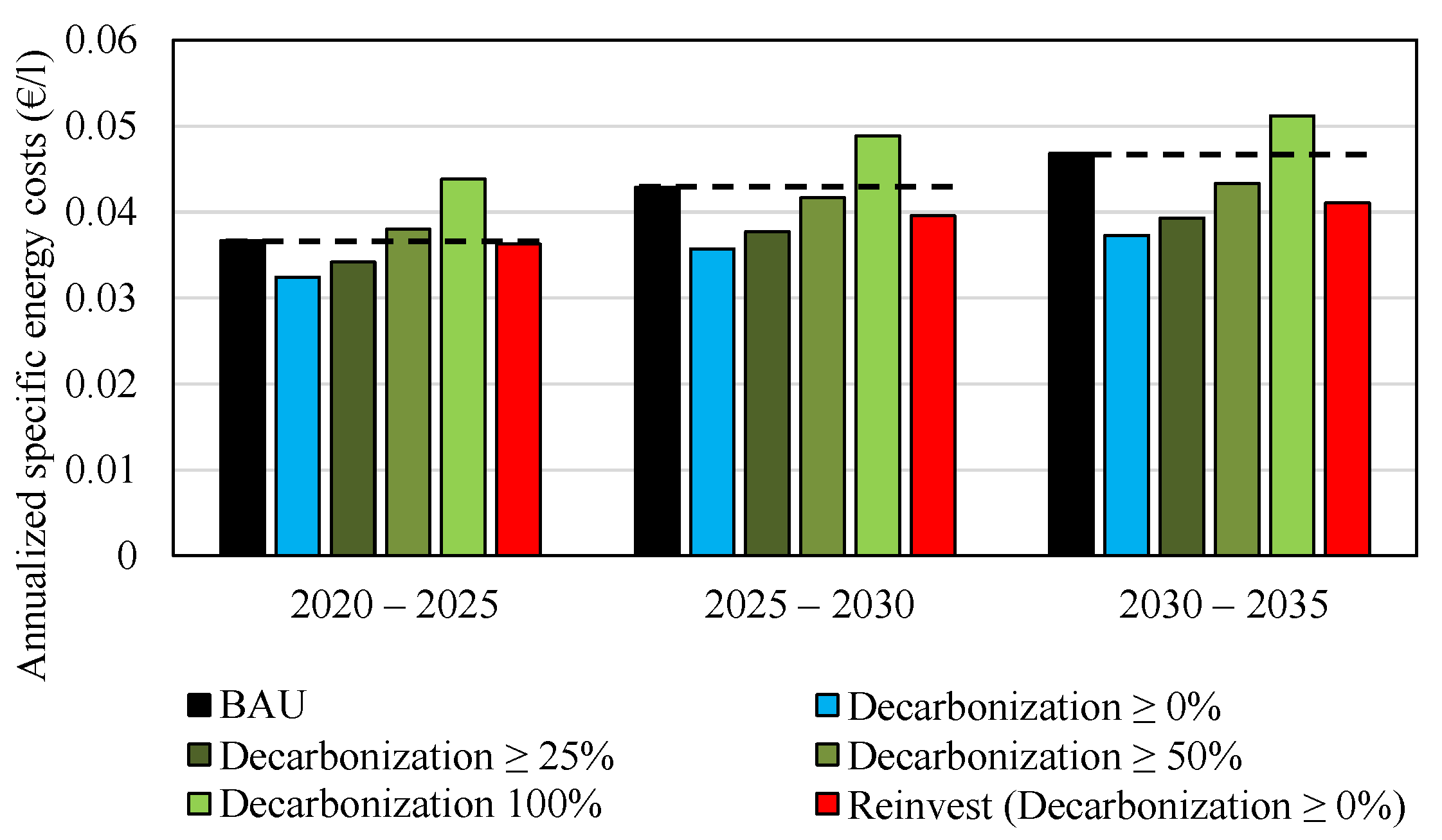Figure 18 summarizes the annualized specific energy costs for beer production for all of these scenarios. Here, annualized specific energy costs are the production output specific total annual costs for energy purchase and annualized investment costs for new energy supply units. The reference for each time period is the expected annualized specific energy costs in the BAU case (dashed lines). For the period 2020–2025 enforcing a 50% reduction in carbon emissions results in an increase in specific energy costs of 3.6%. This shows that even ambitious decarbonization targets of 50% do not result in significant cost premiums, even under current boundary conditions. For the periods 2025–2030 and 2030–2035, solutions with a 50% reduction in CO${}_2$ emissions even have lower annualized specific energy costs compared to the BAU case.

Cost-optimization without enforced emission reduction (Decarbonization ≥ 0) realizes CO${}_2$ reductions of around 6% for the 2020–2025 period with the integration of PV (580 m²), EB (25 kW) and EES (26 kWh). For the 2025–2030 and 2030–2035 periods, no further reduction in emissions was realized. However, cost reductions of 11.6 %, 16.6%, and 20.4% can be realized for the periods 2020–2025, 2025–2030, and 2030–2035, respectively.

These results show that for purely cost-driven optimization, increasing energy and especially CO${}_2$ costs for future scenarios do not lead to significant reductions in emissions even with the relatively long depreciation period of 10 years for investments. However, the results also show that the results for progressive decarbonization rates of 50% and above will compare favorably with the BAU case in terms of annualized energy costs.

5. Conclusions

This article presented a combined method for the optimization of industrial energy systems applied to the use case of a small brewery. The approach simultaneously considered synthesis of the energy supply system and optimization of the heat recovery system and the production schedule and was shown to be suitable to address the process specifics of the underlying case study. Limitations arise with the temporal discretization of hot and cold stream activity as only multiples of the selected interval duration can be considered. Even though the model complexity was acceptable for the small-scale brewery considered in this work, scale-up to more complex industrial energy systems with a large number of heating and cooling requirements and production of multiple batches per day is yet to be examined in future work.

The brewing process under consideration requires electricity supplied by the grid and heat generated by a GB. In the present study, different scenarios considering trends for energy markets and technological developments for the period between 2020 and 2035 were investigated. In the 2020–2025 period, the solution of the purely cost-driven scenario suggests implementing PV, a small EB, and an EES. With increasing energy costs and CO${}_2$ prices, this system combination becomes even more favorable compared to the current energy system in terms of energy costs. However, cost optimization without enforced decarbonization rate results in a mere CO${}_2$ reduction of around 6% as PV substitutes electricity purchase from the grid already assumed to be CO${}_2$ neutral. Optimization of an end-of-life scenario for the GB, which corresponds to a greenfield scenario, leads to the implementation of an additional steam storage but does not change the fact that other potentially renewable supply units like HP are too expensive to be chosen over the GB. However, enforcing decarbonization rates of 25% for the 2020–2025 period results in the implementation of renewable supply units that can match the energy costs of the current energy system. In the 2025–2030 and 2030–2035 periods, enforcing decarbonization rates of 50% and above results in lower costs compared to the current system. In the 2030–2035 period, the gap between the energy costs with the current system and the fully decarbonized energy supply is nearly gone.

Throughout the analysis of the results it became apparent that the current node-based model structure of the energy supply system causes difficulties for interpretation of resulting operation patterns. Here a one-to-one connection between the different units in the energy supply system could facilitate understanding of the system behavior.

References

1. Tollefson, J. COVID curbed carbon emissions in 2020—But not by much. Nature 2021, 589, 343. [Google Scholar] [CrossRef]
2. International Energy Agency. World Energy Outlook 2020; International Energy Agency: Paris, France, 2020. [Google Scholar]
3. Reilly, J.M.; Chen, Y.H.H.; Jacoby, H.D. The COVID-19 effect on the Paris agreement. Humanit. Soc. Sci. Commun. 2021, 8, 16. [Google Scholar] [CrossRef]
4. European Commision. 2030 Climate & Energy Framework; European Commision: Brussels, Belgium, 2021; Available online: https://ec.europa.eu/clima/eu-action/climate-strategies-targets/2030-climate-energy-framework_en (accessed on 24 November 2021).
5. International Energy Agency. CO2 Emissions from Fuel Combustion: Overview; International Energy Agency: Paris, France, 2020. [Google Scholar]
6. Eiholzer, T.; Olsen, D.; Hoffmann, S.; Sturm, B.; Wellig, B. Integration of a solar thermal system in a medium-sized brewery using pinch analysis: Methodology and case study. Appl. Therm. Eng. 2017, 113, 1558–1568. [Google Scholar] [CrossRef]
7. Sturm, B.; Hugenschmidt, S.; Joyce, S.; Hofacker, W.; Roskilly, A.P. Opportunities and barriers for efficient energy use in a medium-sized brewery. Appl. Therm. Eng. 2013, 53, 397–404. [Google Scholar] [CrossRef]
8. Sturm, B.; Butcher, M.; Wang, Y.; Huang, Y.; Roskilly, T. The feasibility of the sustainable energy supply from bio wastes for a small scale brewery—A case study. Appl. Therm. Eng. 2012, 39, 45–52. [Google Scholar] [CrossRef]
9. Lauterbach, C.; Schmitt, B.; Vajen, K. System analysis of a low-temperature solar process heat system. Sol. Energy 2014, 101, 117–130. [Google Scholar] [CrossRef]
10. Muster-Slawitsch, B.; Weiss, W.; Schnitzer, H.; Brunner, C. The green brewery concept—Energy efficiency and the use of renewable energy sources in breweries. Appl. Therm. Eng. 2011, 31, 2123–2134. [Google Scholar] [CrossRef] [Green Version]
11. Dumbliauskaite, M.; Becker, H.; Maréchal, F. Utility optimization in a brewery process based on energy integration methodology. In Proceedings of the 23th International Conference on Efficiency, Cost, Optimization, Simulation and Environmental Impact of Energy Systems, ECOS 2010, Lausanne, Switzerland, 14–17 June 2010; pp. 91–98. [Google Scholar]
12. Frangopoulos, C.A.; Spakovsky, M.R.V.; Sciubba, E. A Brief Review of Methods for the Design and Synthesis Optimization of Energy Systems. Int. J. Appl. Thermodyn. 2002, 5, 151–160. [Google Scholar] [CrossRef]
13. Goderbauer, S.; Comis, M.; Willamowski, F.J. The synthesis problem of decentralized energy systems is strongly NP-hard. Comput. Chem. Eng. 2019, 124, 343–349. [Google Scholar] [CrossRef]
14. Leenders, L.; Bahl, B.; Hennen, M.; Bardow, A. Coordinating scheduling of production and utility system using a Stackelberg game. Energy 2019, 175, 1283–1295. [Google Scholar] [CrossRef]
15. Fathollahi-Fard, A.M.; Woodward, L.; Akhrif, O. Sustainable distributed permutation flow-shop scheduling model based on a triple bottom line concept. J. Ind. Inf. Integr. 2021, 24, 100233. [Google Scholar] [CrossRef]
16. Wang, W.; Zhou, X.; Tian, G.; Fathollahi-Fard, A.M.; Wu, P.; Zhang, C.; Liu, C.; Li, Z. Multi-objective low-carbon hybrid flow shop scheduling via an improved teaching-learning-based optimization algorithm. Sci. Iran. 2022, in press. [Google Scholar] [CrossRef]
17. Fernández, I.; Renedo, C.J.; Pérez, S.F.; Ortiz, A.; Mañana, M. A review: Energy recovery in batch processes. Renew. Sustain. Energy Rev. 2012, 16, 2260–2277. [Google Scholar] [CrossRef]
18. Adonyi, R.; Romero, J.; Puigjaner, L.; Friedler, F. Incorporating heat integration in batch process scheduling. Appl. Therm. Eng. 2003, 23, 1743–1762. [Google Scholar] [CrossRef]
19. Zhao, X.; O’neill, B.; Roach, J.; Wood, R. Heat Integration For Batch Processes: Part 1: Process Scheduling Based on Cascade Analysis. Chem. Eng. Res. Des. 1998, 76, 685–699. [Google Scholar] [CrossRef]
20. Bozan, M.; Borak, F.; Or, I. A computerized and integrated approach for heat exchanger network design in multipurpose batch plants. Chem. Eng. Process. Process Intensif. 2001, 40, 511–524. [Google Scholar] [CrossRef]
21. Chen, C.L.; Chang, C.Y. A resource-task network approach for optimal short-term/periodic scheduling and heat integration in multipurpose batch plants. Appl. Therm. Eng. 2009, 29, 1195–1208. [Google Scholar] [CrossRef]
22. Jung, S.H.; Lee, I.B.; Yang, D.R.; Chang, K.S. Synthesis of maximum energy recovery networks in batch processes. Korean J. Chem. Eng. 1994, 11, 162–171. [Google Scholar] [CrossRef]
23. Lee, B.; Reklaitis, G.V. Optimal Scheduling of Cyclic Batch Processes for Heat Integration—II. Extended Problems. 1995, 19, 907–931. [Google Scholar]
24. Majozi, T. Minimization of energy use in multipurpose batch plants using heat storage: An aspect of cleaner production. J. Clean. Prod. 2009, 17, 945–950. [Google Scholar] [CrossRef] [Green Version]
25. Majozi, T. Heat integration of multipurpose batch plants using a continuous-time framework. Appl. Therm. Eng. 2006, 26, 1369–1377. [Google Scholar] [CrossRef]
26. Stamp, J.; Majozi, T. Optimum heat storage design for heat integrated multipurpose batch plants. Energy 2011, 36, 5119–5131. [Google Scholar] [CrossRef] [Green Version]
27. Magege, S.R.; Majozi, T. A compreHENSive framework for synthesis and design of heat-integrated batch plants: Consideration of intermittently-available streams. Renew. Sustain. Energy Rev. 2021, 135, 110125. [Google Scholar] [CrossRef]
28. Castro, P.M.; Grossmann, I.E.; Zhang, Q. Expanding scope and computational challenges in process scheduling. Comput. Chem. Eng. 2018, 114, 14–42. [Google Scholar] [CrossRef]
29. Pipattanasomporn, M.; Willingham, M.; Rahman, S. Implications of On-Site Distributed Generation for Commercial/Industrial Facilities. IEEE Trans. Power Syst. 2005, 20, 206–212. [Google Scholar] [CrossRef]
30. Paudyal, S.; Canizares, C.A.; Bhattacharya, K. Optimal Operation of Industrial Energy Hubs in Smart Grids. IEEE Trans. Smart Grid 2015, 6, 684–694. [Google Scholar] [CrossRef]
31. Atabay, D. An open-source model for optimal design and operation of industrial energy systems. Energy 2017, 121, 803–821. [Google Scholar] [CrossRef]
32. Wilkendorf, F.; Espuña, A.; Puigjaner, L. Minimization of the annual cost for complete utility systems. Chem. Eng. Res. Des. 1998, 76, 239–245. [Google Scholar] [CrossRef]
33. Voll, P.; Klaffke, C.; Hennen, M.; Bardow, A. Automated superstructure-based synthesis and optimization of distributed energy supply systems. Energy 2013, 50, 374–388. [Google Scholar] [CrossRef]
34. Larsson, M.; Wang, C.; Dahl, J. Development of a method for analysing energy, environmental and economic efficiency for an integrated steel plant. Appl. Therm. Eng. 2006, 26, 1353–1361. [Google Scholar] [CrossRef]
35. Klugman, S.; Karlsson, M.; Moshfegh, B. Modeling an industrial energy system: Perspectives on regional heat cooperation. Int. J. Energy Res. 2008, 32, 793–807. [Google Scholar] [CrossRef]
36. Thollander, P.; Mardan, N.; Karlsson, M. Optimization as investment decision support in a Swedish medium-sized iron foundry—A move beyond traditional energy auditing. Appl. Energy 2009, 86, 433–440. [Google Scholar] [CrossRef] [Green Version]
37. Karlsson, M. The MIND method: A decision support for optimization of industrial energy systems—Principles and case studies. Appl. Energy 2011, 88, 577–589. [Google Scholar] [CrossRef] [Green Version]
38. Hawkes, A.D.; Leach, M.A. Modelling high level system design and unit commitment for a microgrid. Appl. Energy 2009, 86, 1253–1265. [Google Scholar] [CrossRef]
39. Zidan, A.; Gabbar, H.A.; Eldessouky, A. Optimal planning of combined heat and power systems within microgrids. Energy 2015, 93, 235–244. [Google Scholar] [CrossRef]
40. Brandoni, C.; Renzi, M. Optimal sizing of hybrid solar micro-CHP systems for the household sector. Appl. Therm. Eng. 2015, 75, 896–907. [Google Scholar] [CrossRef]
41. Wouters, C.; Fraga, E.S.; James, A.M. An energy integrated, multi-microgrid, MILP (mixed-integer linear programming) approach for residential distributed energy system planning—A South Australian case-study. Energy 2015, 85, 30–44. [Google Scholar] [CrossRef] [Green Version]
42. Fuentes-Cortés, L.F.; Ponce-Ortega, J.M.; Nápoles-Rivera, F.; Serna-González, M.; El-Halwagi, M.M. Optimal design of integrated CHP systems for housing complexes. Energy Convers. Manag. 2015, 99, 252–263. [Google Scholar] [CrossRef]
43. Rieder, A.; Christidis, A.; Tsatsaronis, G. Multi criteria dynamic design optimization of a small scale distributed energy system. Energy 2014, 74, 230–239. [Google Scholar] [CrossRef]
44. Wang, H.; Yin, W.; Abdollahi, E.; Lahdelma, R.; Jiao, W. Modelling and optimization of CHP based district heating system with renewable energy production and energy storage. Appl. Energy 2015, 159, 401–421. [Google Scholar] [CrossRef]
45. Mehleri, E.D.; Sarimveis, H.; Markatos, N.C.; Papageorgiou, L.G. A mathematical programming approach for optimal design of distributed energy systems at the neighbourhood level. Energy 2012, 44, 96–104. [Google Scholar] [CrossRef]
46. Chen, C.L.; Li, P.Y.; Chen, H.C.; Lee, J.Y. Synthesis of transcritical ORC-integrated heat exchanger networks for waste heat recovery. In 12th International Symposium on Process Systems Engineering and 25th European Symposium on Computer Aided Process Engineering; Elsevier: Amsterdam, The Netherlands, 2015; Volume 37, pp. 1073–1078. [Google Scholar] [CrossRef]
47. Goh, W.S.; Wan, Y.K.; Tay, C.K.; Ng, R.T.; Ng, D.K. Automated targeting model for synthesis of heat exchanger network with utility systems. Appl. Energy 2016, 162, 1272–1281. [Google Scholar] [CrossRef]
48. Huang, X.; Lu, P.; Luo, X.; Chen, J.; Yang, Z.; Liang, Y.; Wang, C.; Chen, Y. Synthesis and simultaneous MINLP optimization of heat exchanger network, steam Rankine cycle, and organic Rankine cycle. Energy 2020, 195, 116922. [Google Scholar] [CrossRef]
49. Liu, F.; Ma, J.; Feng, X.; Wang, Y. Simultaneous integrated design for heat exchanger network and cooling water system. Appl. Therm. Eng. 2018, 128, 1510–1519. [Google Scholar] [CrossRef]
50. Martelli, E.; Elsido, C.; Mian, A.; Marechal, F. MINLP model and two-stage algorithm for the simultaneous synthesis of heat exchanger networks, utility systems and heat recovery cycles. Comput. Chem. Eng. 2017, 106, 663–689, ESCAPE-26. [Google Scholar] [CrossRef]
51. Elsido, C.; Cremonesi, A.; Martelli, E. A novel sequential synthesis algorithm for the integrated optimization of Rankine cycles and heat exchanger networks. Appl. Therm. Eng. 2021, 192, 116594. [Google Scholar] [CrossRef]
52. Hofmann, R.; Panuschka, S.; Beck, A. A simultaneous optimization approach for efficiency measures regarding design and operation of industrial energy systems. Comput. Chem. Eng. 2019, 128, 246–260. [Google Scholar] [CrossRef]
53. Elsido, C.; Martelli, E.; Grossmann, I.E. Multiperiod optimization of heat exchanger networks with integrated thermodynamic cycles and thermal storages. Comput. Chem. Eng. 2021, 149, 107293. [Google Scholar] [CrossRef]
54. Halmschlager, D.; Beck, A.; Knöttner, S.; Koller, M.; Hofmann, R. Combined optimization for retrofitting of heat recovery and thermal energy supply in industrial systems. Appl. Energy 2022, 305, 117820. [Google Scholar] [CrossRef]
55. Yee, T.F.; Grossmann, I.E. Simultaneous optimization models for heat integration—II. Heat exchanger network synthesis. Comput. Chem. Eng. 1990, 14, 1165–1184. [Google Scholar] [CrossRef]
56. Beck, A.; Hofmann, R. A Novel Approach for Linearization of a MINLP Stage-Wise Superstructure Formulation. Comput. Chem. Eng. 2018, 112, 17–26. [Google Scholar] [CrossRef]
57. Morales-España, G.; Gentile, C.; Ramos, A. Tight MIP formulations of the power-based unit commitment problem. OR Spectr. 2015, 37, 929–950. [Google Scholar] [CrossRef]
58. Kotzur, L.; Markewitz, P.; Robinius, M.; Stolten, D. Time series aggregation for energy system design: Modeling seasonal storage. Appl. Energy 2018, 213, 123–135. [Google Scholar] [CrossRef] [Green Version]
59. Castro, P.; Barbosa-Póvoa, A.; Matos, H. An improved RTN continuous-time formulation for the short-term scheduling of multipurpose batch plants. Ind. Eng. Chem. Res. 2001, 40, 2059–2068. [Google Scholar] [CrossRef]
60. Hegyhati, M.; Friedler, F. Overview of Industrial Batch Process Scheduling. Chem. Eng. Trans. 2010, 21, 895–900. [Google Scholar] [CrossRef]
61. ASHRAE Handbook: Heating, Ventilating, and Air-Conditioning Applications; American Society of Heating, Refrigerating and Air Conditioning Engineers: Atlanta, GA, USA, 2003.
62. ISO 9806:2017(en); Solar Energy—Solar Thermal Collectors—Test Methods. International Organization for Standardization: Geneva, Switzerland, 2017.
63. van der Heijde, B.; Vandermeulen, A.; Salenbien, R.; Helsen, L. Representative days selection for district energy system optimisation: A solar district heating system with seasonal storage. Appl. Energy 2019, 248, 79–94. [Google Scholar] [CrossRef]
64. Aktuelle meteorologische Messwerte; Universität für Bodenkultur Wien: Vienna, Austria, 2021.
65. EXAA-Marktdaten—Historische Daten: 2019; Energy Exchange Austria: Vienna, Austria, 2021.
66. Klima- und Energiefonds. Leitfaden Photovoltaik–Anlagen. Vienna, Austria, 2021. Available online: https://www.klimafonds.gv.at/call/photovoltaik-anlagen-2022/ (accessed on 24 November 2021).
67. Goverment of Upper Austria. Förderungen zum Thema Umwelt und Natur. Linz, Austria, 2021. Available online: https://www.land-oberoesterreich.gv.at/12846.htm (accessed on 24 November 2021).
68. Huneke, F.; Perez-Linkenheil, C.; Heidinger, P. Österreichs Weg Richtung 100% Erneuerbare. Eine Analyse von 2013 Mit Ausblick 2050; Energy Brainpool: Berlin, Germany, 2019. [Google Scholar]
69. International Energy Agency. Cumulative Capacity and Capital Cost Index Learning Curve for Vapour Compression Applications in the Sustainable Development Scenario, 2019–2070; International Energy Agency: Paris, France, 2020. [Google Scholar]
70. IRENA. Future of Solar Photovoltaic: Deployment, Investment, Technology, Grid Integration and Socio-Economic Aspects (A Global Energy Transformation: Paper); IRENA: Abu Dhabi, United Arab Emirates, 2019. [Google Scholar]
71. Brauerei Müggelland. Online Forum Post—Thermische Bottichmasse Bestimmen, 27 March 2018. Available online: https://brauerei.mueggelland.de/forum/topic/43.html (accessed on 24 November 2021).
72. Muster-Slawitsch, B.; Hubmann, M.; Murkovic, M.; Brunner, C. Process modelling and technology evaluation in brewing. Chem. Eng. Process. Process Intensif. 2014, 84, 98–108. [Google Scholar] [CrossRef]
73. Scheer, F. Thermal Process Engineering for Brewers (Presentation Material), Franklin, WI, USA, 24 October 2014. Available online: https://www.mbaa.com/districts/NorthernCalifornia/Documents/2014%20Joint%20Technical%20Conference/3-3%20F%20Scheer%20Thermodynamics%20for%20Brewers.pdf (accessed on 24 November 2021).
Figure 1. Structure of the proposed optimization model and the interfaces between the individual sub-models highlighted in dark grey.
Processes 10 00572 g001
Figure 2. Resulting schedule for example case with and without heat recovery—(heating: blue, cooling: red, power: grey).
Processes 10 00572 g002
Figure 3. Mapping of representative days for storage SOC calculations.
Processes 10 00572 g003
Figure 4. Supply superstructure and overview of brewing process.
Processes 10 00572 g004
Figure 5. Mapping of representative days (white: weekends, grey: weekdays without production, black: production days).
Processes 10 00572 g005
Figure 6. Resulting profiles after mapping for (a) electricity prices and (b) electricity base demand.
Processes 10 00572 g006
Figure 7. Size of all considered units for each scenario.
Processes 10 00572 g007
Figure 8. Investment costs for units in the cost optimal solution and minimal required cost reduction Δ C m i n for units to be considered in the cost optimal solution.
Processes 10 00572 g008
Figure 9. Existing HEN (black) and reuse of HEX in Scenarios 5–7 for heat supply via hot water (grey).
Processes 10 00572 g009
Figure 10. Optimized production schedule for all scenarios indicating different requirements (heating: blue, cooling: red, power: grey).
Processes 10 00572 g010
Figure 11. Energy flows in the energy supply system for the BAU scenario (Scenario 1).
Processes 10 00572 g011
Figure 12. (a) Heat load of GB in kW and (b) SOC of brewing water tank in kWh (all Scenario 1).
Processes 10 00572 g012
Figure 13. Energy flows in the energy supply system for Scenario 2.
Processes 10 00572 g013
Figure 14. (a) Power generation of PV in kW, (b) SOC of EES in kWh, and (c) heat load of EB in kW (all Scenario 2).
Processes 10 00572 g014
Figure 15. Energy flows in the energy supply system for Scenario 7.
Processes 10 00572 g015
Figure 16. (a) Heat load of HP water in kW, (b) heat load of HP steam in kW, (c) SOC of TES MT in kWh, and (d) SOC of TES steam in kWh (all Scenario 7).
Processes 10 00572 g016
Figure 17. SOC of the CIP tank in kWh (a) Scenario 2 (b) Scenario 7.
Processes 10 00572 g017
Figure 18. Annualized energy costs per liter beer for various enforced decarbonization rates.
Processes 10 00572 g018