
Synthesizing Electrically Equivalent Circuits for Use in Electrochemical Impedance Spectroscopy through Grammatical Evolution

 ,
,  , ,
, , 
Abstract
:1. Introduction
2. Grammatical Evolution
2.1. The Grammar
2.2. Mapping Process Examples
2.2.1. A Single Element Example
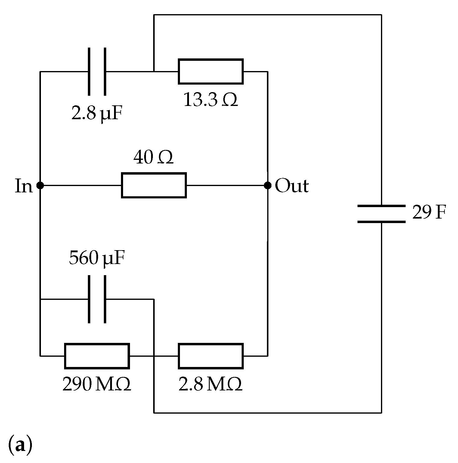
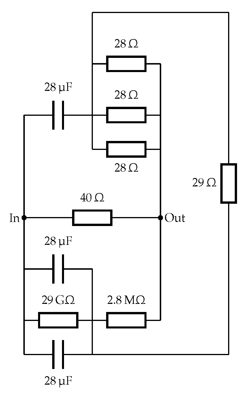
2.2.2. A Complete Netlist
2.3. Genetic Operations and Circuits
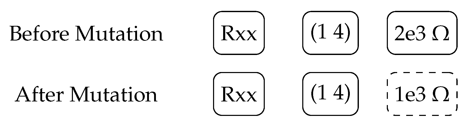
2.3.1. Circuit Mutation
2.3.2. Circuit Crossover
3. Experiments and Data
3.1. Objective Function and Evaluation
Sheppard’s Objective Function
3.2. Data Sets Used for Evaluation
3.2.1. Randles Circuits
3.2.2. Cole–Cole Model
3.2.3. Solid Oxide Fuel Cell Data
4. Results
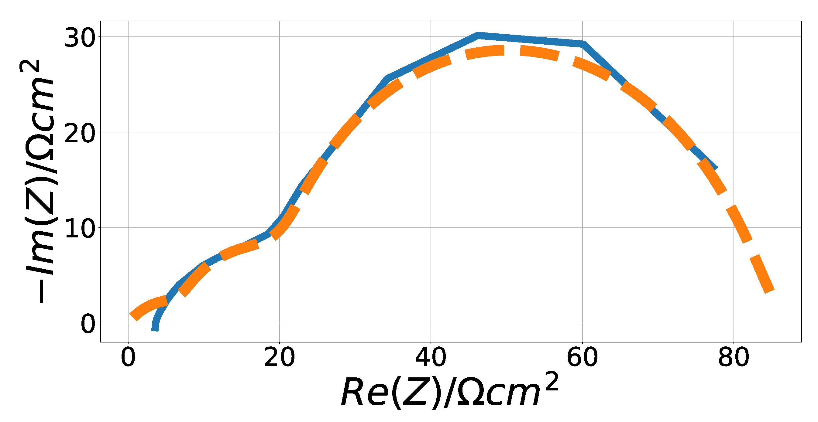
4.1. Randles Impedance Characteristic Matching
4.2. Cole–Cole Fitting
4.3. Solid Oxide Fuel Cell Fitting
5. Discussion
Author Contributions
Funding
Institutional Review Board Statement
Informed Consent Statement
Data Availability Statement
Acknowledgments
Conflicts of Interest
References
- Barsoukov, E.; Macdonald, J.R. Impedance Spectroscopy: Theory, Experiment, and Applications; Wiley: Hoboken, NJ, USA, 2005. [Google Scholar]
- Yuan, X.Z.; Song, C.; Wang, H.; Zhang, J. EIS Applications. In Electrochemical Impedance Spectroscopy in PEM Fuel Cells: Fundamentals and Applications; Springer: London, UK, 2010; pp. 263–345. [Google Scholar] [CrossRef]
- Wan, T.H.; Saccoccio, M.; Chen, C.; Ciucci, F. Influence of the Discretization Methods on the Distribution of Relaxation Times Deconvolution: Implementing Radial Basis Functions with DRTtools. Electrochim. Acta 2015, 184, 483–499. [Google Scholar] [CrossRef]
- Dion, F.; Lasia, A. The use of regularization methods in the deconvolution of underlying distributions in electrochemical processes. J. Electroanal. Chem. 1999, 475, 28–37. [Google Scholar] [CrossRef]
- Zic, M.; Pereverzyev, S., Jr.; Subotic, V.; Pereverzyev, S. Adaptive multi-parameter regularization approach to construct the distribution function of relaxation times. Gem-Int. J. Geomath. 2020, 11, 1–23. [Google Scholar] [CrossRef] [Green Version]
- Song, J.; Bazant, M. Electrochemical Impedance Imaging via the Distribution of Diffusion Times. Phys. Rev. Lett. 2018, 120, 116001. [Google Scholar] [CrossRef] [PubMed] [Green Version]
- Pereverzev, S.V.; Solodky, S.G.; Vasylyk, V.B.; Žic, M. Regularized Collocation in Distribution of Diffusion Times Applied to Electrochemical Impedance Spectroscopy. Comput. Methods Appl. Math. 2020, 20, 517–530. [Google Scholar] [CrossRef]
- Boukamp, B.A. A nonlinear least-squares fit procedure for analysis of immittance data of electrochemical systems. Solid State Ionics 1986, 20, 31–44. [Google Scholar] [CrossRef] [Green Version]
- Macdonald, J.R.; Schoonman, J.; Lehnen, A.P. The applicability and power of complex non-linear least-squares for the analysis of impedance and admittance data. J. Electroanal. Chem. 1982, 131, 77–95. [Google Scholar] [CrossRef]
- Sihvo, J.; Roinila, T.; Stroe, D.I. Novel Fitting Algorithm for Parametrization of Equivalent Circuit Model of Li-Ion Battery from Broadband Impedance Measurements. IEEE Trans. Ind. Electron. 2021, 68, 4916–4926. [Google Scholar] [CrossRef]
- Žic, M. An alternative approach to solve complex nonlinear least-squares problems. J. Electroanal. Chem. 2016, 760, 85–96. [Google Scholar] [CrossRef]
- Kobayashi, K.; Suzuki, T. Development of impedance analysis software implementing a support function to find good initial guess using an interactive graphical user interface. Electrochemistry 2020, 88, 39–44. [Google Scholar] [CrossRef] [Green Version]
- Žic, M.; Subotić, V.; Pereverzyev, S.; Fajfar, I. Solving CNLS problems using Levenberg-Marquardt algorithm: A new fitting strategy combining limits and a symbolic Jacobian matrix. J. Electroanal. Chem. 2020, 866, 114171. [Google Scholar] [CrossRef]
- Lan, C.; Liao, Y.; Hu, G. A unified equivalent circuit and impedance analysis method for galloping piezoelectric energy harvesters. Mech. Syst. Signal Process. 2022, 165, 108339. [Google Scholar] [CrossRef]
- Zic, M. Optimizing Noisy CNLS Problems by Using the Adaptive Nelder-Mead Algorithm: A New Approach to Escape from Local Minima. 2018. Available online: https://ricamwww.ricam.oeaw.ac.at/files/reports/18/rep18-22.pdf (accessed on 19 October 2021).
- Levenberg, K. A method for the solution of certain non-linear problems in least squares. Q. Appl. Math. 1944, 2, 164–168. [Google Scholar] [CrossRef] [Green Version]
- Marquardt, D.W. An algorithm for least-squares estimation of nonlinear parameters. J. Soc. Ind. Appl. Math. 1963, 11, 431–441. [Google Scholar] [CrossRef]
- Moré, J. The Levenberg-Marquardt algorithm: Implementation and theory. In Numerical Analysis; Lecture Notes in Mathematics; Watson, G., Ed.; Springer: Berlin/Heidelberg, Germany, 1978; Volume 630, pp. 105–116. [Google Scholar] [CrossRef] [Green Version]
- Nelder, J.A.; Mead, R. A Simplex Method for Function Minimization. Comput. J. 1965, 7, 308–313. [Google Scholar] [CrossRef]
- Dellis, J.L.; Carpentier, J.L. Nelder and Mead algorithm in impedance spectra fitting. Solid State Ionics 1993, 62, 119–123. [Google Scholar] [CrossRef]
- Kunaver, M. Grammatical Evolution-based Analog Circuit Synthesis. Inf. MIDEM 2019, 49, 229–239. [Google Scholar]
- O’Neil, M.; Ryan, C. Grammatical Evolution. In Grammatical Evolution: Evolutionary Automatic Programming in an Arbitrary Language; Springer: Boston, MA, USA, 2003; pp. 33–47. [Google Scholar] [CrossRef]
- Macdonald, J.R. Impedance spectroscopy: Models, data fitting, and analysis. Solid State Ionics 2005, 176, 1961–1969. [Google Scholar] [CrossRef]
- Tuinenga, P.W. SPICE: A Guide to Circuit Simulation and Analysis Using PSpice, 1st ed.; Prentice Hall: Englewood Cliffs, NJ, USA, 1988. [Google Scholar]
- Kunaver, M.; Fajfar, I. Grammatical Evolution in a Matrix Factorization Recommender System. In International Conference on Artificial Intelligence and Soft Computing; Rutkowski, L., Korytkowski, M., Scherer, R., Tadeusiewicz, R., Zadeh, L.A., Zurada, J.M., Eds.; Lecture Notes in Computer Science; Springer: Berlin/Heidelberg, Germany, 2016; Volume 9692, pp. 392–400. [Google Scholar] [CrossRef]
- Naur, P. Revised Report on the Algorithmic Language Algol 60. Commun. ACM 1963, 6, 1–23. [Google Scholar]
- Sheppard, R.J.; Jordan, B.P.; Grant, E.H. Least squares analysis of complex data with applications to permittivity measurements. J. Phys. D Appl. Phys. 1970, 3, 1759–1764. [Google Scholar] [CrossRef]
- Zoltowski, P. The error function for fitting of models to immittance data. J. Electroanal. Chem. 1984, 178, 11–19. [Google Scholar] [CrossRef]
- Cole, K.S.; Cole, R.H. Dispersion and absorption in dielectrics I. Alternating current characteristics. J. Chem. Phys. 1941, 9, 341–351. [Google Scholar] [CrossRef] [Green Version]
- Žic, M.; Fajfar, I.; Subotić, V.; Pereverzyev, S.; Kunaver, M. Investigation of Electrochemical Processes in Solid Oxide Fuel Cells by Modified Levenberg–Marquardt Algorithm: A New Automatic Update Limit Strategy. Processes 2021, 9, 108. [Google Scholar] [CrossRef]
- Subotić, V.; Stoeckl, B.; Lawlor, V.; Strasser, J.; Schroettner, H.; Hochenauer, C. Towards a practical tool for online monitoring of solid oxide fuel cell operation: An experimental study and application of advanced data analysis approaches. Appl. Energy 2018, 222, 748–761. [Google Scholar] [CrossRef]


| Nonterminal | Expands to |
|---|---|
| <netlist> | twelve space separated <part> nonterminals |
| <part> | <res> | <cap> | <zarc> | None |
| <res> | rXX (<gpair>) <num><num>e<exp> |
| <cap> | cXX (<gpair>) <num><num>e-<exp> |
| <zarc> | aXX (<gpair>) zarcX .model zarcY zarc |
| (r=<num>e<exp> | |
| tau=<num>e-<zexp>n=0.<znum><num>) | |
| <num> | 1 | 2 | 3 | 4 | 5 | 6 | 7 | 8 | 9 | 0 |
| <exp> | 0 | 3 | 6 | 9 | 12 |
| <zexp> | 1 | 2 | 3 | 4 | 5 |
| <znum> | 5 | 6 | 7 | 8 | 9 |
| <gpair> | input 1 | input 2 | input 3 | input 4 | input output | |
| 1 2 | 1 3 | 1 4 | 1 output | | |
| 2 3 | 2 4 | 2 output | | |
| 3 4 | 3 output | | |
| 4 output |
| Parameter | Value Range |
|---|---|
| Resistance | [1 , 99 T] |
| Capacitance | [99 pF, 99 F] |
| ZARC resistance | [1 , 9 T] |
| ZARC n factor | [, ] |
| ZARC time constant | [ s, s] |
| Number of Rules/ | Selected | ||
|---|---|---|---|
| Codon | Nonterminal | Resulting Rule | Terminal |
| 12 | <part> | 4/0 | <res> |
| 127 | <gpair> | 15/7 | 1 4 |
| 209 | <num> | 10/9 | 0 |
| 21 | <num> | 10/1 | 2 |
| 76 | <exp> | 5/1 | 3 |
| 236 | 143 | 231 | 47 | 145 | 125 | 33 | 201 | 237 | 187 | 180 |
| 104 | 251 | 217 | 172 | 112 | 143 | 31 | 227 | 45 | 228 | 183 |
| 101 | 218 | 83 | 152 | 4 | 253 | 220 | 215 | 77 | 183 | 51 |
| 147 | 32 | 220 | 173 | 31 | 177 | 0 | 113 | 30 | 211 | 157 |
| 212 | 45 | 22 | 201 | 117 | 230 | 223 | 171 | 89 | 143 | 243 |
| 135 | 135 | 11 | 37 | 178 | 161 | 139 | 191 | 148 | 208 | 219 |
| 159 | 200 | 196 | 231 | 252 | 254 | 232 | 183 | 119 | 165 | 156 |
| 219 | 205 | 138 | 254 | 133 | 123 | 96 | 68 | 204 | 77 | 229 |
| 114 | 116 | 139 | 219 | 189 | 97 | 32 | 101 | 166 | 140 | 98 |
| 168 | 220 | 198 | 93 | 146 | 129 | 130 | 194 | 6 | 125 | 236 |
| 32 | 51 | 68 | 20 | 183 | 249 | 96 | 156 | 28 | 12 | 62 |
| 104 | 253 | 104 | 174 | 65 | 11 | 185 | 37 | 137 | 26 | 238 |
| 86 | 103 | 58 | 122 | 110 | 80 | 222 | 83 | 125 | 18 | 163 |
| 73 | 19 | 255 | 85 | 104 | 149 | 105 | 127 | 189 | 218 | 54 |
| 198 | 183 | 144 | 162 | 161 | 47 | 77 | 56 | 21 | 9 | 15 |
| 16 | 66 | 34 | 132 | 101 | 150 | 135 | 192 | 184 | 138 | 134 |
| 96 | 96 | 183 | 212 | 147 | 3 | 196 | 101 | 246 | 9 | 241 |
| 156 | 109 | 113 | 254 | 115 | 13 | 35 | 48 | 117 | 65 | 141 |
| 8 | 21 | 229 | 74 | 100 | 222 | 69 | 23 | 90 | 7 | 42 |
| 168 | 120 | 227 | 206 | 147 | 139 | 190 | 22 | 127 | 148 | 187 |
| 45 | 235 | 97 | 36 | 192 | 92 | 254 | 64 | 188 | 247 | 51 |
| 183 | 194 | 164 | 61 | 121 | 188 | 100 | 58 | 226 | 255 | 137 |
| 16 | 88 | 223 | 148 | 155 | 225 | 28 | 233 | 120 | 222 | 167 |
| 246 | 216 | 225 | 163 | 2 | 86 | 52 | 189 | 45 | 232 | 159 |
| 118 | 165 | 172 | 74 | 151 | 80 | 19 | 219 | 141 | 0 | 22 |
| 129 | 33 | 190 | 184 | 253 | 248 | 205 | 30 | 186 | 6 | 186 |
| 84 | 71 | 126 | 199 | 133 | 127 | 180 | 172 | 159 | 166 | 71 |
| 27 | 105 | 189. |
| Parameter | Description |
|---|---|
| Population Size | 300 |
| Generations | 250 |
| Mutation type | Fixed Mutation probability |
| Mutation chance | 5% |
| Fitness | Sheppard’s Objective Function |
| Elitism | Best individual always survives |
| Elite size | 60% of population |
| Synthetic Data | ||||||
|---|---|---|---|---|---|---|
| ZARC | 50 | 0.01 | 0.7 | 50 | 0.0001 | 0.7 |
| Element | n | ||
|---|---|---|---|
| ZARC1 | 348.21 | 0.0003 | 0.91 |
| ZARC2 | 65 | 0.065 | 0.53 |
| ZARC3 | 66 | 0.003 | 0.57 |
| ZARC4 | 80 | 0.00005 | 0.5 |
Publisher’s Note: MDPI stays neutral with regard to jurisdictional claims in published maps and institutional affiliations. |
© 2021 by the authors. Licensee MDPI, Basel, Switzerland. This article is an open access article distributed under the terms and conditions of the Creative Commons Attribution (CC BY) license (https://creativecommons.org/licenses/by/4.0/).
Share and Cite
Kunaver, M.; Žic, M.; Fajfar, I.; Tuma, T.; Bűrmen, Á.; Subotić, V.; Rojec, Ž. Synthesizing Electrically Equivalent Circuits for Use in Electrochemical Impedance Spectroscopy through Grammatical Evolution. Processes 2021, 9, 1859. https://doi.org/10.3390/pr9111859
Kunaver M, Žic M, Fajfar I, Tuma T, Bűrmen Á, Subotić V, Rojec Ž. Synthesizing Electrically Equivalent Circuits for Use in Electrochemical Impedance Spectroscopy through Grammatical Evolution. Processes. 2021; 9(11):1859. https://doi.org/10.3390/pr9111859
Chicago/Turabian StyleKunaver, Matevž, Mark Žic, Iztok Fajfar, Tadej Tuma, Árpád Bűrmen, Vanja Subotić, and Žiga Rojec. 2021. "Synthesizing Electrically Equivalent Circuits for Use in Electrochemical Impedance Spectroscopy through Grammatical Evolution" Processes 9, no. 11: 1859. https://doi.org/10.3390/pr9111859
APA StyleKunaver, M., Žic, M., Fajfar, I., Tuma, T., Bűrmen, Á., Subotić, V., & Rojec, Ž. (2021). Synthesizing Electrically Equivalent Circuits for Use in Electrochemical Impedance Spectroscopy through Grammatical Evolution. Processes, 9(11), 1859. https://doi.org/10.3390/pr9111859