Parameter Identification of a Quasi-3D PEM Fuel Cell Model by Numerical Optimization

Abstract

Polymer electrolyte membrane fuel cells (PEMFCs) supplied with green hydrogen from renewable sources are a promising technology for carbon dioxide-free energy conversion. Many mathematical models to describe and understand the internal processes have been developed to design more powerful and efficient PEMFCs. Parameterizing such models is challenging, but indispensable to predict the species transport and electrochemical conversion accurately. Many material parameters are unknown, or the measurement methods required to determine their values are expensive, time-consuming, and destructive. This work shows the parameterization of a quasi-3D PEMFC model using measurements from a stack test stand and numerical optimization algorithms. Differential evolution and the Nelder–Mead simplex algorithm were used to optimize eight material parameters of the membrane, cathode catalyst layer (CCL), and gas diffusion layer (GDL). Measurements with different operating temperatures and gas inlet pressures were available for optimization and validation. Due to the low operating temperature of the stack, special attention was paid to the temperature dependent terms in the governing equations. Simulations with optimized parameters predicted the steady-state and transient behavior of the stack well. Therefore, valuable data for the characterization of the membrane, the CCL and GDL was created that can be used for more detailed CFD simulations in the future.

1. Introduction

Ongoing climate change and the need to reduce greenhouse gas emissions require new technologies to meet global energy needs with renewable sources. Polymer electrolyte membrane fuel cells (PEMFCs) powered by green hydrogen show a performance that is well suited for automotive applications due to their high power density, high efficiency, and high startup availability [1]. However, due to the low operating temperatures, water management is a challenge. On the one hand, sufficient hydration of the membrane must be ensured for proper conduction of hydrogen ions, and on the other hand, flooding of the microporous layers and GDLs must be avoided.

Mathematical models have been developed to better understand the internal processes, such as the formation of liquid water and its transport, and to design more efficient and powerful fuel cells (FCs). In addition, predictive and reliable models are used to forecast the internal conditions and optimize their operation strategy, e.g., optimization of purging strategy due to nitrogen and water accumulation in the anode [2]. Therefore, the parameterization of the models is crucial. The processes and chemical reactions inside a fuel cell depend on many physical phenomena such as mass/heat/charge transport and electrochemistry. The available models can be categorized in [3,4]: (1) the degree of physical modeling (analytical, (semi-)empirical, mechanistic) and (2) the spatial resolution of the models (0D, 1D, 2D, quasi 3D, 3D). Springer [5] developed one of the first 1D semi-empirical models for the hydration of the membrane. The work of Bernardi and Verbrugge [6] is considered as one of the cornerstones in the development of mechanistic models. The models developed at the beginning of fuel cell modeling were mostly reduced to 0D or 1D [5,7,8,9], whereas more recent models are extended to 2D [10,11], quasi-3D [12,13,14,15], and 3D(-CFD) [16,17,18].

The required model parameters of full mechanistic models are physical quantities and fundamental constants to describe the transport of momentum, species, heat and electric charge, electrochemistry, and geometry. Complex and expensive measurements, expert knowledge, and other data sources such as scientific literature and datasheets are required to parameterize the numerous submodels of spatially resolved approaches, like the agglomerate model for CLs and gas diffusion models for membranes. Moreover, anisotropic material parameters for porous media (CL, GDL) or graphite BPP, as well as their dependence on the cells’ clamping force, further increase unknown material parameters. Therefore, in addition to measurements, simpler models such as 1D, 2D, or quasi-3D can be applied to obtain some of these parameters and thus reduce the number of unknowns. They are faster than computationally intensive CFD models but have similar physical behavior. Many evaluations can be performed quickly with these models, e.g., for numerical optimization of parameters with available comparison data.

As pointed out by Demuren and Edwards [4] and d’Adamo et al. [19], the detailed measurements to determine the geometric, chemical, and physical characteristics of the PEMFCs’ materials is a complex and time-consuming task. In addition, many of the measurement methods are ex situ and even destructive. Additional difficulties must be overcome if novel materials like ultra-thin membranes with reinforced short-side-chain PFSA, typical for modern automotive applications, are used. Dickinson and Smith [20] pointed out that there is a lack of information in the scientific literature for models and material properties for other PFSAs than Nafion^®. However, the models developed for Nafion^® 117/125 have been frequently used and showed promising results [12,20,21].

To get a first overview of the influence of model and material parameters on the performance of a PEMFC, Karpenko-Jereb et al. [22] conducted a study on the impact of parameters using a 3D CFD model. They showed that reference exchange current density (RECD), the transfer coefficient, the ionic conductivity, and the porosity of the GDL have the biggest influence on the simulated current density. Another possibility to determine the main influencing parameters of a mathematical model is a sensitivity analysis. Vetter and Schumacher [23] made a comprehensive sensitivity analysis of a macro-homogeneous, steady-state, two-phase flow model. They showed that the three most influential parameters of their model on fuel cell performance are membrane properties: the diffusion coefficient of water in ionomer, the ionic conductivity, and the electro-osmotic drag coefficient. Laoun et al. [24] conducted a sensitivity analysis determining the variance-based sensitivity indices. The authors stated that the membrane thickness, GDL thickness and porosity, and the (exchange) current density have the most significant impacts on the power density of the fuel cell.

The parameterization of the unknown parameters is challenging. A very comprehensive review of available material data in the scientific literature can be found in [21]. Recently, some authors used the data-driven parameterization [25,26,27]. Goshtasbi et al. [28] created a framework on efficient parameterization based on the extended local sensitivity analysis from in [29]. The D-optimality criterion was used to find an optimal subset of parameters. Abaza et al. [30] used the coyote optimization algorithm to find the optimal estimation of PEMFC parameters. They compared the results with four other optimizers to demonstrate effectiveness and robustness and used two different PEMFCs to validate the results. The authors of [31,32,33] used the (particle) swarm optimizer in comparison to genetic algorithms (GA) for the parameterization of mechanistic models. Recently, with the increasing computing power and popularity of neural networks, Yuan et al. [34] improved the deer hunting optimization algorithm with neural networks to find the most suitable set of parameters with the highest accuracy. Fathy and Rezk [35] implemented the multi-verse optimizer to get the best parameter set under different operating conditions. They revealed that the multi-verse optimizer provided better and faster results than other applied optimization algorithms, such as GA, bee colony algorithm, or hybrid adaptive differential evolution (HADE). Mo et al. [36] applied a hybrid differential evolution algorithm to optimize the parameters of an electrochemical PEMFC model. Measurements of the fuel cell stack U-I curve and species inlet conditions were used as input parameters for the optimization. Similar, Sun et al. [37] and Gong et al. [38] used the HADE algorithm with a novel scaling factor and improved dynamic crossover probability for the parameterization of an electrochemical PEMFC model. The bee colony foraging mechanism enhances the local search. The results showed better identification of nonlinear parameters than other applied methods. In [39] they proposed a dynamic differential evolution algorithm with collective guidance factor to find the parameters of a mechanistic model.

This work aims to demonstrate the parameterization of a hybrid 3D analytic-numerical PEM fuel cell model with a standard measurement procedure for a fuel cell stack. A differential-evolution optimization algorithm and Nelder–Mead simplex algorithm from the open-source Python package scipy.optimize [40] were applied to find the best set of parameters in the bounds of known physical values. Six measurement series—three load steps and three polarization curves—with different operating temperatures and gas inlet pressures were available for optimization and validation. It was the specific challenge of the discussed model setup that the fuel cell stack was operated at low temperatures of 52–55 ${}^{\circ }\mathrm{C}$ (cooling inlet). The fuel cell stack system is self-humidifying as there is no external humidifier. The low operating temperatures were chosen to ensure a stable operation of the stack, because temperatures above 60 ${}^{\circ }\mathrm{C}$ would unnecessarily dry out the membrane and could damage it. The measurements showed strong temperature dependence, even with only 3 $\mathrm{K}$ temperature difference at the cooling inlet, a significant difference in the polarization curves was visible. Therefore, special attention was paid to the temperature-dependent terms in the governing equations. The values obtained for the parameters will be used to parameterize a more detailed 3D CFD model in the future.

2. Materials and Methods

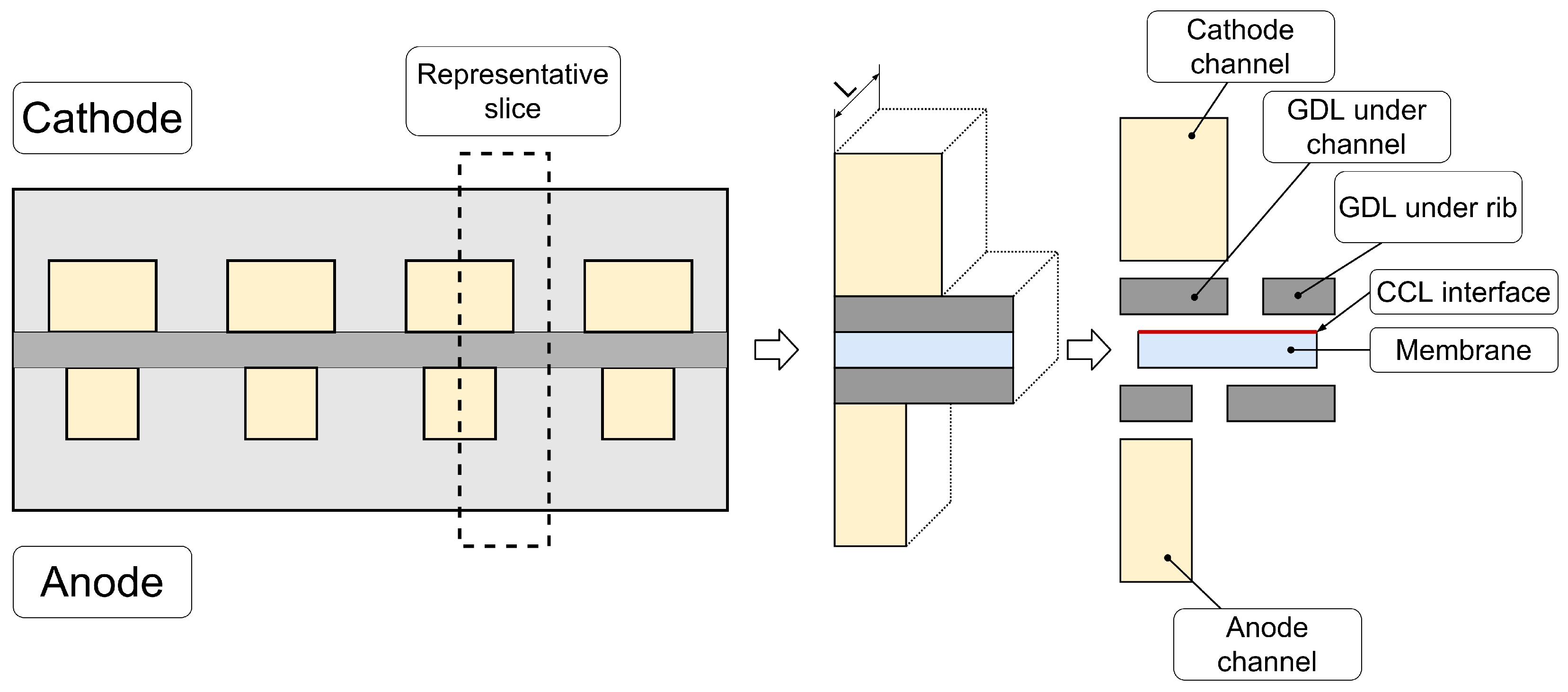
2.1. Numerical Model and Governing Equations

The transient, single-phase, isothermal, and hybrid analytical-numerical 3D model of a PEMFC implemented in AVL CRUISE™ M software was used for the simulations. The model, developed by Tavčar and Katrašnik [13], assumes the gas species in the channel flow direction (z-direction) to be 1D and solved numerically and the species concentrations perpendicular to the gas flow in the channel are calculated analytically in 2D ($x,y$-direction). The pressure drop in the GDL perpendicular to the gas flow in the channels is neglected. The model for the gas flow is coupled with an electrochemical sub-model. The electrode kinetics are reduced to the oxygen reduction reaction (ORR) of the cathode catalyst layer (CCL), which is assumed to be infinitesimally thin. The schematic overview of the modeled fuel cell is shown in Figure 1. A representative unit of assumed parallel channels and ribs is extracted. In the direction of the gas flow in the channel, this unit is discretized into an arbitrary number of slices with length L. The domains of the slice are as follows: cathode and anode channel, GDL parts under-channel, GDL parts under-rib, thin CCL and membrane. While the original model of Tavčar and Katrašnik [13] neglected the electrical conductivity of the GDL, the current implementation considers its ohmic losses. Liquid water is assumed to be present only inside the membrane. Its transport by water diffusion and electro-osmotic drag is assumed as being perpendicular to the membrane plane. Convection due to pressure differences between anode and cathode and a gas crossover through the membrane were not considered. The water content of the membrane is in equilibrium with the relative humidity of the gases mixture at the interface with the CL/GDL.

A more detailed view on the assumptions made during the development of the numerical model can be found in [13].

2.1.1. Governing Equations

The full set of equations of the hybrid 3D numerical model can be found in [13]. The following equations are highlighted because some of their parameters are used as design variables for the numerical optimization.

Species Transport in Gas Channels

The gas is assumed to be ideal and the species transport is modeled by Stefan–Maxwell diffusion. Only water vapor is modeled; liquid water is not considered in channels and GDLs, resulting in a single-phase approach. The species transport equation is divided into a 2D and a 1D part. In a channel slice it reads as follows [13]:

$$\frac{\mathrm{d}c}{\mathrm{d}t}=\underset{2\mathrm{D}}{\underbrace{{\nabla }^2(Dc-\tilde{c}V)}}-\underset{1\mathrm{D}}{\underbrace{{\partial }_z\left(vc\right)}}=0$$

(1)

With the concentration of species c in the channels and the velocity v in channel direction (z-direction). V represents the potential flow part of the gas flow in x- and y-direction. Due to steady-state assumption of the gas dynamics, the time derivative of the species concentration in Equation (1) is set to 0. The binary diffusion coefficient D and the average species concentration $\tilde{c}$ are constant in one slice. As there is no liquid phase, the relative humidity can reach values higher than 1. This was an indirect indication of liquid water formation.

Species Transport in GDLs

No gas flow (zero velocity) is assumed in z-direction in GDLs. Therefore, Equation (1) simplifies to

$$\frac{\mathrm{d}c(x,y)}{\mathrm{d}t}={\nabla }^2(D_{GDL}c(x,y)-\tilde{c}V(x,y))=0$$

(2)

where $D_{GDL}$ is the diffusion coefficient in the GDL. It is derived from the binary diffusion coefficient in gas channels by dividing D through the tortuosity ${\tau }_{GDL}$ of the GDL

$$D_{GDL}=\frac{D}{{\tau }_{GDL}}.$$

(3)

Electrochemical Reactions

The Butler–Volmer equation (BVE) is a relationship between the potential of an electrochemical system and its current density. The BVE states that the current density increases exponentially with activation overvoltage. In an electrochemical system such as a fuel cell, two independent BVEs for ACL and CCL can be employed. As the electrokinetics are reduced to the CCL by the model used, only the following BVE was applied [13,41]:

$$i=i_0\left(\frac{p_{O2}}{p_{ref}}{\mathrm{e}}^{\frac{\alpha nF}{RT}{\eta }_{act}}-{\left(\frac{p_{H2O}}{p_{ref}}\right)}^{\lambda }{\mathrm{e}}^{-\frac{(1-\alpha )nF}{RT}{\eta }_{act}}\right)$$

(4)

where $i_0$ represents the exchange current density, $p_{O2}$ and $p_{H2O}$ are partial pressures of oxygen and water, $\lambda$ stoichiometry ratio, $\alpha$ transfer coefficient, n number of exchanged electrons, F Faraday’s constant, T temperature and ${\eta }_{act}$ activation overpotential of the electrode. The exchange current density $i_0$ is related to the reference exchange current density $i_{0,ref}$ at reference temperature $T_{ref}$ and pressure $p_{ref}$ [13,41]

$$i_0=i_{0,ref}{\left(\frac{p_{O2}}{p_{ref}}\right)}^{b_{O2}}{\left(\frac{p_{H2O}}{p_{ref}}\right)}^{b_{O2}}{\mathrm{e}}^{\frac{E_{act,i_0}}{R}\left(\frac{1}{T_{ref}}-\frac{1}{T}\right)}$$

(5)

With $p_{O2}$ and $p_{H2O}$ partial pressures of oxygen and water, $b_{O2}$ and $b_{H2O}$ oxygen and water exponent and $E_{act,i_0}$ the activation energy of exchange current density.

Ionic Conductivity

The ionic conductivity of the membrane was calculated using the following Arrhenius approach with a reference ionic conductivity ${\sigma }_{ion,ref}$ at reference temperature $T_{ref}$ and reference membrane water content $C_{w,ref}$ [5]:

$${\sigma }_{ion}={\sigma }_{ion,ref}\frac{C_w}{C_{w,ref}}{\mathrm{e}}^{\frac{E_{act,{\sigma }_{ion}}}{R}\left(\frac{1}{T_{ref}}-\frac{1}{T_{mem}}\right)}$$

(6)

With $C_w$ actual water content of the membrane, $E_{act,{\sigma }_{ion}}$ activation energy, and $T_{mem}$ actual temperature of the membrane.

2.2. Numerical Optimization

Optimization algorithms search in general for the minimum of an objective function $f\left(\mathbf{x}\right)$ with one or more design variables $\mathbf{x}$ from the feasible design space $\mathcal{X}$. [42]

$$\begin{array}{c}\underset{\mathbf{x}}{\mathrm{minimize}}f\left(\mathbf{x}\right)\\ \\ \mathrm{subject}\mathrm{to}\mathbf{x}\in \mathcal{X}\end{array}$$

(7)

With $\mathbf{x}=[x_1,x_2,\dots ,x_n]$ for n-dimensional design variables. $\mathbf{x}$ can be varied to find the minimum of the objective function $f\left(\mathbf{x}\right)$.

There are two general optimization strategies, local optimization and global optimization. The local optimization aims to find the minimum near a starting point and the solution must not necessarily be a global minimum. In general, mathematical models of fuel cells are nonlinear, numerically stiff and non-differentiable. Therefore, optimization algorithms that rely on the derivative of the objective function are not applicable. Direct methods (e.g., Powell’s Method and Nelder–Mead Simplex Algorithm (NMSA)), stochastic methods (e.g., simulated annealing, natural evolution strategies) or population methods (e.g., genetic algorithms, differential-evolution, particle swarm optimization) are applied in case of non-differentiable objective functions. Whereas direct methods do not necessarily find the global minimum, stochastic and population methods search the given design space for the global optimum. Stochastic methods rely on pseudorandom strategies, such as Latin Hypercube Sampling (LHS) or Sobol sampling, to sample the design space and to escape local optima to enhance the probability of finding the global optimum. In contrast to direct and stochastic methods, population strategies do not move a single point toward the optimum, but use many design points (individuals) distributed throughout the design space. The information of the distributed design points is exchanged between the points to find the global minimum [42,43].

The scipy.optimization module from Python provides several local and global optimization algorithms. The differential evolution algorithm [43] gave the best and fastest results as a first indication of where to find the global minimum. The best combination of design variables from the differential-evolution optimizer was used as a starting point for a local optimizer, the Nelder–Mead Simplex Algorithm [44], to find the optimum more accurately.

As the simulations are transient, the objective value $Y_{Obj}$ is the integrated sum of the difference between the measured and the simulated voltage or current. As shown in Section 2.3, each of the three available measured polarization curves is based on six measured operating points. In the simulations, a current ramp from 0.02–1 $\mathrm{A}$/${\mathrm{cm}}^2$ with a total time of 720 $\mathrm{s}$ (which corresponds to a slope of $1.4$ $\mathrm{m}$$\mathrm{A}$/${\mathrm{cm}}^2$ per second) was defined. The difference of the simulated and measured voltage was then integrated over time to get the objective variable. For $U_{meas}\left(t\right)$ between the measured operating points, piecewise linear interpolation was applied.

$$Y_{Obj,PC}=\int \left|(U_{meas}\left(t\right)-U_{sim}\left(t\right))\right|\mathrm{d}t$$

(8)

The second set of available measured data were three load steps with voltage driven stacks, thus the difference between simulated and measured current was integrated.

$$Y_{Obj,LS}=\int \left|(I_{meas}\left(t\right)-I_{sim}\left(t\right))\right|\mathrm{d}t$$

(9)

All available measurements were used to optimize the parameters. Therefore, an appropriate combination of the objective value with weighting factors needed to be implemented. The results from the load steps were weighted with $2/3$, whereas the polarization curves were weighted with $1/3$. The three load steps and three polarization curves were weighted equally among themselves. The reason for shifting the weighting factor to the results of the load steps was that the focus was on the transient response of the FC and therefore, the main concern was to reproduce the measured load steps with as little error as possible.

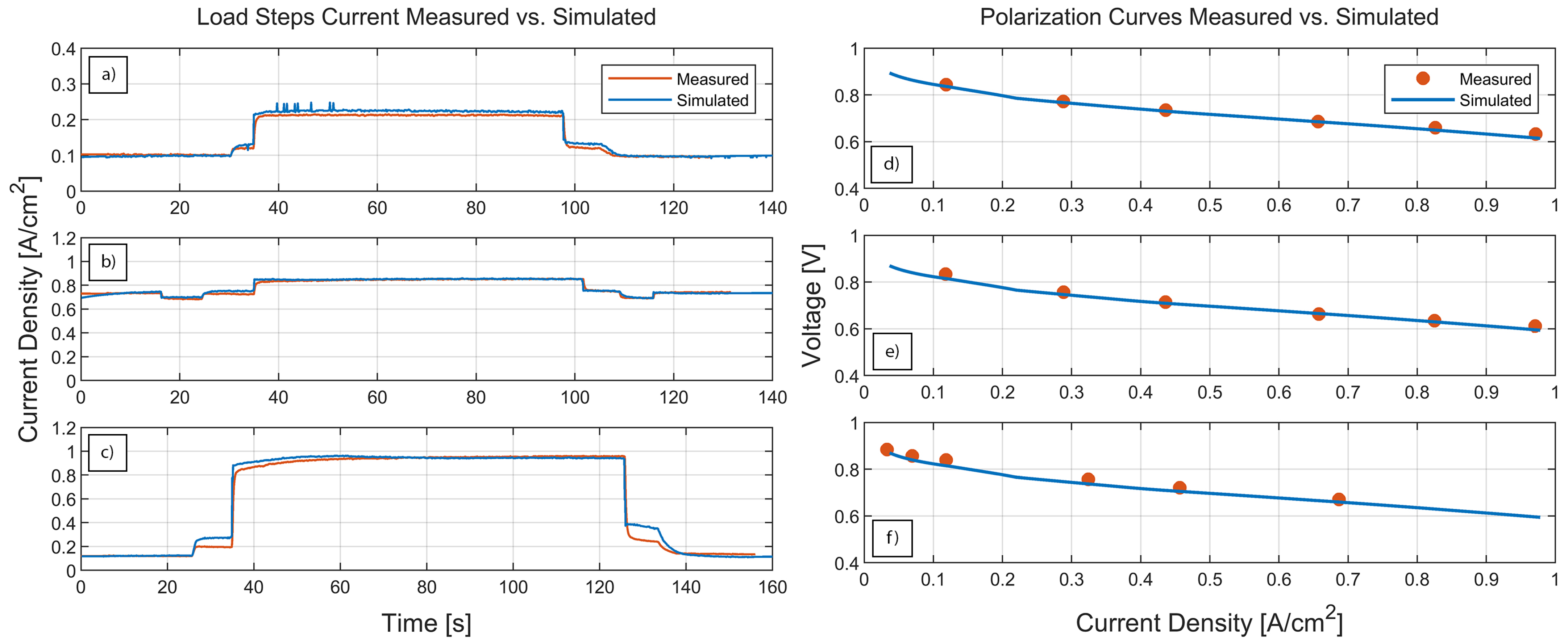
2.3. Experimental Results

The measurement data used in this work were obtained using a dedicated test stand equipped with a commercial 30 $\mathrm{k}$$\mathrm{W}$ fuel cell stack, the associated balance-of-plant components and a specifically designed measurement and control system. As the test stand has also been used for measurements in other publications and to avoid redundancy with other articles, the authors refer the reader to the work in [25,45] for a more detailed presentation of the test stand setup.

For the optimization of the parameters and validation of the simulation results, 6 measurement series were available, divided into three polarization curves and three load steps.

Table 1. Available measurement series from the test stand.

Name -	Type -	Anode Inlet Pressure mbar	Cooling Inlet Temperature ${}^{\circ }\mathbf{C}$
P1	Polarization Curve	1700	55
P2	Polarization Curve	1700	52
P3	Polarization Curve	1400	55
L1	Load Step	1700	55
L2	Load Step	1700	55
L3	Load Step	1700	55

gives an overview of the measured data series.

For all measurements, the stoichiometry at the cathode was ${\lambda }_{cat}=2$ for current densities below $0.12$ $\mathrm{A}$/${\mathrm{cm}}^2$ and ${\lambda }_{cat}=1.5$ for current densities exceeding $0.22$ $\mathrm{A}$/${\mathrm{cm}}^2$. Anode stoichiometry was a product of mixing the recirculated humid hydrogen with dry hydrogen from the hydrogen storage system. The rotational speed of the hydrogen recirculation pump (HRP) was set to a constant value, hence the anode stoichiometry was not constant. It ranged from approx. 6 at low currents to 1.6 at high currents. The anode inlet relative humidity was set to 99% and the pressure was set to a constant value ( 1700 $\mathrm{mbar}$ or 1400 $\mathrm{mbar}$). Ambient air conditions during the measurements can be found in

Table 2. Ambient air conditions during measurements at the test stand.

Parameter	Unit	Value
Temperature	${}^{\circ }\mathrm{C}$	23
Pressure	mbar	983
Relative Humidity	%	48

.

A constant air inlet temperature of 40 ${}^{\circ }\mathrm{C}$ could be achieved due to an air cooler downstream of the compressor. The polarization curves were recorded by current controlled stack at different cooling inlet temperatures and anode inlet pressures, as shown in Table 1.

For each of the measured polarization curves six measured points in the current range of 0.1–1 $\mathrm{A}$/${\mathrm{cm}}^2$ were available, as shown in Figure 2. The series of measurements with the load steps were recorded by voltage-controlled stack. Three different load steps were available:

• L1 is recorded with cell potential from 844 $\mathrm{m}$$\mathrm{V}$ to 792 $\mathrm{m}$$\mathrm{V}$ to 844 $\mathrm{m}$$\mathrm{V}$
• L2 is recorded with cell potential from 666 $\mathrm{m}$$\mathrm{V}$ to 640 $\mathrm{m}$$\mathrm{V}$ to 666 $\mathrm{m}$$\mathrm{V}$
• L3 is recorded with cell potential from 834 $\mathrm{m}$$\mathrm{V}$ to 630 $\mathrm{m}$$\mathrm{V}$ to 834 $\mathrm{m}$$\mathrm{V}$

Which corresponds to approximately $0.12$ $\mathrm{A}$/${\mathrm{cm}}^2$ to $0.22$ $\mathrm{A}$/${\mathrm{cm}}^2$ to $0.12$ $\mathrm{A}$/${\mathrm{cm}}^2$ for L1, $0.73$ $\mathrm{A}$/${\mathrm{cm}}^2$ to $0.85$ $\mathrm{A}$/${\mathrm{cm}}^2$ to $0.73$ $\mathrm{A}$/${\mathrm{cm}}^2$ for L2 and $0.12$ $\mathrm{A}$/${\mathrm{cm}}^2$ to $0.95$ $\mathrm{A}$/${\mathrm{cm}}^2$ to $0.12$ $\mathrm{A}$/${\mathrm{cm}}^2$ for L3. Figure 3 shows the measured cell potential and cell current over time.

3. Results

3.1. Hybrid 3D Model Details

The analyzed commercial PEMFC consisted of bipolar plates made of fuel cell grade graphite, carbon paper GDLs with hydrophobic PTFE coating, and an ultra-thin automotive-grade PEM made from SSC-PFSA with reinforcement. The thicknesses of the fuel cell components are listed in

Table 3. Dimensions of fuel cell components. Thicknesses for GDL (at 1 $\mathrm{M}$$\mathrm{Pa}$ compression) and membrane were taken from manufacturers datasheet.

		Cathode			Anode		Membrane
Parameter	Unit	BPP	GDL	CL	BPP	GDL
Thickness	$\mathrm{m}\mathrm{m}$	1.65	0.21	0.01	1.65	0.21	0.015
Channel width	$\mathrm{m}\mathrm{m}$	1.1			0.6
Channel height	$\mathrm{m}\mathrm{m}$	0.5			0.5

.

The model consisted of three different circuits: (1) gas circuit, (2) electrical circuit, and (3) thermal circuit to set the operating temperature. In the direction of the gas flow in the channel, the fuel cell was divided into six slices, which was a compromise between accuracy and computation time. Species mass flows, pressures, and temperatures were applied as described in Section 2.3.

Parameterization

Numerical optimization algorithms were used to find the best values for a selected set of parameters. The following parameters were design variables for the optimization process (1) RECD, (2) activation energy of exchange current density of the CCL, (3) transfer coefficient of the CCL, (4) reference membrane ionic conductivity, (5) activation energy of the ionic conductivity, (6) electrical conductivity, (7) porosity, and (8) tortuosity of the GDL.

Table 4. Assumed material parameters of the investigated fuel cell. Effective values are shown for material properties of GDL. Parameters marked with ⧫ are design variables for numerical optimization.

Parameter		Unit	BPP	GDL	CCL	Membrane
Density		$\mathrm{k}\mathrm{g}/{\mathrm{m}}^3$	1900	2000		1980
Electrical Conductivity		$\mathrm{S}/\mathrm{m}$	2000	⧫
Porosity		-		⧫
Tortuosity		-		⧫
Ionic Conductivity
	${\sigma }_{ion,ref}$	$\mathrm{S}/\mathrm{m}$				⧫
	$C_{W,ref}$	-				14
	Reference Temperature	${}^{\circ }\mathrm{C}$				55
	Activation Energy	$\mathrm{J}/\mathrm{mol}$				⧫
Water Diffusion Coefficient
	$D_{W,ref}$	${\mathrm{m}}^2/\mathrm{s}$				2.16 × 10−11
	$C_{W,ref,D_W}$	-				1
	Reference Temperature	${}^{\circ }\mathrm{C}$				25
	Activation Energy	$\mathrm{J}/\mathrm{mol}$				19,809
Electro-osmotic Drag Coef.
	$n_{drag,ref}$	-				0.1136
	$C_{W,ref,n_{drag}}$	-				1
Equilibrium Water Content		-				Springer
Transfer Coefficient		-			⧫
Exchange Current Density
	RECD	$\mathrm{A}/{\mathrm{cm}}^2$			⧫
	Reference Temperature	${}^{\circ }\mathrm{C}$			55
	Activation Energy	$\mathrm{J}/\mathrm{mol}$			⧫
Water Exponent		-			1
Oxygen Exponent		-			0.75

gives an overview of the used material parameters and the design variables are marked with ⧫. As the electrochemical parameters of the CCL are mostly unknown, a common practice is to use these parameters for calibration of the electrochemical model, see, e.g., in [18,46,47,48]. As the temperature influence of the RECD was unknown, the activation energy of the Arrhenius term (see Equation (5)) was selected as a design variable. Although the ionic conductivity could be found in datasheets of the membrane in H-form and for fully hydrated membrane at a reference temperature, the temperature dependence was not available for the given membrane material. Therefore, the activation energy of the temperature dependence and the ionic conductivity were added to the design variables for the optimization process. Due to the lack of information on the water sorption behavior of the used membrane, the model suggested by Springer [5] was applied. The water diffusion coefficient and electro-osmotic drag coefficient were taken from standard ionomer material. For the fluid flow through porous media, the porosity is crucial. As shown by Karpenko-Jereb et al. [22] and d’Adamo et al. [19] the porosity of the GDLs has a significant influence on the species transport, electric conductivity and, therefore, current density. Thus, the porosity was added to the design variables for numerical optimization. Although the tortuosity of the GDLs can be estimated with the porosity as proposed by [49] (Other relationships in the literature can be found in [49,50,51].), it was used as a design variable as well.

3.2. Optimization

The results of the optimization process and the comparison between the measured values from the test stand with the simulated results are described in this section. The numerical optimization with the differential-evolution algorithm was started with the bounds shown in

Table 5. Bounds of the design variables for global optimization and results from the numerical optimization process. DiffEvo represents the values obtained from the differential-evolution algorithm. These parameters are used as starting vector for the Nelder–Mead Simplex Algorithm to find the local minimum more accurately. The final set of parameters is shown in row NelderMead.

Parameter	${\mathit{i}}_{0,\mathit{ref}}$	${\mathit{E}}_{\mathit{act},{\mathit{i}}_0,\mathit{ref}}$	$\mathit{\alpha }$	${\mathit{\sigma }}_{\mathit{ion},\mathit{ref}}$	${\mathit{E}}_{\mathit{act},\mathit{\sigma },\mathit{ion}}$	${\mathit{\sigma }}_{\mathit{elec},\mathit{GDL}}$	${\mathit{\epsilon }}_{\mathit{GDL}}$	${\mathit{\tau }}_{\mathit{GDL}}$
Unit	A/cm2	J/mol	-	S/m	J/mol	S/m	-	-
Bound min	2.00 × 10 −4	50,000	0.3	4	10,000	80	0.4	1
Bound max	2.00 × 10 −3	250,000	0.4	20	50,000	390	0.8	3
DiffEvo	4.884 × 10 −4	226,071	0.333	14.97	66,037	356.6	0.63	1.16
NelderMead	6.732 × 10 −4	213,475	0.32	14.03	35,486	355.8	0.69	1.00

. The differential-evolution strategy was set to ’best1bin’. This strategy chooses two members randomly and their difference is used for the mutation of the best member to construct a trial vector. For more information, see in [40,52]. The initial sampling of the design space was done with the Latin hypercube sequence to maximize the coverage of the available parameter space. The recombination constant (crossover probability) was left to the default number of $0.7$. The relative tolerance for convergence was set to $0.01$. The global optimization with the differential-evolution algorithm was stopped after 72 $\mathrm{h}$ or 1412 function evaluations to limit the computation time. One simulation of a design point takes around 170 $\mathrm{s}$ for all six cases. The design point with the lowest integrated difference between simulated and measured value, see Equation (9), was calculated at iteration 957. The set of parameters from the differential-evolution algorithm was used as a starting point for the NMSA to perform a local optimization. The absolute tolerance and function tolerance of the Nelder–Mead Algorithm were set to $0.01$. This condition was met after 745 model evaluations. Figure 4 shows the course of the objective value over the iterations of the model. Not every parameter combination leads to a good result. If the simulation time exceeds a certain value, the design point is not feasible and the objective value is set to an artificially high value (1000) not to influence the optimization result. In Figure 4 these values are not shown.

The bounds specified in Table 5 were used by the differential-evolution algorithm for the sampling of the design space, whereas the implemented NMSA searched for the minimum without bounds. Therefore, it would be possible to get parameters outside of the specified bounds with the NMSA. The final design variables with the lowest integrated difference are shown in Table 5.

The values obtained from numerical optimization for the design variables agree well with the standard physical values found in the literature, as shown below.

3.2.1. Activation Energies

As in the introduction already mentioned, the measurements showed strong temperature dependence, therefore the activation energies of the Arrhenius terms in the exchange current density ($E_{act,i_0,ref}$) and the ionic conductivity ($E_{act,\sigma ,ion}$) showed higher values than in the literature found. For the activation energy of the exchange current density, a common value is $E_{act,i_0,ref}=66\times {10}^3\mathrm{J}/\mathrm{mol}$ [22,48] and for the activation energy of the ionic conductivity near $E_{act,\sigma ,ion}=10\times {10}^3\mathrm{J}/\mathrm{mol}$, e.g., $E_{act,\sigma ,ion}=10,542\mathrm{J}/\mathrm{mol}$ [5] or $E_{act,\sigma ,ion}=9894\mathrm{J}/\mathrm{mol}$ [53] for Nafion^® N117.

3.2.2. Reference Exchange Current Density and Transfer Coefficient

The exact values for the RECD and transfer coefficient of the CCL were not known. Therefore, these variables were used for the calibration of the model. The value presented, e.g., in [54] with $9\times {10}^{-9}$ $\mathrm{A}$/${\mathrm{m}}_2^{\mathrm{Pt}}$, for the ORR with Pt-C is specified per unit area of metal, while the model used in this work relates the RECD to the active area of the fuel cell. Since the real surface area of the platinum for the CCL is unknown, the value obtained from the optimization process cannot be directly compared with values from the literature. The optimized transfer coefficient with $\alpha =0.33$ lies within the bounds for oxygen reduction reactions (ORR) of hydrogen fuel cells ($0.1$ to $0.5$) as shown in [55].

Ionic Conductivity

The ionic conductivity of the membrane can be found in the datasheet provided by the manufacturer with 14 $\mathrm{S}$/$\mathrm{m}$ for fully hydrated membrane at a temperature of 25 ${}^{\circ }\mathrm{C}$. The obtained value from the optimization process is with 14 $\mathrm{S}$/$\mathrm{m}$ at $T_{ref}=55{}^{\circ }\mathrm{C}$ lower for the higher reference temperature (The higher the temperature, the higher the ionic conductivity). The reasons for this difference can be that there is an uncertainty if the values from the datasheet were obtained with a fully hydrated membrane activated with 10% H₂SO₄ at 80 ${}^{\circ }\mathrm{C}$ or the reference water concentration $C_{w,ref}=14$ is not the highest possible water concentration of the used membrane. As the water sorption isotherm was not known and the relationship from Springer [5] was used for the simulations, the uncertainty may be in the use of this relationship. However, the obtained value is within physical bounds for SSC-PFSA ionomers [56,57,58].

3.2.3. GDL Electrical Conductivity

The effective electrical conductivity of the GDL ${\sigma }_{elec,gdl}=355.8\mathrm{S}/\mathrm{m}$ is higher than given by the datasheet of the manufacturer with $262.5$ $\mathrm{S}$/$\mathrm{m}$ at 1 $\mathrm{M}$$\mathrm{Pa}$ compression. The exact value of the stacked cells’ compression is unknown, so this could be a reason for the higher value. Another factor is the calculation of the effective value of porous media. The effective electrical conductivity is a function of the bulk electrical conductivity and the porosity of the GDL. Several different relationships can be found in the literature, see in [19]. As proposed by Bruggeman [50] and adapted by Das et al. [59] the relationship of effective and bulk conductivity can be given with

$${\sigma }_{eff}={\sigma }_{bulk}·{(1-\epsilon )}^{1.5}$$

(10)

With ${\sigma }_{bulk}$ the bulk conductivity of the solid and $\epsilon$ the porosity of the material. However, the software used has implemented the following relationship for the effective conductivity:

$${\sigma }_{eff}={\sigma }_{bulk}·(1-\epsilon )$$

(11)

The effective value was specified during the optimization process and the software calculated the bulk electrical conductivity with the above relationship. The bulk electrical conductivity and the solid fraction of the porous media were then used to determine the ohmic losses of the GDLs. The electrical conductivity of commercially available carbon paper GDLs with hydrophobic treatment ranges from 150–350 $\mathrm{S}$/$\mathrm{m}$ (effective value in an uncompressed state); thus, the obtained value is comparable.

3.2.4. GDL Porosity and Tortuosity

The porosity with ${\epsilon }_{GDL}=0.69$ and the tortuosity ${\tau }_{GDL}=1.0$ obtained from the numerical optimization agree with common values for GDLs in the literature. In addition, the porosity can be estimated with the area weight given by the datasheet from the manufacturer and an estimated compression of approx. 1 $\mathrm{M}$$\mathrm{Pa}$ with ${\epsilon }_{GDL,est}=0.7$. This value is close to the result of the numerical optimization procedure. The tortuosity of the GDL is mostly unknown, thus several relationships exist in the literature to determine it from the porosity of the material, see in [19]. A value of about ${\tau }_{GDL,expected}=1.38$ could be expected from the optimization process by applying the schemes on the determined porosity. However, the obtained value of ${\tau }_{GDL}=1.0$ is low. The diffusion length of the GDL and the thickness are not the same in reality. Moreover, ${\tau }_{GDL}=1.0$ is equivalent to free diffusion of gas species through the GDL as the binary and actual diffusion coefficients, see Equation (3) have the same value.

With the parameter set from the numerical optimization the following results can be obtained.

The simulations showed very good agreement with the measurements, as can be seen in Figure 5. Although the weighting factors favored the load levels, the results of the simulated polarization curves differed only slightly from the measured data with average relative errors of $\Delta P1=1.01\%$, $\Delta P2=1.35\%$, and $\Delta P3=0.54\%$. The load step in the high current region, L2, agreed very well, whereas L1 in the low current region showed more deviation to the comparison data. However, the load step over the entire current range, L3, agreed well with the measurements. In addition, the current after the load step was represented well by the model. The small current steps before and after the main load steps came from the measurement from the test stand and were necessary to ensure the stable operation of the stack.

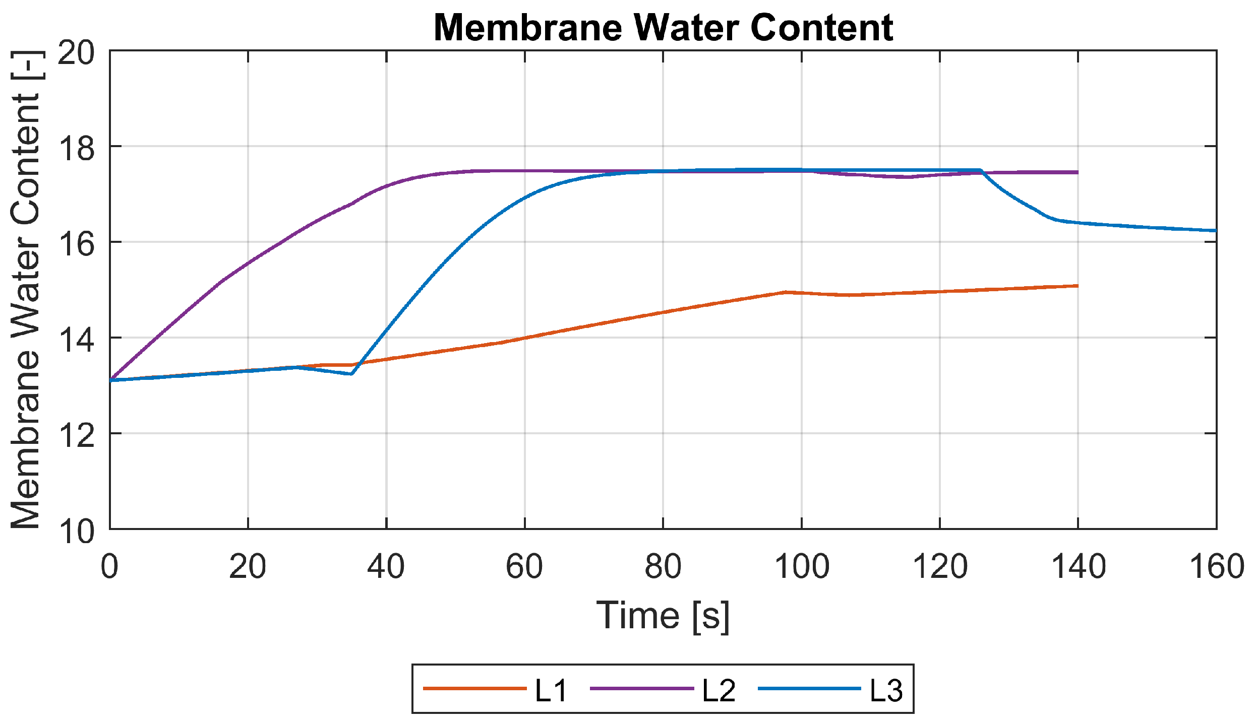
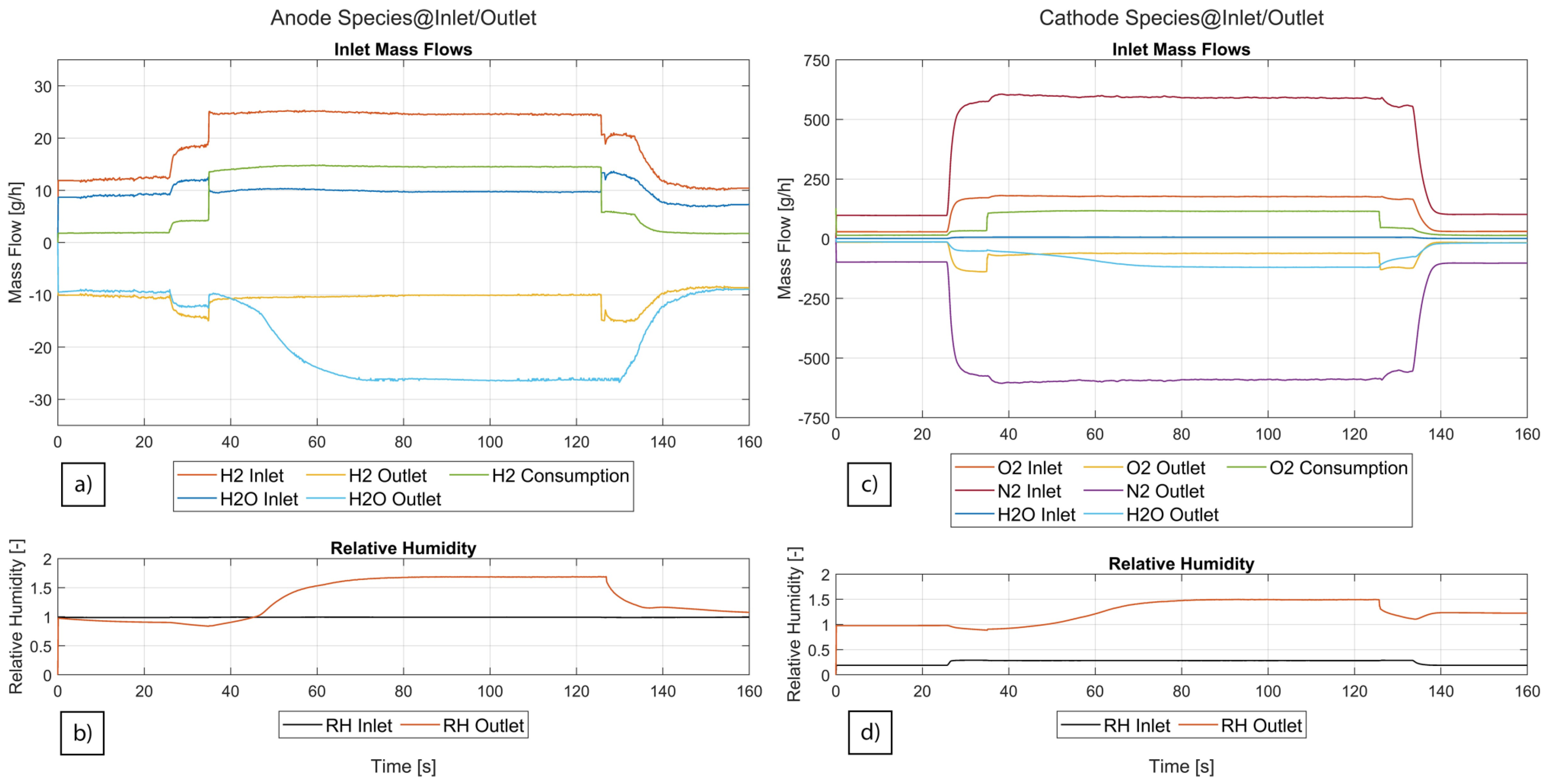
3.3. Species Mass Flows and Membrane Water Content

H₂ and H₂O-vapor mass flows at anode in- and outlet as well as O₂, N₂ and H₂O-vapor mass flows at cathode in- and outlet for load step L3 are shown in Figure 6. Negative values indicate mass flows at outlets. It can be observed that the water vapor mass flow at the anode outlet in Figure 6a increased after the load step and the operation of the fuel cell at $0.95$ $\mathrm{A}$/${\mathrm{cm}}^2$. The relative humidity also increased and remained at a constant value until the current dropped back to $0.12$ $\mathrm{A}$/${\mathrm{cm}}^2$. The relative humidity at the cathode outlet approached a maximum value of 1.5 after the load step to $0.95$ $\mathrm{A}$/${\mathrm{cm}}^2$. The water vapor mass flows at the anode and the cathode outlet increased steadily. Due to water diffusion through the membrane, the water vapor concentration at the anode also increased.

Figure 7 shows the membrane water content $C_w$ for all three load steps over time. $C_w$ for load step L1 is lower than for L2 and L3. The current densities L2 and L3 after the load step were much higher than for L1. Therefore more water was produced by the chemical reaction in the CCL. This water increased the relative humidity in the cathode and was sorbed by the membrane. The maximum membrane water content was given with 17.5.

4. Conclusions

The parameterization of mechanistic models for PEMFCs is challenging. Developing more sophisticated models with, e.g., anisotropic material properties, agglomerate models for CL or gas crossover in the membrane further exacerbates the problem. The measurement methods to determine the necessary parameters are complex, expensive, and specialized equipment is often needed, e.g., the porosity of the GDL can be measured via 3D XCT methods, see [19]. This work demonstrated the efficient parameterization of a single-phase, isothermal PEMFC model with measurements on a stack. The measurements showed a strong temperature dependence and the operating temperature is relatively low with 52–55 ${}^{\circ }\mathrm{C}$ (cooling inlet). Therefore, special attention was paid to the activation energies of the Arrhenius terms of the RECD and the ionic conductivity of the membrane.

The following parameters were selected as design variables for numerical optimization: (1) RECD of CCL, (2) activation energy of the exchange current density, (3) transfer coefficient of the CCL, (4) reference membrane ionic conductivity, (5) activation energy of the ionic conductivity, (6) electrical conductivity, (7) porosity, and (8) tortuosity of the GDL. The numerical optimization was conducted with the Python package scipy.optimize. The differential-evolution algorithm for global optimization and the Nelder–Mead algorithm for local optimization were used. It was shown that both algorithms were well suited for this type of engineering problem and fast convergence of the objective value was given. With these optimized parameters, the simulated and measured polarization curves and load steps agreed very well. Although numerical optimization had found good values for the selected design variables, it does not necessarily replace advanced measurement methods to determine the unknown parameters in advance. Further activities will be necessary here in the future.

However, the measurement of the load steps and polarization curves in conjunction with the in- and outlet mass flows, pressures, humidities and temperatures, and cooling temperatures were sufficient to parameterize the fuel cell model used. Due to the lack of measured material data, the optimized parameters were compared with values from the literature. They agreed well with the typical physical values of the eight design variables, although the exact values remain unknown. The obtained material parameters will be used in the future to parameterize a more detailed 3D CFD model to analyze the transient behavior of PEMFCs at low operating temperatures with high spatial and temporal resolution.

References

1. Bethoux, O. Hydrogen Fuel Cell Road Vehicles: State of the Art and Perspectives. Energies 2020, 13, 5843. [Google Scholar] [CrossRef]
2. Ritzberger, D.; Hametner, C.; Jakubek, S. A Real-Time Dynamic Fuel Cell System Simulation for Model-Based Diagnostics and Control: Validation on Real Driving Data. Energies 2020, 13, 3148. [Google Scholar] [CrossRef]
3. Cheddie, D.; Munroe, N. Review and comparison of approaches to proton exchange membrane fuel cell modeling. J. Power Sources 2005, 147, 72–84. [Google Scholar] [CrossRef]
4. Demuren, A.; Edwards, R.L. Modeling Proton Exchange Membrane Fuel Cells—A Review. In 50 Years of CFD in Engineering Sciences; Runchal, A., Ed.; Springer: Singapore, 2020; pp. 513–547. [Google Scholar] [CrossRef]
5. Springer, T.E. Polymer Electrolyte Fuel Cell Model. J. Electrochem. Soc. 1991, 138, 2334. [Google Scholar] [CrossRef]
6. Bernardi, D.M.; Verbrugge, M.W. A Mathematical Model of the Solid-Polymer-Electrolyte Fuel Cell. J. Electrochem. Soc. 1992, 139, 2477. [Google Scholar] [CrossRef]
7. Maggio, G.; Recupero, V.; Pino, L. Modeling polymer electrolyte fuel cells: An innovative approach. J. Power Sources 2001, 101, 275–286. [Google Scholar] [CrossRef]
8. Wohr, M. Dynamic modelling and simulation of a polymer membrane fuel cell including mass transport limitation. Int. J. Hydrogen Energy 1998, 23, 213–218. [Google Scholar] [CrossRef]
9. Gao, F.; Blunier, B.; Miraoui, A.; El Moudni, A. A Multiphysic Dynamic 1-D Model of a Proton-Exchange-Membrane Fuel-Cell Stack for Real-Time Simulation. IEEE Trans. Ind. Electron. 2010, 57, 1853–1864. [Google Scholar] [CrossRef]
10. Murschenhofer, D.; Kuzdas, D.; Braun, S.; Jakubek, S. A real-time capable quasi-2D proton exchange membrane fuel cell model. Energy Convers. Manag. 2018, 162, 159–175. [Google Scholar] [CrossRef]
11. Futter, G.A.; Gazdzicki, P.; Friedrich, K.A.; Latz, A.; Jahnke, T. Physical modeling of polymer-electrolyte membrane fuel cells: Understanding water management and impedance spectra. J. Power Sources 2018, 391, 148–161. [Google Scholar] [CrossRef]
12. Goshtasbi, A.; Pence, B.L.; Chen, J.; DeBolt, M.A.; Wang, C.; Waldecker, J.R.; Hirano, S.; Ersal, T. A Mathematical Model toward Real-Time Monitoring of Automotive PEM Fuel Cells. J. Electrochem. Soc. 2020, 167, 024518. [Google Scholar] [CrossRef]
13. Tavčar, G.; Katrašnik, T. An Innovative Hybrid 3D Analytic-Numerical Approach for System Level Modelling of PEM Fuel Cells. Energies 2013, 6, 5426–5485. [Google Scholar] [CrossRef] [Green Version]
14. Tavčar, G.; Katrašnik, T. A computationally efficient hybrid 3D analytic-numerical approach for modelling species transport in a proton exchange membrane fuel cell. J. Power Sources 2013, 236, 321–340. [Google Scholar] [CrossRef]
15. Pant, L.M.; Gerhardt, M.R.; Macauley, N.; Mukundan, R.; Borup, R.L.; Weber, A.Z. Along-the-channel modeling and analysis of PEFCs at low stoichiometry: Development of a 1+2D model. Electrochim. Acta 2019, 326, 134963. [Google Scholar] [CrossRef] [Green Version]
16. Berning, T.; Djilali, N. A 3D, Multiphase, Multicomponent Model of the Cathode and Anode of a PEM Fuel Cell. J. Electrochem. Soc. 2003, 150, A1589. [Google Scholar] [CrossRef]
17. Wu, H.; Berg, P.; Li, X. Steady and unsteady 3D non-isothermal modeling of PEM fuel cells with the effect of non-equilibrium phase transfer. Appl. Energy 2010, 87, 2778–2784. [Google Scholar] [CrossRef]
18. Fink, C.; Fouquet, N. Three-dimensional simulation of polymer electrolyte membrane fuel cells with experimental validation. Electrochim. Acta 2011, 56, 10820–10831. [Google Scholar] [CrossRef]
19. d’Adamo, A.; Haslinger, M.; Corda, G.; Höflinger, J.; Fontanesi, S.; Lauer, T. Modelling Methods and Validation Techniques for CFD Simulations of PEM Fuel Cells. Processes 2021, 9, 688. [Google Scholar] [CrossRef]
20. Dickinson, E.J.F.; Smith, G. Modelling the Proton-Conductive Membrane in Practical Polymer Electrolyte Membrane Fuel Cell (PEMFC) Simulation: A Review. Membranes 2020, 10, 310. [Google Scholar] [CrossRef]
21. Vetter, R.; Schumacher, J.O. Experimental parameter uncertainty in proton exchange membrane fuel cell modeling. Part I: Scatter in material parameterization. J. Power Sources 2019, 438, 227018. [Google Scholar] [CrossRef] [Green Version]
22. Karpenko-Jereb, L.; Sternig, C.; Fink, C.; Hacker, V.; Theiler, A.; Tatschl, R. Theoretical study of the influence of material parameters on the performance of a polymer electrolyte fuel cell. J. Power Sources 2015, 297, 329–343. [Google Scholar] [CrossRef]
23. Vetter, R.; Schumacher, J.O. Experimental parameter uncertainty in proton exchange membrane fuel cell modeling. Part II: Sensitivity analysis and importance ranking. J. Power Sources 2019, 439, 126529. [Google Scholar] [CrossRef] [Green Version]
24. Laoun, B.; Naceur, M.W.; Khellaf, A.; Kannan, A.M. Global sensitivity analysis of proton exchange membrane fuel cell model. Int. J. Hydrogen Energy 2016, 41, 9521–9528. [Google Scholar] [CrossRef]
25. Du, Z.P.; Steindl, C.; Jakubek, S. Efficient Two-Step Parametrization of a Control-Oriented Zero-Dimensional Polymer Electrolyte Membrane Fuel Cell Model Based on Measured Stack Data. Processes 2021, 9, 713. [Google Scholar] [CrossRef]
26. Kravos, A.; Ritzberger, D.; Hametner, C.; Jakubek, S.; Katrašnik, T. Methodology for efficient parametrisation of electrochemical PEMFC model for virtual observers: Model based optimal design of experiments supported by parameter sensitivity analysis. Int. J. Hydrogen Energy 2021, 46, 13832–13844. [Google Scholar] [CrossRef]
27. Ritzberger, D.; Höflinger, J.; Du, Z.P.; Hametner, C.; Jakubek, S. Data-driven parameterization of polymer electrolyte membrane fuel cell models via simultaneous local linear structured state space identification. Int. J. Hydrogen Energy 2021, 46, 11878–11893. [Google Scholar] [CrossRef]
28. Goshtasbi, A.; Chen, J.; Waldecker, J.R.; Hirano, S.; Ersal, T. Effective Parameterization of PEM Fuel Cell Models—Part II: Robust Parameter Subset Selection, Robust Optimal Experimental Design, and Multi-Step Parameter Identification Algorithm. J. Electrochem. Soc. 2020, 167, 044505. [Google Scholar] [CrossRef]
29. Goshtasbi, A.; Chen, J.; Waldecker, J.R.; Hirano, S.; Ersal, T. Effective Parameterization of PEM Fuel Cell Models—Part I: Sensitivity Analysis and Parameter Identifiability. J. Electrochem. Soc. 2020, 167, 044504. [Google Scholar] [CrossRef]
30. Abaza, A.; El-Sehiemy, R.A.; Mahmoud, K.; Lehtonen, M.; Darwish, M.M.F. Optimal Estimation of Proton Exchange Membrane Fuel Cells Parameter Based on Coyote Optimization Algorithm. Appl. Sci. 2021, 11, 2052. [Google Scholar] [CrossRef]
31. Sedighizadeh, M.; Rezazadeh, A.; Khoddam, M.; Zarean, N. Parameter Optimization for a Pemfc Model With Particle Swarm Optimization. Int. J. Eng. Appl. Sci. 2011, 3, 102–108. [Google Scholar]
32. El-Fergany, A.A. Extracting optimal parameters of PEM fuel cells using Salp Swarm Optimizer. Renew. Energy 2018, 119, 641–648. [Google Scholar] [CrossRef]
33. Salim, R.; Nabag, M.; Noura, H.; Fardoun, A. The parameter identification of the Nexa 1.2 kW PEMFC’s model using particle swarm optimization. Renew. Energy 2015, 82, 26–34. [Google Scholar] [CrossRef]
34. Yuan, Z.; Wang, W.; Wang, H.; Ashourian, M. Parameter identification of PEMFC based on Convolutional neural network optimized by balanced deer hunting optimization algorithm. Energy Rep. 2020, 6, 1572–1580. [Google Scholar] [CrossRef]
35. Fathy, A.; Rezk, H. Multi-verse optimizer for identifying the optimal parameters of PEMFC model. Energy 2018, 143, 634–644. [Google Scholar] [CrossRef]
36. Mo, Z.J.; Zhu, X.J.; Wei, L.Y.; Cao, G.Y. Parameter optimization for a PEMFC model with a hybrid genetic algorithm. Int. J. Energy Res. 2006, 30, 585–597. [Google Scholar] [CrossRef]
37. Sun, Z.; Wang, N.; Bi, Y.; Srinivasan, D. Parameter identification of PEMFC model based on hybrid adaptive differential evolution algorithm. Energy 2015, 90, 1334–1341. [Google Scholar] [CrossRef]
38. Gong, W.; Yan, X.; Liu, X.; Cai, Z. Parameter extraction of different fuel cell models with transferred adaptive differential evolution. Energy 2015, 86, 139–151. [Google Scholar] [CrossRef]
39. Sun, Z.; Cao, D.; Ling, Y.; Xiang, F.; Sun, Z.; Wu, F. Proton exchange membrane fuel cell model parameter identification based on dynamic differential evolution with collective guidance factor algorithm. Energy 2021, 216, 119056. [Google Scholar] [CrossRef]
40. Virtanen, P.; Gommers, R.; Oliphant, T.E.; Haberland, M.; Reddy, T.; Cournapeau, D.; Burovski, E.; Peterson, P.; Weckesser, W.; Bright, J.; et al. SciPy 1.0: Fundamental Algorithms for Scientific Computing in Python. Nat. Methods 2020, 17, 261–272. [Google Scholar] [CrossRef] [PubMed] [Green Version]
41. Barbir, F. PEM Fuel Cells: Theory and Practice, 2nd ed.; Elsevier: Amsterdam, The Netherlands; Academic Press: Boston, MA, USA, 2013. [Google Scholar]
42. Kochenderfer, M.J.; Wheeler, T.A. Algorithms for Optimization; The MIT Press: Cambridge, MA, USA; London, UK, 2019. [Google Scholar]
43. Storn, R.; Price, K. Differential Evolution—A Simple and Efficient Heuristic for Global Optimization over Continuous Spaces. J. Glob. Optim. 1997, 11, 341–359. [Google Scholar] [CrossRef]
44. Gao, F.; Han, L. Implementing the Nelder-Mead simplex algorithm with adaptive parameters. Comput. Optim. Appl. 2012, 51, 259–277. [Google Scholar] [CrossRef]
45. Hoeflinger, J.; Hofmann, P.; Geringer, B. Experimental PEM-Fuel Cell Range Extender System Operation and Parameter Influence Analysis; SAE Technical Paper Series; SAE International400 Commonwealth Drive: Warrendale, PA, USA, 2019. [Google Scholar] [CrossRef]
46. Karpenko-Jereb, L.; Innerwinkler, P.; Kelterer, A.M.; Sternig, C.; Fink, C.; Prenninger, P.; Tatschl, R. A novel membrane transport model for polymer electrolyte fuel cell simulations. Int. J. Hydrogen Energy 2014, 39, 7077–7088. [Google Scholar] [CrossRef]
47. Bednarek, T.; Tsotridis, G. Issues associated with modelling of proton exchange membrane fuel cell by computational fluid dynamics. J. Power Sources 2017, 343, 550–563. [Google Scholar] [CrossRef]
48. Fink, C.; Karpenko-Jereb, L.; Ashton, S. Advanced CFD Analysis of an Air-cooled PEM Fuel Cell Stack Predicting the Loss of Performance with Time. Fuel Cells 2016, 16, 490–503. [Google Scholar] [CrossRef] [Green Version]
49. Tomadakis, M.M.; Robertson, T.J. Viscous Permeability of Random Fiber Structures: Comparison of Electrical and Diffusional Estimates with Experimental and Analytical Results. J. Compos. Mater. 2005, 39, 163–188. [Google Scholar] [CrossRef]
50. Bruggeman, D.A.G. Berechnung verschiedener physikalischer Konstanten von heterogenen Substanzen. I. Dielektrizitätskonstanten und Leitfähigkeiten der Mischkörper aus isotropen Substanzen. Ann. Phys. 1935, 416, 636–664. [Google Scholar] [CrossRef]
51. Hao, L.; Cheng, P. Lattice Boltzmann simulations of anisotropic permeabilities in carbon paper gas diffusion layers. J. Power Sources 2009, 186, 104–114. [Google Scholar] [CrossRef]
52. Goudos, S.K.; Baltzis, K.B.; Antoniadis, K.; Zaharis, Z.D.; Hilas, C.S. A comparative study of common and self-adaptive differential evolution strategies on numerical benchmark problems. Procedia Comput. Sci. 2011, 3, 83–88. [Google Scholar] [CrossRef] [Green Version]
53. Weber, A.Z.; Newman, J. Transport in Polymer-Electrolyte Membranes. J. Electrochem. Soc. 2004, 151, A311. [Google Scholar] [CrossRef]
54. O’Hayre, R.P.; Prinz, F.B.; Cha, S.W.; Colella, W.G. Fuel Cell Fundamentals, 2nd ed.; Wiley: Hoboken, NJ, USA, 2016. [Google Scholar] [CrossRef]
55. Larminie, J.; Dicks, A. Fuel Cell Systems Explained, 2nd ed.; J. Wiley: Chichester, WS, USA, 2011. [Google Scholar] [CrossRef]
56. Moukheiber, E.; de Moor, G.; Flandin, L.; Bas, C. Investigation of ionomer structure through its dependence on ion exchange capacity (IEC). J. Membr. Sci. 2012, 389, 294–304. [Google Scholar] [CrossRef]
57. Giancola, S.; Zatoń, M.; Reyes-Carmona, Á.; Dupont, M.; Donnadio, A.; Cavaliere, S.; Rozière, J.; Jones, D.J. Composite short side chain PFSA membranes for PEM water electrolysis. J. Membr. Sci. 2019, 570–571, 69–76. [Google Scholar] [CrossRef]
58. Li, T.; Shen, J.; Chen, G.; Guo, S.; Xie, G. Performance Comparison of Proton Exchange Membrane Fuel Cells with Nafion and Aquivion Perfluorosulfonic Acids with Different Equivalent Weights as the Electrode Binders. ACS Omega 2020, 5, 17628–17636. [Google Scholar] [CrossRef] [PubMed]
59. Das, P.K.; Li, X.; Liu, Z.S. Effective transport coefficients in PEM fuel cell catalyst and gas diffusion layers: Beyond Bruggeman approximation. Appl. Energy 2010, 87, 2785–2796. [Google Scholar] [CrossRef]
Figure 1. Schematic view of the modeled fuel cell. Co-flow or Counter-flow of Oxygen and Hydrogen is possible. A representative unit of the fuel cell with length L is extracted. Each section of the fuel cell is sliced into cathode and anode channel, GDL parts under-channel, GDL parts under-rib, and thin CCL and membrane. Based on [13].
Processes 09 01808 g001
Figure 2. Measured polarization curves for different anode pressures and cooling inlet temperatures.
Processes 09 01808 g002
Figure 3. Cell potential and current density of measured load steps.
Processes 09 01808 g003
Figure 4. Course of the objective value from (a) differential-evolution and (b) Nelder–Mead Simplex Algorithm. Panel (a) shows a narrowing of the objective value for higher iterations. (b) The course of the objective value shows fast convergence to the minimum after ~200 function evaluations and the stopping criteria was met after 745 iterations.
Processes 09 01808 g004
Figure 5. Comparison of measured and simulated current values with parameters obtained from optimization procedure. Load steps: (a) L1, (b) L2, (c) L3 and polarization curves: (d) P1, (e) P2, (f) P3. Simulated values show good agreement with measured data.
Processes 09 01808 g005
Figure 6. Species mass flows of anode (a) and cathode (c) are shown for load step L3. Negative values represent outlet mass flows. Relative humidities can be seen in panels (b,d). Values higher than 1 indicate that liquid water is present.
Processes 09 01808 g006
Figure 7. Membrane water content C w for load steps L1, L2 and L3. C w depends on relative humidities at interface to anode GDL and CCL. Max. membrane water content was C w , m a x = 17.5 .
Processes 09 01808 g007