A Discrete Element Method Study of Solids Stress in Cylindrical Columns Using MFiX

Abstract

Friction phenomena play a key role in discrete element method (DEM) modeling. To analyze this aspect, we employed the open-source program MFiX to perform DEM simulations of cylindrical vertical columns filled with solid particles. These are still associated with and described by the pioneering model by the German engineer H.A. Janssen. By adapting the program’s code, we were able to gather numerous insights on the stress distribution within the solids. The column was filled with different amounts of solids and, after the system had stabilized, we assessed the pressure in the vertical and radial directions and the distribution of the friction force for all particles. An analysis of the bottom pressure for varying particle loads allowed us to infer that the program can correctly predict the expected asymptotical behavior. After a detailed assessment of the behavior of a single system, we performed a sensitivity analysis taking into account several of the variables employed in the simulations. The friction coefficient and filling rate seem to affect the final behavior the most. The program appears suitable to describe friction phenomena in such a static system.

1. Introduction

The continuous power increase of modern computers has allowed researchers to simulate the physical reality in growing detail. The multi-scale modeling approach is aimed at better understanding various phenomena by linking the description of various scales, from the molecular to the industrial levels. In this framework, particle-scale simulations currently represent one of the most active research fields, whose knowledge gaps are still challenging. Although the approaches to simulate particulate systems are several decades old now [1], only in the last 20 years have many researchers been able to apply them for practical purposes. This is because in real applications, systems may involve hundreds of thousands of particles or even more, demanding a noteworthy computational power. These efforts are far from reaching an end, since the behavior of granular systems is not very well understood yet [2].

When the size of the involved particles is large enough, it is common to simulate them through a Lagrangian approach: each physical particle (or, in some cases, each cluster of particles) is represented by a computational particle, whose trajectory is predicted by integrating its Newtonian equations of motion. This approach relies on the discrete element method (DEM), proposed by Cundall and Strack in 1979 [1]. Very often, this approach is coupled with CFD (computational fluid dynamics) to reproduce gas-solid or liquid-solid systems [3,4]. Although at first in-house codes were the only tools for researchers to perform these simulations, presently both open-source (MFiX, CFDEM, Yade, MercuryDPM, …) and commercial (EDEM, Ansys FLUENT, XPS, …) programs can perform DEM and/or CFD-DEM simulations with efficiency and relative simpleness.

All these programs rely on proper closure equations to complete the equations of motion, calculating each force that is exerted on the particles. Among contact forces, particle-particle and particle-wall friction forces are one of the principal factors affecting the behavior of solids both in pure DEM simulations and in coupled CFD-DEM simulations. They are taken into account through Coulomb’s approach, which can provide an estimation of their maximum value. In several industrial and academic applications, the simulations investigate systems with high kinetic energy, in which the friction force merely obstructs the motion of particles, without completely stopping it. Friction is however more relevant when particles are static or about to initiate their movement. For example, friction forces play a great role in the onset of fluidization of heterogeneous particles, where it hinders the motion the most when there is a layer of heavier particles placed above a layer of lighter particles. In this case, the pressure drop reached before fluidization markedly exceeds the weight of particles [5]. It thus appears obvious that the correct inclusion of friction forces is of key importance for certain systems. Nonetheless, not all available programs are able to properly consider this aspect. Figure 1 shows a comparison between a well-known commercial CFD program and the open-source MFiX, reproducing a similar case study involving particles falling through a narrow opening. The lack of proper friction modeling in the former program causes particle to reach a flat, liquid-like state at the end of the falling process. Conversely, in MFiX the particles correctly reach and remain in a peak-like shape.

Regarding static particles experiencing friction forces, a notable case is represented by the filling of a column (as, for example, in a silo). Due to the action of the particle-wall friction, part of the particles’ weight is sustained by the lateral wall, instead of the bottom of the column. This phenomenon is not only relevant for dimensioning purposes but has attracted the interest of researchers who have tried to develop a proper mathematical description of it. The most well-known attempt (though not the earliest one) was done by the German engineer H.A. Janssen in 1895 [6,7]. Janssen performed several experiments measuring the weight of different amounts of particles in a wooden column. The material he employed was corn, since back then the storage of corn was the most important application in which this phenomenon was observed. Although the soundness of Janssen’s theory is presently disputed [8], it can still unarguably provide meaningful data and give a reasonable prediction of the phenomenon. The equation Janssen developed to predict the vertical solid pressure P_z as a function of the bed height z (assuming no weight is placed at the top of the bed) is:

$$P_z=P_{sat}\left[1-\mathit{exp}\left(-\raisebox{1ex}{$z$}\!\left/ \!\raisebox{-1ex}{$z_{sat}$}\right.\right)\right]$$

(1)

In this, P_sat and z_sat are the saturation pressure and depth, which are thus expressed:

$$P_{sat}= \frac{{\rho }_{b}gD}{4\left(\mu K\right)}$$

(2)

$$z_{sat}= \frac{D}{4\left(\mu K\right)}$$

(3)

in which ρ_b is the bulk density of the solid, g is the gravitational acceleration, D is the column internal diameter, µ is the friction coefficient and K is the ratio between the solid pressure in radial and vertical directions. One of the problems of this formulation is that K is difficult to measure experimentally. Janssen hypothesized it to be constant throughout the bed height, but it may not be the case [9,10].

DEM simulations represent a valid tool to analyze this phenomenon in depth and allow obtaining noteworthy insights that are mostly unattainable through current experimental methods. The literature reports a few works that dealt with this; some of these are summarized in the recent review by Ramírez‑Gómez [11], which deals with the broader aspect of the DEM applied to silo and bin research. Žurovec and colleagues [12] employed the open-source program EDEM to study the stress distribution of static particles, obtaining a good reproduction of the experimental data and commenting on the importance of properly setting the contact parameters. Acevedo and co-workers [13] performed 2D simulations to assess the influence of the particle aspect ratio and the filling rate, pointing out that high filling rates hinder the “Janssen effect” for squared particles, but not for elongated particles. More recently, Qian et al. [14] investigated the packing behavior of cylindrical particles and their response to different vibrations. In another interesting paper, Windows-Yule and colleagues [15] used the software package MERCURYDPM and confirmed that Janssen’s considerations are also appliable to dynamic systems, in which the lateral wall can enlarge or move vertically, and thus in which the characteristic dimension is continuously altered. Zhao and co-workers produced two different papers on this topic [10,16], employing an in-house DEM code. They obtained a good reproducibility of the experimental data and analyzed the effect of the bed height, friction coefficient, and column-particle size ratio. Other studies analyzed the effect of friction mobilization by upward or downward movements of the side wall or by applying a compressive load [17,18,19]; quite notably, Wiącek et al. [19] pointed out that their simulations of binary mixtures created some discrepancies with the experimental observations, possibly signaling that a new contact force model may be required.

Due to the great influence of friction force on the results and its current relevance in the literature, we selected this system as a case study for this work as well. Our aim was to quantitatively assess the suitability of the program MFiX (https://mfix.netl.doe.gov/) [20,21] to reproduce the solid stress distribution in a lab-scale column through DEM simulations, based on previously published experimental data [22]. To the best of our knowledge, this is the first time the program is applied for this application. In addition to reproducing the depth‑stress plot, we performed a sensitivity analysis that allowed us to achieve a better understanding of how various variables affect this phenomenon and of how the modeling tool takes them into account. MFiX (which is an acronym for “Multiphase Flow with Interphase eXchanges”) is developed by the National Energy Technology Laboratory of the United States. Presently, it is employed by researchers all around the world for various purposes [23,24,25,26,27,28,29,30,31,32]. We chose it because of its unique advantages: it is an open-source program that is entirely transparent to the user and editable, but it is also provided with a user-friendly graphical user interface (GUI). To properly analyze the obtained results through the appropriate outputs, the FORTRAN code had to be suitably modified, as detailed in the following sections.

2. Governing Equations

As already stated, the simulations employed the DEM, proposed in 1979 by Cundall and Strack [1].

Table 1. The governing equations.

Variable	Equation
Linear motion equation	$m_i\frac{d\overrightarrow{v_i}}{dt}=m_i\overrightarrow{g}+\overrightarrow{F_{c,i}}$
Rotational motion equation	$I_i\frac{d\overrightarrow{{\omega }_i}}{dt}=\overrightarrow{T_i}$
Total contact force	$\overrightarrow{F_{c,i}}={{\displaystyle \sum }}_{j,j\ne i}^N\left(\overrightarrow{F_{n,ij}}+\overrightarrow{F_{t,ij}}\right)$
Total torque	$\overrightarrow{T_i}={{\displaystyle \sum }}_{j,j\ne i}^N\left(L_i\overrightarrow{n_{ij}}\times \overrightarrow{F_{t,ij}}\right)$
Normal overlap	${\delta }_n=0.5\left(d_i+d_j\right)-\left|\overrightarrow{X_i}-\overrightarrow{X_j}\right|$
Normal versor	$\overrightarrow{n_{ij}}=\frac{\overrightarrow{X_j}-\overrightarrow{X_i}}{\left|\overrightarrow{X_j}-\overrightarrow{X_i}\right|}$
Relative velocity	$\overrightarrow{V_{ij}}=\overrightarrow{V_i}-\overrightarrow{V_j}+0.5\left(L_i\overrightarrow{{\omega }_i}+L_j\overrightarrow{{\omega }_j}\right)\times \overrightarrow{n_{ij}}$
Normal relative velocity	$\overrightarrow{V_{n,ij}}=\overrightarrow{V_{ij}}·\overrightarrow{n_{ij}} \overrightarrow{n_{ij}}$
Tangential relative velocity	$\overrightarrow{V_{t,ij}}=\overrightarrow{V_{ij}}-\overrightarrow{V_{n,ij}}$
Tangential versor	$\overrightarrow{t_{ij}}=\overrightarrow{V_{t,ij}}/\left|\overrightarrow{V_{t,ij}}\right|$
Tangential displacement	$\overrightarrow{{\delta }_t}=\overrightarrow{V_{t,ij}}\min \left(\frac{{\delta }_n}{\overrightarrow{V_{ij}}·\overrightarrow{n}}, \Delta t\right)$ at the beginning of contact
	$\overrightarrow{{\delta }_t}\left(t+\Delta t\right)=\left(\overrightarrow{{\delta }_t}\left(t\right)+\overrightarrow{V_{t,ij}}\Delta t\right)\left(1-1·\overrightarrow{n_{ij}} \overrightarrow{n_{ij}}\right)$ thereafter
Distance from contact point to particle center	$L_i=\frac{{\left|\overrightarrow{X_j}-\overrightarrow{X_i}\right|}^2+r_i-r_j}{2\left|\overrightarrow{X_j}-\overrightarrow{X_i}\right|}$
	$L_j=\left|\overrightarrow{X_j}-\overrightarrow{X_i}\right|-L_i$
Elastic normal force	$\overrightarrow{F_{n,ij}^e}=-k_n{\delta }_n\overrightarrow{n_{ij}}$
Damping normal force	$\overrightarrow{F_{n,ij}^d}=-{\eta }_n{v}_n\overrightarrow{n_{ij}}$
Elastic tangential force	$\overrightarrow{F_{t,ij}^e}=-k_t\overrightarrow{{\delta }_t}$
Damping tangential force	$\overrightarrow{F_{t,ij}^d}=-{\eta }_t{v}_t\overrightarrow{t_{ij}}$
Damping coefficient	${\eta }_{n,ij}=\frac{2\sqrt{m_{eff}{k}_{n,ij}}\left|\ln e_{n,ij}\right|}{\sqrt{{\pi }^2+{\ln }^2{e}_{n,ij}}}$
Collision time	$t_{n,ij}^{col}=\pi {\left(\frac{k_{n,ij}}{m_{eff}}-\frac{{\eta }_{n,ij}^2}{4m_{eff}^2}\right)}^{-0.5}$
Coulomb friction force	$F_{f,ij}=\mu \left|\overrightarrow{F_{n,ij}}\right|$
Actual tangential force	$if \left|\overrightarrow{F_{t,ij}}\right|>F_{f,ij}, \overrightarrow{F_{t,ij}}=\{\begin{array}{c}{F}_{f,ij}\overrightarrow{t_{ij}} if \overrightarrow{t_{ij}}\ne 0\\ F_{f,ij} \raisebox{1ex}{$\overrightarrow{{\delta }_t}$}\!\left/ \!\raisebox{-1ex}{$\left|\overrightarrow{{\delta }_t}\right|$}\right.\\ 0 otherwise\end{array}if \overrightarrow{t_{ij}}=0 and \overrightarrow{{\delta }_t}\ne 0$
Normal spring constant	$k_{n,ij}=\frac{4}{3} \frac{E_i{E}_j\sqrt{r_{ij}^{*}}}{E_j\left(1-{\sigma }_i^2\right)+E_i\left(1-{\sigma }_i^2\right)}\sqrt{{\delta }_{n,ij}}$
Tangential spring constant	$k_{t,ij}=\frac{16}{3} \frac{G_i{G}_j\sqrt{r_{ij}^{*}}}{G_j\left(2-{\sigma }_i\right)+G_i\left(2-{\sigma }_j\right)}\sqrt{{\delta }_{n,ij}}$
Effective mass	$m_{eff}={\left(\frac{1}{m_i}+\frac{1}{m_j}\right)}^{-1}$
Effective radius	$r_{ij}^{*}={\left(\frac{1}{r_i}+\frac{1}{r_j}\right)}^{-1}$
Shear modulus	$G_i=\frac{E_i}{2\left(1+{\sigma }_i\right)}$

Some of the symbols in the table are named in the table itself or in the following text. For the others: the subscripts i and j denote two generic colliding particles, the superscripts e and d denote the elastic and damping components, and the subscript n and t denote the normal and tangential directions; X, r, d, m, v, ω and I respectively are the particle’s position, radius, diameter, mass, velocity, rotational velocity, and moment of inertia; g is the gravitational acceleration; t is the time.

provides a resume of the equations of the model, as they are expressed in the MFiX code [21,33]. Most notably, each physical particle is represented by a computational particle, whose trajectory is predicted through its Newtonian linear and rotational motion equations.

Collisions between two particles or between a particle and the wall are directly calculated through the soft‑sphere approach, with particles slightly overlapping during the contact phase. The contact force between two particles is the sum of a normal (F_n) and tangential (F_t) force, both of which have both an elastic (superscript e) and a damping (superscript d) component, calculated as shown in Table 1. The magnitude of these forces depends on the overlap and relative velocity between contacting particles, as well as on the spring constant (k) and the damping coefficient (η). η is calculated employing particle properties and the user‑specified restitution coefficient e_ij, which represents the fraction of kinetic energy that is retained by the particle after the collision. Conversely, the spring constant k is calculated at each time step, based on the Young modulus E, Poisson ratio σ and overlap magnitude δ, as shown in the Table for the normal and tangential directions. This approach (known as Hertzian) is preferred in some situations despite its computational complexity [34,35].

Coulomb’s friction force is taken into account only when the magnitude of the tangential contact force exceeds the product of the friction coefficient µ and the normal contact force, as per the equations contained in the Table. Values for the particle-particle and particle-wall friction coefficient need to be specified. Conversely, the rolling friction force [36] is not included in the standard version of the MFiX code. Although it could be added through a modification of the code, preliminary simulations showed that its influence is not remarkable on the stress distribution. Since we wanted to avoid including an uncertain parameter, we retained the original version of the MFiX friction modeling algorithm.

In MFiX, the particle time step does not need to be specified and is automatically set as 1/50 of t^col, which is calculated as shown in Table 1. Hence, it is clear that large values of E and light particles lead to smaller time steps, burdening the computational complexity.

3. Simulation Methodology

As already stated, the goal of these simulations was to study whether the approach provided by the open‑source program MFiX can reliably predict the stress distribution in a cylindrical column filled with particles and understand how to modify the program to extract the desired outputs. To do so, we employed MFiX version 19.3.1, developed by the National Energy Technology Laboratory (NETL), part of the Department of Energy of the United States of America. The analysis was based on the experiments published in 2010 by Di Felice and Scapinello [22]. As reported in better detail in the cited reference, the experiments were performed by pouring different amounts of particles in cylindrical Perspex columns. A balance, which was placed at the bottom of the columns, allowed measuring the pressure exerted by the particles. For the simulations, we considered two different cylindrical columns, with internal diameters of 28 and 61 mm. The particles were glass spheres with diameters of 1.7 and 5 mm. The reference parameters employed in the simulations are listed in

Table 2. Reference parameters employed in the simulations.

Parameter	Value
Young modulus (E)	10 MPa
Poisson’s ratio (σ)	0.29
Particle-particle and particle-wall friction coefficients (µ)	0.3
Particle-particle and particle-wall restitution coefficients (e)	0.9
Particle density (ρp)	2500 kg/m3
Particle diameter (dp)	1.7 or 5 mm
Average particle filling flux	3.18 kg/(cm2·s)

; the values are commonly employed in the literature for this type of material (see for example [10,37,38,39]).

All the simulation followed the same procedure, which reflected as much as possible the experimental one. For each value of the bed height, a different simulation was performed. The procedure consisted of these steps:

• At the beginning, particles were placed in a funnel, from which they were gradually discharged into the column due to gravity. This was done to reproduce as closely as possible the way particles were inserted into the experimental column, rather than feeding them at a constant mass flow rate. Moreover, it is perhaps the simplest way in MFiX to provide a time-limited flow of particles from the top of the column, as employing a user-defined function to modify the particle flow rate is more cumbersome. In this way, instead, a certain number of particles were inserted by selecting a “region” of specified coordinates in which they “appear” at the start of the simulation.
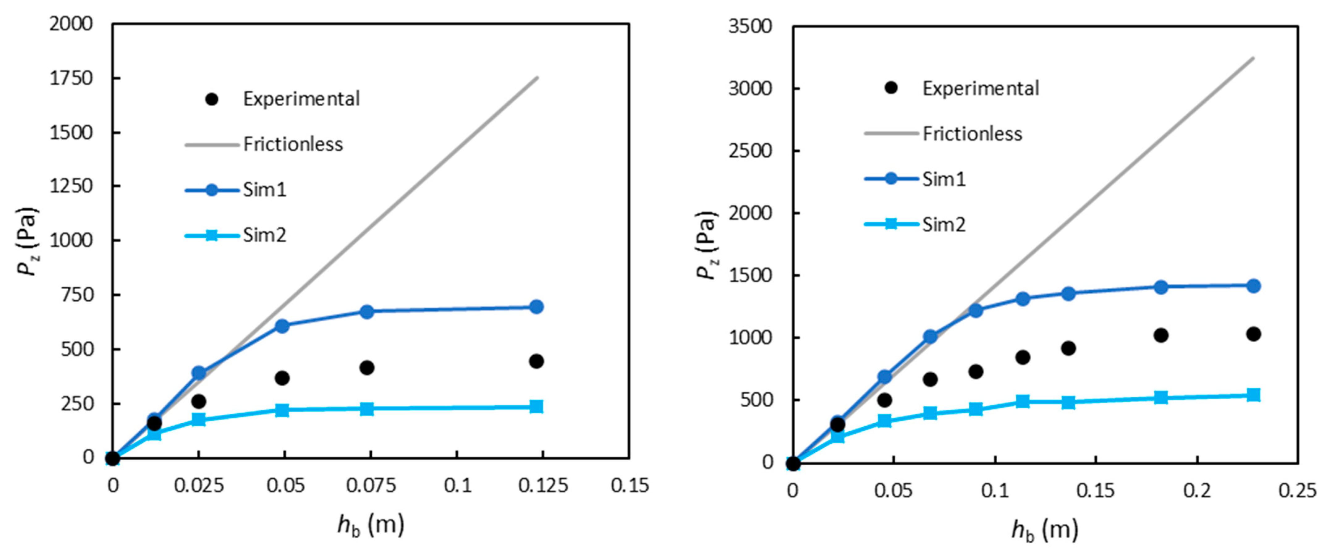
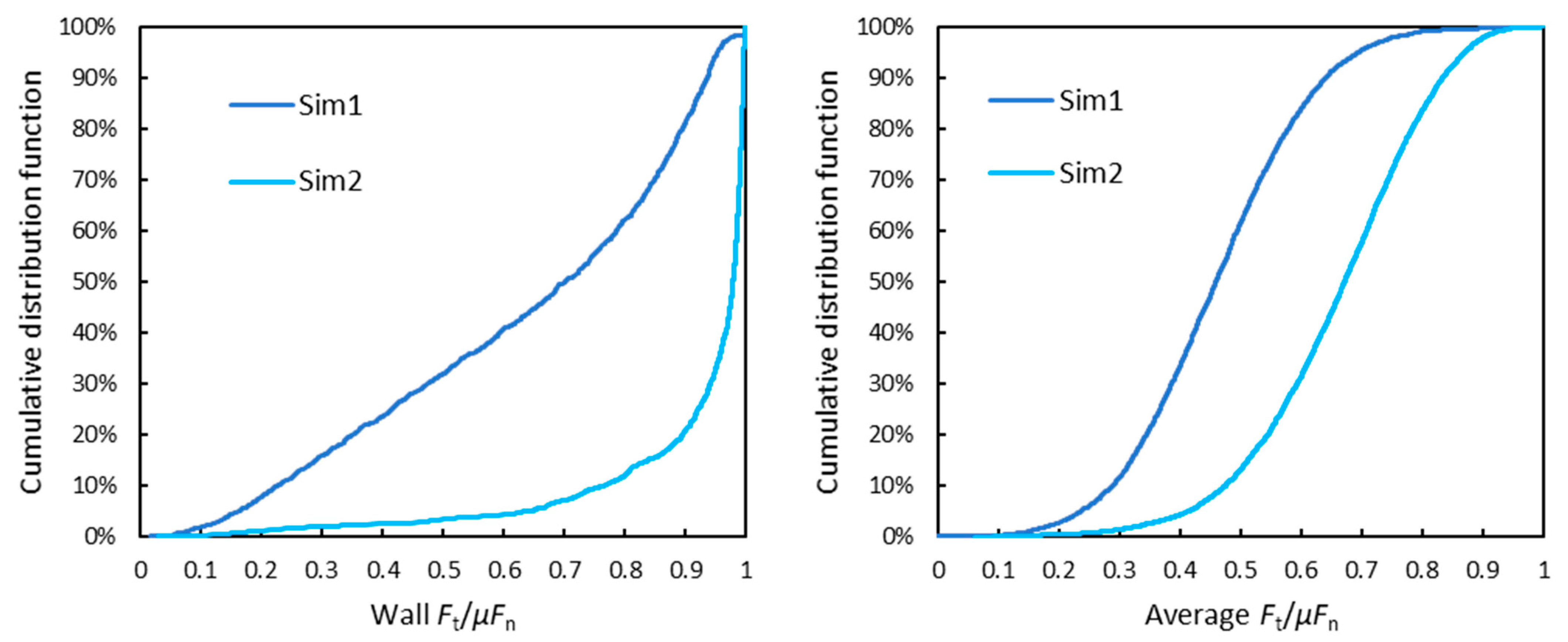
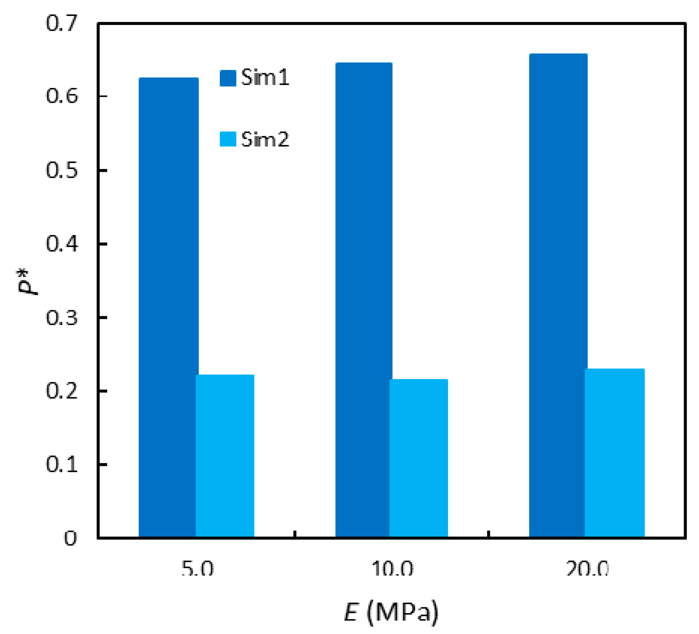
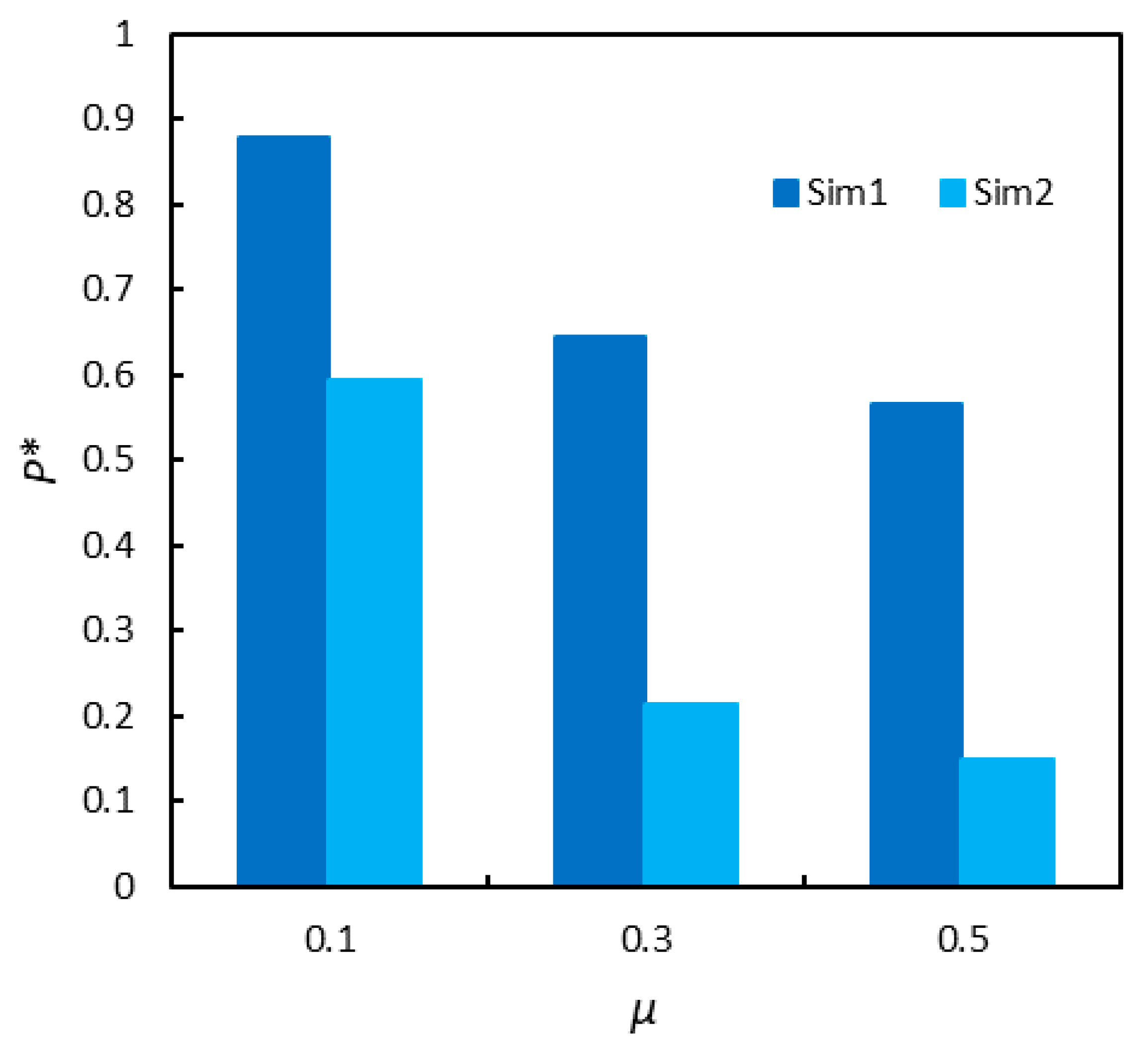
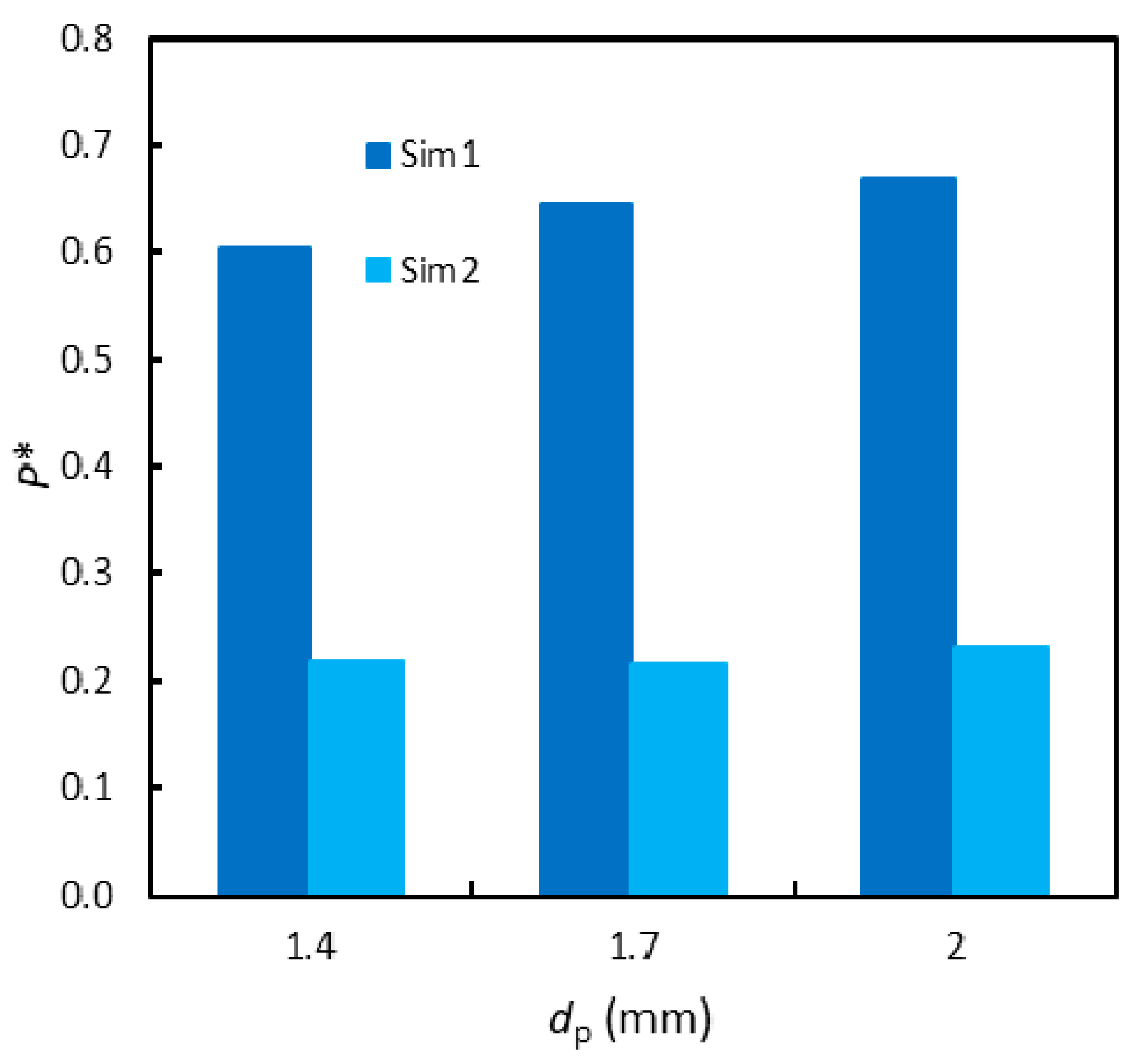
• When all particles had settled and stabilized, we extracted the values of F_n and F_t to analyze the internal stress distribution. The data related to this state are referred to as “Sim1”.
• Afterwards, the lateral wall was made move upwards with a speed of 1 mm/s for 1 s. This was done to partially reproduce two phenomena that may produce the same effect. The first is the expansion the wall in response to the pressure exerted by particles [8]. The second is the downward movement of the piston in contact with the balance, which was placed below the particles in the experiments [22]. Both phenomena make particles descend and reach the so‑called active state, thus increasing the particle-wall friction force, and reducing the pressure exerted on the bottom of the column. Increasing the particle-wall friction by moving the wall upwards is known as “friction mobilization” [17,18] and researchers have shown that wall movements in different directions lead to different friction variations. As Windows-Yule et al. [15] showed, the intensity of the wall vertical velocity is instead not very important, since even markedly different values produce rather similar results. Although this is clearly a simplified version of the physical phenomena, it can provide useful insights into the distribution of forces in the active state.
• After the wall had stopped moving and particles had stabilized, the values of F_n and F_t were investigated again. The data related to this state are referred to as “Sim2”.

Figure 2 provides a depiction of the falling process in the simulations.

As already mentioned, the FORTRAN code of MFiX had to be modified to extract relevant results. For example, MFiX does not normally provide information regarding solids pressure and interparticle forces. The goal was mostly achieved through the particle-based user variables DES_USR_VAR, which can be defined by the user to track specific information for each particle throughout the simulation. In particular, the module that calculates particle-wall collision forces (CALC_COLLISION_WALL) was updated to store the value of the particle-wall normal contact force in the vertical and radial direction. Due to the nature of these forces, the normal contact force in the vertical direction is not null only for particles touching the bottom of the column. Conversely, the normal contact force in the radial direction is not null only for particles touching the lateral wall of the column. The bottom (or lateral) pressure was then calculated by summing all the contact forces in the vertical (or radial) direction, and then dividing by the contact surface; the value was then saved as a ReactionRate. This is a misnomer, as anything can be saved as such, whether connected or not to chemical reactions. It is an easy way to store a variable and make it available for Monitors, which allow observation and storage of the values of a variable over the course of the simulation. With an analogous procedure, a user variable was also employed to calculate, for each particle, the ratio between the tangential force and its maximum value (that is, the product $\mu \left|\overrightarrow{F_{n,ij}}\right|$ as per the relevant equation), both for particle-particle (through the CALC_FORCE_DEM module) and particle-wall contacts (through the CALC_COLLISION_WALL module). Similarly, the two aforementioned modules were modified to calculate the coordination number. This was done by creating a further particle user variable and increasing its value by 1 at each contact force calculation. Finally, the fictitious movement of the lateral wall was instead obtained by modifying the module CALC_COLLISION_WALL and increasing by a desired amount the particle-wall relative tangential velocity for the desired time.

4. Results and Discussion

The first batch of simulations were aimed at understanding the capability of the approach to reproduce the trend of the solids pressure at the column bottom in response to an increasing bed height. Afterwards, we also performed a sensitivity analysis, with the purpose of assessing the extent of the influence that a variation of each parameter or model has on the results.

4.1. Analysis of the Stress Distribution

This section contains a discussion on the trends of the solids pressure for different bed heights (h_b). The comparison is based on two different systems: 1.7 mm glass particles in the 28 mm column and 5 mm glass particles in the 61 mm column. The simulation results are compared with experimental data and with the theoretical pressure in a frictionless column.

Figure 3 displays the trends of the bottom solids pressure for both columns. As explained in the previous section, the data for each bed height were obtained from a different simulation. An inspection of the plots permits inferring that both the Sim1 and Sim2 approaches can qualitatively reproduce the phenomenon. Although at shallow depths the solid pressure increases linearly, it becomes asymptotical for greater depths. The pressure remains roughly constant when the h_b/D ratio exceeds 2, which is also close to z = 2 z_sat in Janssen’s approach (provided that the product μK is about 0.25).

Moving onto a more quantitative analysis, it is clear that neither approach can provide a perfect fit of the experimental curve. The pressure obtained by simply letting particles fall (Sim1) is higher than the experimental data. Conversely, the data obtained after letting the walls move upwards (Sim2) is lower than the experimental data. Although this may look disappointing, we believe it is not an unexpected result. As already stated in the previous section, the experimental procedure entails several small phenomena that are hard to quantify and reproduce in simulations. Both the first and second approach are simplified versions of the experimental procedure, and do not exactly reproduce it. Moreover, our interest was more on reproducing the trends rather than perfectly simulating the numerical values: while the latter may actually have been feasible through a tuning of contact parameters and filling rate, we believe it would have been of low scientific interest and would not have necessarily reflected reality. Parameters aside, it is however encouraging that the experimental data lie between the two curves and may mean that what physically happens in the experiments is at least partially captured by the simulation approach.

Although the two plots of Figure 3 clearly show similar trends, it is better to assess the extent of this similarity. To this end, Figure 4 presents the results in a dimensionless form. The pressure is expressed as the ratio between the measured solid pressure at the bottom and the pressure that would be exerted on the bottom of a frictionless column (P*). Conversely, the bed height is divided by the column diameter (h_b/D). According to Janssen’s equations, the same P/P_sat values can be obtained for the same z/z_sat; for the same materials, the latter is proportional to the h_b/D ratio. Therefore, the larger the column is, the higher the particle bed needs to be to reach the asymptotical conditions. The figure proves that the effect is perfectly reproduced by MFiX in the tested case: for the same approach, the curves are practically identical. This is a valuable result, which confirms that the model can capture this phenomenon even when the geometry varies. It is also interesting to observe that while the experimental and Sim2 curves have a constant concavity, the Sim1 curves show a very small peak when the h_b/D ratio is about 1. This behavior is quite unexpected and may be caused by the filling method: the first particle that reach the bottom of the column have a high kinetic energy and may tend to pack in a very compact way, without being able to distribute the vertical stress on the lateral wall. With a more gradual filling process, the curve would probably lack the initial ascending phase and be more like the experimental one. Conversely, the curve of Sim2 is more similar to the experimental curve, which could confirm that the fictitious wall rise is not too different from what the particles actually experience in the physical setup.

A more in-depth investigation of the force and pressure distribution may provide other interesting details on the phenomenon. Figure 5 shows the trend of the solid pressure along the radial and vertical direction, obtained from the simulations of the 61 mm column. The data for the vertical pressure are the same of Figure 3, under the assumption that the vertical pressure at a certain depth only depends on the distance from the top of the bed. Conversely, those of the radial pressure were extracted from the simulation with the largest value of the bed height. To extract the pressure in the radial direction, the cylindrical column was divided into several slices in the horizontal direction, i.e., into several 1-cm-high cylinders. Then, the radial pressure was obtained by summing the normal particle-wall forces of all particles contained in each slice and dividing the value by the lateral surface area of the slice.

As already stated, the Janssen approach relies on the hypothesis that the ratio between these two pressures is a constant (K); to verify this, we calculated its value and included it in the graph (right axis). In the simple case of particles falling (Sim1, left plot), this seems roughly true, aside for the extreme points. There are indeed some oscillations, but K remains around a value of about 0.58. Since the friction coefficient µ is 0.3, the product µK is averagely 0.175, slightly lower than the commonly reported value of 0.2. The situation changes after the lateral wall has risen (Sim2, right plot). In this case, the radial pressure becomes larger than the vertical pressure. Its average value increases to 1.38, with a peak of 1.70. The average value of µK consequently increases to 0.41. From the theory [8], it is expected that a change in the state of the material (active or passive) leads to a variation of K. In fact, it should be smaller than 1 for the active state and larger than 1 for the passive state. The variation appears however opposite to what was expected from our preliminary considerations. A final note regarding this plot is that the values and trend of the pressure in radial direction for Sim1 and Sim2 are almost identical, compared to the abrupt variation of the vertical pressure caused by the increase of the friction force. Hence, also the variation of the trend of K is almost totally driven by the vertical pressure.

To further understand how the force distribution changes during the simulations, we decided to study the ratio between the tangent contact force F_t and its maximum value (µF_n). Figure 6 shows the data in the form of the cumulative distribution function of this ratio for all the simulated particles in the 61 mm column, in the same case of the previous graph. Specifically, in the left plot the ratio was only calculated for particle-wall contacts, while in the plot on the right we calculated the average of the ratio for all the contacts of each particle. As expected, the ratio is higher for particle-wall contacts: in these, F_t is oriented vertically and is indeed responsible for partially sustaining the weight of particles. Particle‑particle contact forces are instead oriented randomly. Nonetheless, when the particles are pushed towards an active state (Sim2), the ratio increases for both kinds of contacts. The effect is more evident for the wall contacts, in which the ration exceeds 0.9 for about 80% of the particles, with its average value being 0.918. This means that in this configuration the wall would not be able to provide a significantly higher friction force, unless the particle-wall normal force is increased as well.

It may also be useful to assess how the particle distribution and forces vary along the bed height. To this end, Figure 7 shows the variation of four relevant variables along the bed height: the coordination number, the particle volume fraction, the value for particle-wall contacts and all contacts of the ratio F_t/µF_n. These plots were obtained dividing the control volume in cylindrical slices with heights of 1 cm. The plots show a very abrupt variation of the coordination number (Figure 7a), which markedly decreases after the upward movement of the wall. This is in line with our previous hypothesis about the configuration of particle in Sim1: due to the initial high kinetic energy, lower particles pack in a very close way and do not manage to redistribute their weight on the lateral wall. Conversely, in Sim2 the contacts between particles decreases, and more so in the lower portion of the bed. This effect cannot be clearly observed for the particle volume fraction (Figure 7b): it reduces as well from Sim1 to Sim2, but its variation is much less apparent, and the slightly decreasing trend is preserved. For the F_t/µF_n ratios (Figure 7c,d), the considerations drawn for the previous Figure still apply. Additionally, it is interesting to observe that these two ratios display a more constant trend in Sim2, losing the local minimum that they both featured in the higher portion of the bed for Sim1.

A final aspect that we studied was the distribution of the normal stress on the base along the radial direction. To obtain the results, we divided the base in seven concentric slices of increasing radius, summed the normal contact forces of the particles lying on each slice (obtained with the procedure explained in the previous section) and divided the value by the surface area of the slice. Figure 8 depicts it for Sim1 and Sim2 in the 61 mm column. In both cases, the trend of the bottom stress is slightly concave. This is coherent with what Horabik and colleagues [17] recently reported for non-spherical particles when employing a distributed filling method. The wall movement does not significantly alter the shape of the curve: this is expected, since the upward movement causes a decrease of the bottom pressure near the lateral wall. The overall decrease of the average normal force is also coherent with the previously reported results.

To conclude this section, these simulations confirmed that the DEM approach provided by MFiX can correctly capture the behavior of solid pressure and friction at varying bed heights. We were not able to achieve a perfect match of the experimental data, but we believe this should be imputed to the impossibility of perfectly reproducing the experimental setup, rather than on limitations of the modeling tool.

4.2. Sensitivity Analysis

The second task of this work consisted of a sensitivity analysis. Its aims were to assess the influence of the sub-models and variables on the particle stress distribution and check that the modeling tool correctly considers them. To obtain results within an acceptable time, we based the analysis on the case of a 7.4-cm-high bed of 1.7 mm glass particles in the 28 mm column (unless otherwise stated). The choice was a compromise not to entail too many particles but also work in a situation in which the stress curve has already reached the plateau (as visible in Figure 3). The results are compared with the standard settings of the previous section, which have been summarized in Table 2. Results are presented through the dimensionless variable P*, which is the ratio between the measured solid pressure at the bottom and the pressure that would be exerted on the bottom of a frictionless column. This choice was due to the fact that P* showcases the most visible responses to the variation of the parameters and focusing on it allowed us to make the analysis more succinct and readable. As already depicted in the previous plots, in the chosen scenario the experimental value of P* was 0.397.

The first investigated aspect was the Young modulus E. For DEM simulations of poor-to-moderately packed systems, the particle stiffness is usually considered much lower than its actual value: this has been shown multiple times not to hinder the simulation results [40,41,42]. However, the present configuration is rather packed, so it is best not to decrease the stiffness excessively. When simulating glass particles with the Hertzian contact model, a value of the order of 10⁷ Pa is often employed for the Young modulus, as a compromise between computational complexity and accuracy [10,37,38,43]. Increasing the order of magnitude of this constant would have prevented us from achieving results within acceptable time. Thus, we only tried moderately modifying the value of the variable, to assess whether this would cause a vigorous friction difference. As Figure 9 shows, this was not the case. There seem to be a positive trend between the value of the particle stiffness and the bottom pressure, but the variation is too small to be appreciable. Moreover, while increasing the value of E should be more realistic, the P* values of Sim1 seem to further deviate from the experimental one.

Since the studied phenomena are mainly caused by the friction force, it may sound intuitive to tune the value of the friction coefficient µ. We selected values of 0.1 and 0.5 for this constant, in addition to the original value of 0.3; this range is common for DEM simulation of glass particles. Figure 10 shows the results. The pressure value obtained with a coefficient of 0.1 stands out the most: both approaches originate a pressure at the bottom that is higher than the experimental value. Clearly, this means that such a value leads to an underestimation of friction, which is thus unable to sustain a relevant portion of the weight of particles. The difference between 0.3 and 0.5 is still visible, but less intense. This is because the friction coefficient only affects the maximum value of the friction force: as shown in the previous section, for most particles the tangential force is far from its maximum. Indeed, when particles are simply let fall (Sim1), on average the particle-wall F_t/µF_n ratio is 0.45, 0.45 and 0.4 for the friction coefficients of 0.1, 0.3 and 0.5, respectively. After the lateral wall stops rising (Sim2), these values increase to 0.98, 0.85 and 0.64: they still are rather far from the maximum, aside for the lowest value of µ. In practical terms, while tuning the value of µ may appear as the most immediate practice to enhance the results, it may not be an effective path. If the constant cannot be measured experimentally, we think it is best to employ a standard value, such as 0.3 for glass particles.

Another relevant factor affecting the stress distribution is the way particles are placed inside the column. For example, Tixier and colleagues [44] showed experimentally that filling the column through the center or through the edges remarkably affects the bottom pressure. To check whether the model could capture this effect, we tried to vary the filling rate at which particles are poured inside the column. Operatively, we achieved this by varying the size of the hole through which particles pass to get into the column. Figure 11 displays the results, which prove that the effect is indeed captured by the modeling tool. If we look at the Sim1 results, it is clear that when particles fall at a higher rate, they generate a larger pressure at the bottom. The cause may be that when particles fall at a low rate, the force network manages to adapt to the new stresses and reach a sort of equilibrium status. Conversely, when the particles fall more intensely, this cannot happen, and each layer exerts the maximum vertical force. The effect is however only visible when the mass flux of particles is significant, while its influence is minimal when the particles fall at lower rates. Lower values were not tested due to the impossibility of achieving results within an acceptable time, while higher values were not tested as we deemed them as unrealistic (for the highest mass flux, the hole is almost as wide as the column). It shall be pointed out that in an industrial scenario, particles will likely be poured inside a silo through a small opening compared to the column width, so the higher values that we tested are quite unrealistic as well. Finally, it is interesting to observe that after the usual phase of the lateral wall moving upwards, the final bottom pressure is very similar in all cases. This implies that the movement of the wall completely erases the previous stress distribution and creates a new one, which is always roughly the same.

The final parameters that we tested can in no way be considered tunable to enhance the results, because they are intrinsic physical attributes of the system that are always known before setting up the simulations. Nonetheless, it was interesting to check whether the program could correctly respond to a variation of these. The first test regarded a limited variation of the particle diameter; Figure 12 displays the results. Both the results of Sim1 and Sim2 seem rather unaffected by its variation. This is coherent with the fact that the particle diameter does not appear in Janssen’s equations, so a marked influence of it is not expected. In this case, MFiX could correctly predict the independence of the results on this variable.

The observations of the previous paragraph partially change when the particle diameter is varied more sharply. Indeed, the experiments [22] had shown a visible difference in the bottom pressure when employing more heterogeneous particles. We simulated this by taking into account the 61 mm column, filled with 1.7 mm glass particles or 5 mm glass particles. Figure 13 depicts the results. Despite the already stated impossibility to exactly reproduce the physical reality, the model correctly captures the fact that the bottom pressure increases with the particle diameter (despite the slightly lower bed height). This effect is ascribable to wall effects: when the ratio between the particle diameter and the column diameter reaches a certain threshold, it is more difficult for horizontal force bridges to form, and thus the stress in the vertical direction becomes more intense. From a mathematical point of view, while the particle diameter does not appear in Janssen’s equations, the wall effect probably affects the value of K, leading to these results. It is interesting to observe that the 5 mm particles produce a higher pressure both in Sim1 and in Sim2, meaning that in this case the action of the rising wall does not suffice to align the two cases. These results are also coherent with the simulations of Zhao and colleagues [16], who showed that the wall effect can be very intense, especially when the D/d_p ratio is lower than 16.

The last studied variable was the particle density. Theoretically, it affects the magnitude of the pressure at the bottom, but not its trend as a function of the bed height, as it can be gathered from Equation (1) (dividing both members by P_sat). As Figure 14 depicts, the results provided by MFiX are coherent with these expectations, with P* remaining roughly constant even for very marked variation of the particle density. There actually seems to be a moderately decreasing trend, but its magnitude is so small within the whole density range that it can be neglected.

5. Conclusions

In this work, we employed the open-source program MFiX to analyze the stress distribution of solid particles placed inside vertical columns. The system was studied through DEM simulation, employing the Hertzian contact model and the Coulomb friction force. The aim of the work was to assess whether the program was able to correctly consider friction for static particles and provide a good description of the phenomenon, sometimes improperly known as the “Janssen effect”. To extract the required results, the program’s code was properly modified, as detailed in Section 3. Qualitatively, we observed that the program can reproduce the phenomenon, with the pressure of particles at the bottom showing an asymptotical behavior over certain values of the bed height. A perfect numerical match between experimental and simulated data could not be achieved, but we believe that this is expectable, since it is impossible to exactly reproduce the actual filling procedure and the response of the wall. Reassuringly, the experimental pressure values appear to be halfway between those obtained by simply letting particles fall and those obtained after making the lateral wall partially rise. The latter procedure is a way to partially reproduce what may happen in reality, with the wall partially expanding and particles reaching the so‑called active state. The results of the DEM simulations show that most particles are far from experiencing the maximum friction force, although this majority is lessened by the wall’s rise. Moreover, the data confirm that the ratio K is not always constant, contrarily to what Janssen originally hypothesized.

A further sensitivity analysis allowed us to confirm the suitability of MFiX in the way all the simulation parameters are considered. Most notably, an increase of the friction coefficient may not always produce the desired results, since it only affects the theoretical maximum friction force. The particle filling rate is also an important factor, with very high values eliminating the asymptotical effect. The filling methodology is very likely to be the most relevant factor to achieve the expected results, but due to the complexity of this aspect a more detailed study on this is left for future works. In conclusion, this DEM modeling approach can correctly capture the behavior of the friction force when particles are static. We will further apply it to test whether it can also well predict the influence of the friction force when particles are about to shift from a static to a moving state, i.e., in the fluidization of heterogeneous particles.

References

1. Cundall, P.A.; Strack, O.D.L. A discrete numerical model for granular assemblies. Géotechnique 1979, 29, 47–65. [Google Scholar] [CrossRef]
2. Guo, Y.; Curtis, J.S. Discrete Element Method Simulations for Complex Granular Flows. Annu. Rev. Fluid Mech. 2015, 47, 21–46. [Google Scholar] [CrossRef]
3. Zhou, Z.Y.; Kuang, S.B.; Chu, K.W.; Yu, A.B. Discrete particle simulation of particle–fluid flow: Model formulations and their applicability. J. Fluid Mech. 2010, 661, 482–510. [Google Scholar] [CrossRef]
4. Ibrahim, A.; Meguid, M.A. Coupled Flow Modelling in Geotechnical and Ground Engineering: An Overview. Int. J. Geosynth. Ground Eng. 2020, 6, 39. [Google Scholar] [CrossRef]
5. Di Felice, R.; Scapinello, C. The transition from the fixed to the fluidised state of binary-solid liquid beds. Chem. Eng. Sci. 2010, 65, 5187–5192. [Google Scholar] [CrossRef]
6. Janssen, H.A. Versuche über Getreidedruck in Silozellen. Z. Ver. Dtsch. Ing. 1895, 39, 1045. [Google Scholar]
7. Sperl, M. Experiments on corn pressure in silo cells—Translation and comment of Janssen’s paper from 1895. Granul. Matter 2006, 8, 59–65. [Google Scholar] [CrossRef] [Green Version]
8. Nedderman, R.M. Statics and Kinematics of Granular Materials; Cambridge University Press: Cambridge, UK, 1992. [Google Scholar]
9. Peng, Z.; Li, R.; Jiang, Y. Stress distribution along sidewall of a granular column: Local fluctuation and global determination. Phys. A Stat. Mech. Its Appl. 2019, 526, 120865. [Google Scholar] [CrossRef]
10. Zhao, H.; An, X.; Wu, Y.; Qian, Q. DEM modeling on stress profile and behavior in granular matter. Powder Technol. 2018, 323, 149–154. [Google Scholar] [CrossRef]
11. Ramírez-Gómez, Á. The discrete element method in silo/bin research. Recent advances and future trends. Part. Sci. Technol. 2020, 38, 210–227. [Google Scholar] [CrossRef]
12. Žurovec, D.; Hlosta, J.; Nečas, J.; Zegzulka, J. Monitoring bulk material pressure on bottom of storage using DEM. Open Eng. 2019, 9, 623–630. [Google Scholar] [CrossRef]
13. Acevedo, M.; Zuriguel, I.; Maza, D.; Pagonabarraga, I.; Alonso-Marroquin, F.; Hidalgo, R.C. Stress transmission in systems of faceted particles in a silo: The roles of filling rate and particle aspect ratio. Granul. Matter 2014, 16, 411–420. [Google Scholar] [CrossRef]
14. Qian, Q.; Wang, L.; An, X.; Wu, Y.; Wang, J.; Zhao, H.; Yang, X. DEM simulation on the vibrated packing densification of mono-sized equilateral cylindrical particles. Powder Technol. 2018, 325, 151–160. [Google Scholar] [CrossRef]
15. Windows-Yule, C.R.K.; Mühlbauer, S.; Cisneros, L.A.T.; Nair, P.; Marzulli, V.; Pöschel, T. Janssen effect in dynamic particulate systems. Phys. Rev. E 2019, 100, 1–7. [Google Scholar] [CrossRef]
16. Zhao, H.; An, X.; Wu, Y.; Yang, X. Microscopic analyses of stress profile within confined granular assemblies. AIP Adv. 2018, 8. [Google Scholar] [CrossRef] [Green Version]
17. Horabik, J.; Parafiniuk, P.; Molenda, M. Stress profile in bulk of seeds in a shallow model silo as influenced by mobilisation of particle-particle and particle-wall friction: Experiments and DEM simulations. Powder Technol. 2018, 327, 320–334. [Google Scholar] [CrossRef]
18. Vivanco, F.; Mercado, J.; Santibáñez, F.; Melo, F. Stress profile in a two-dimensional silo: Effects induced by friction mobilization. Phys. Rev. E 2016, 94, 022906. [Google Scholar] [CrossRef]
19. Wiącek, J.; Stasiak, M.; Parafiniuk, P. Effective elastic properties and pressure distribution in bidisperse granular packings: DEM simulations and experiment. Arch. Civ. Mech. Eng. 2017, 17, 271–280. [Google Scholar] [CrossRef]
20. Garg, R.; Galvin, J.; Li, T.; Pannala, S. Open-source MFiX-DEM software for gas-solids flows: Part I-Verification studies. Powder Technol. 2012, 220, 122–137. [Google Scholar] [CrossRef]
21. Garg, R.; Galvin, J.; Li, T.; Pannala, S. Documentation of Open-Source MFiX–DEM Software for Gas-Solids Flows. Available online: https://mfix.netl.doe.gov/documentation/demdoc2010.pdf (accessed on 25 December 2020).
22. Di Felice, R.; Scapinello, C. On the interaction between a fixed bed of solid material and the confining column wall: The Janssen approach. Granul. Matter 2010, 12, 49–55. [Google Scholar] [CrossRef]
23. Lungu, M.; Siame, J.; Mukosha, L. Comparison of CFD-DEM and TFM approaches for the simulation of the small scale challenge problem 1. Powder Technol. 2020, 378, 85–103. [Google Scholar] [CrossRef]
24. Garcia-Gutierrez, L.M.; Hernández-Jiménez, F.; Cano-Pleite, E.; Soria-Verdugo, A. Improvement of the simulation of fuel particles motion in a fluidized bed by considering wall friction. Chem. Eng. J. 2017, 321, 175–183. [Google Scholar] [CrossRef]
25. Gao, X.; Li, T.; Rogers, W.A.; Smith, K.; Gaston, K.; Wiggins, G.; Parks, J.E. Validation and application of a multiphase CFD model for hydrodynamics, temperature field and RTD simulation in a pilot-scale biomass pyrolysis vapor phase upgrading reactor. Chem. Eng. J. 2020, 388, 124279. [Google Scholar] [CrossRef]
26. Fullmer, W.D.; Musser, J. CFD-DEM solution verification: Fixed-bed studies. Powder Technol. 2018, 339, 760–764. [Google Scholar] [CrossRef]
27. Zinani, F.; Philippsen, C.G.; Indrusiak, M.L.S. Numerical study of gas–solid drag models in a bubbling fluidized bed. Part. Sci. Technol. 2018, 36, 1–10. [Google Scholar] [CrossRef]
28. Adepu, M.; Chen, S.; Jiao, Y.; Gel, A.; Emady, H. Wall to particle bed contact conduction heat transfer in a rotary drum using DEM. Comput. Part. Mech. 2020, 1–11. [Google Scholar] [CrossRef]
29. Xu, Y.; Li, T.; Lu, L.; Tebianian, S.; Chaouki, J.; Leadbeater, T.W.; Jafari, R.; Parker, D.J.; Seville, J.; Ellis, N.; et al. Numerical and experimental comparison of tracer particle and averaging techniques for particle velocities in a fluidized bed. Chem. Eng. Sci. 2019, 195, 356–366. [Google Scholar] [CrossRef]
30. Ansari, A.; Mohaghegh, S.D.; Shahnam, M.; Dietiker, J.F. Modeling Average Pressure and Volume Fraction of a Fluidized Bed Using Data-Driven Smart Proxy. Fluids 2019, 4, 123. [Google Scholar] [CrossRef] [Green Version]
31. Miramontes, E.; Love, L.J.; Lai, C.; Sun, X.; Tsouris, C. Additively manufactured packed bed device for process intensification of CO2 absorption and other chemical processes. Chem. Eng. J. 2020, 388, 124092. [Google Scholar] [CrossRef]
32. Yu, Y.; Zhao, L.; Li, Y.; Zhou, Q. A Model to Improve Granular Temperature in CFD-DEM Simulations. Energies 2020, 13, 4730. [Google Scholar] [CrossRef]
33. Syamlal, M.; Rogers, W.; O’Brien, T.J. MFiX Documentation Theory Guide; Department of Energy: Oak Ridge, TN, USA, 1993; Volume 1004.
34. Di Renzo, A.; Di Maio, F.P. Comparison of contact-force models for the simulation of collisions in DEM-based granular flow codes. Chem. Eng. Sci. 2004, 59, 525–541. [Google Scholar] [CrossRef]
35. Paulick, M.; Morgeneyer, M.; Kwade, A. Review on the influence of elastic particle properties on DEM simulation results. Powder Technol. 2015, 283, 66–76. [Google Scholar] [CrossRef]
36. Alaci, S.; Muscă, I.; Pentiuc, Ș.-G. Study of the Rolling Friction Coefficient between Dissimilar Materials through the Motion of a Conical Pendulum. Materials 2020, 13, 5032. [Google Scholar] [CrossRef] [PubMed]
37. Xiang, J.; McGlinchey, D.; Latham, J.P. An investigation of segregation and mixing in dense phase pneumatic conveying. Granul. Matter 2010, 12, 345–355. [Google Scholar] [CrossRef]
38. Zhang, M.; Yang, Y.; Zhang, H.; Yu, H.-S. DEM and experimental study of bi-directional simple shear. Granul. Matter 2019, 21, 24. [Google Scholar] [CrossRef]
39. Yang, R.Y.; Zou, R.P.; Yu, A.B. Numerical study of the packing of wet coarse uniform spheres. AIChE J. 2003, 49, 1656–1666. [Google Scholar] [CrossRef]
40. Marchelli, F.; Moliner, C.; Bosio, B.; Arato, E. A CFD-DEM sensitivity analysis: The case of a pseudo-2D spouted bed. Powder Technol. 2019, 353, 409–425. [Google Scholar] [CrossRef]
41. Bakshi, A.; Shahnam, M.; Gel, A.; Li, T.; Altantzis, C.; Rogers, W.; Ghoniem, A.F. Comprehensive multivariate sensitivity analysis of CFD-DEM simulations: Critical model parameters and their impact on fluidization hydrodynamics. Powder Technol. 2018, 338, 519–537. [Google Scholar] [CrossRef]
42. Coetzee, C.J. Review: Calibration of the discrete element method. Powder Technol. 2017, 310, 104–142. [Google Scholar] [CrossRef]
43. Wu, Y.; Hou, Q.; Dong, K.; Yu, A. Effect of packing method on packing formation and the correlation between packing density and interparticle force. Particuology 2020, 48, 170–181. [Google Scholar] [CrossRef]
44. Tixier, M.; Pitois, O.; Mills, P. Experimental impact of the history of packing on the mean pressure in silos. Eur. Phys. J. E 2004, 14, 241–247. [Google Scholar] [CrossRef] [PubMed]
Figure 1. DEM simulations of particles falling through a slit in a commercial program (left) and MFiX (right): (a) particles falling; (b) all particles have fallen; (c) the system has stabilized.
Processes 09 00060 g001
Figure 2. Different phases of particle settling at the beginning of the simulations (28 mm column, 7.4 cm bed height).
Processes 09 00060 g002
Figure 3. Solids pressure at different bed depths: 1.7 mm glass particles in the 28 mm column (left) and 5 mm glass particles in the 61 mm column (right).
Processes 09 00060 g003
Figure 4. Dimensionless version of the two previous plots, for both columns.
Processes 09 00060 g004
Figure 5. Solid pressure in the radial and vertical direction along the height of the column for Sim1 (left plot) and Sim2 (right plot).
Processes 09 00060 g005
Figure 6. Cumulative distribution of the ratio between the tangent force and its maximum value for particle‑wall contacts (left) and all contacts (right).
Processes 09 00060 g006
Figure 7. Variation along the vertical coordinate of the coordination number (a), solids volume fraction (b), particle-wall Ft/µFn ratio (c) and overall Ft/µFn ratio (d).
Processes 09 00060 g007
Figure 8. Radial trend of the normal stress at the bottom of the column.
Processes 09 00060 g008
Figure 9. Pressure at the bottom of the column upon varying the Young modulus.
Processes 09 00060 g009
Figure 10. Pressure at the bottom upon varying the friction coefficient.
Processes 09 00060 g010
Figure 11. Pressure at the bottom upon varying the falling particle flux.
Processes 09 00060 g011
Figure 12. Pressure at the bottom upon slightly varying the particle diameter.
Processes 09 00060 g012
Figure 13. Pressure at the bottom in the 61 mm column upon varying the particle diameter.
Processes 09 00060 g013
Figure 14. Pressure at the bottom upon varying the particle density.
Processes 09 00060 g014