An Autoencoder Gated Recurrent Unit for Remaining Useful Life Prediction

Abstract

With the development of smart manufacturing, in order to detect abnormal conditions of the equipment, a large number of sensors have been used to record the variables associated with production equipment. This study focuses on the prediction of Remaining Useful Life (RUL). RUL prediction is part of predictive maintenance, which uses the development trend of the machine to predict when the machine will malfunction. High accuracy of RUL prediction not only reduces the consumption of manpower and materials, but also reduces the need for future maintenance. This study focuses on detecting faults as early as possible, before the machine needs to be replaced or repaired, to ensure the reliability of the system. It is difficult to extract meaningful features from sensor data directly. This study proposes a model based on an Autoencoder Gated Recurrent Unit (AE-GRU), in which the Autoencoder (AE) extracts the important features from the raw data and the Gated Recurrent Unit (GRU) selects the information from the sequences to forecast RUL. To evaluate the performance of the proposed AE-GRU model, an aircraft turbofan engine degradation simulation dataset provided by NASA was used and a comparison made of different recurrent neural networks. The results demonstrate that the AE-GRU is better than other recurrent neural networks, such as Long Short-Term Memory (LSTM) and GRU.

1. Introduction

Industry 4.0 depends on automated, smart factories, and employs sensor data and the methods of big data analysis, in the expectation that the equipment in the factory will operate automatically and self-correct to improve the product yield [1]. Sensor-related data are collected during the manufacturing processes, such as temperature, pressure, power, humidity, and chemical analysis for equipment monitoring [2,3]. These temporal patterns represent the equipment condition, and poor product quality is often associated with abnormal changes of environment or inappropriate operation settings [4]. Equipment condition can be recorded by sensor data from the past and kept as time series data. When analyzing equipment sensor data, not only the large amount of data recorded should be considered, but also the time series characteristics. The idea of a smart factory is to link and intellectualize the manufacturing process. In the past, automation merely used machines to improve production efficiency, yield, and reduce costs, but intelligence further applies technologies such as the IoT sensor, to monitor and control production lines. The combination of cloud computing, data analysis, and software and hardware integration is also an important part of intelligence. Machines communicate with automation equipment [5]. However, there are numerous parameters in the smart factory, and the data are often highly correlated between equipment and processes. Therefore, the analysis must go beyond a single stage in the equipment or process, and be comprehensive.

Equipment maintenance methods are divided into the following three types: (1) repair maintenance [6]; (2) preventive maintenance [7]; (3) predictive maintenance [8]. Corrective maintenance is a method of maintenance that is performed after some or all of the equipment fails. The most common equipment maintenance application is preventive maintenance, also known as scheduled maintenance, which carries out machine inspections, component replacement and other maintenance at prescribed times. Predictive maintenance is an equipment maintenance method based on the condition of the machine. It predicts the time when the machine may be damaged according to the development trend of the past.

Predictive Maintenance (PdM) has been used to monitor the historical health status of equipment and make timely adjustments to the equipment, which is quite different from the methods of routine maintenance employed in the past. PdM not only saves unnecessary costs, but also allow early repairs when the equipment is about to break down. It can avoid unpredictable machine stoppages caused by unexpected breakdown and improper operation. Remaining Useful Life (RUL) is an important indicator in PdM. The definition of device or system RUL is the period from the current state to the time when the device begins to operate abnormally [9]. There are two types of RUL prediction: model-based and data-driven [10]. The model-based method establishes the model based on the historical trend of equipment. Generally, model-based methods perform better than data driven methods when there is little historical data. Data-driven methods use the health status data and data collected by sensors. For modeling, the collected data must be closely related to the device status. The advantage of data-driven methods is that the algorithm is based on learning the correlation between input and output data. If there are sufficient data, the stability and accuracy of data-driven methods are better than model-based methods

RUL prediction can be described as a time series forecasting problem. The main purpose of time series forecasting is to build models from historical records and predict future situations. Time series forecasting can be divided into statistical models, machine learning models and deep learning models. Common statistical models include Autoregression (AR), Moving Average (MA), Autoregressive Moving Average (ARMA), and Autoregressive Integrated Moving Average (ARIMA). Machine learning builds a function or model to detect patterns in training samples and then uses these patterns for prediction [11]. Support Machine Vector (SVM) [12], Random Forest (RF) [13], Extreme Gradient Boosting (XGB) [14] are representative machine learning algorithms for time series forecasting, but it is difficult to design an effective machine learning algorithm without substantial knowledge of the data [15]. In addition, the existing methods for analyzing time series data need pre-processing based on experience, which causes some losses of information. With improved process technology and more sensors, few existing methods can handle multi-sensor data, which is likely to cause misjudgment or missed detection.

Deep learning methods are preferred to predict and analyze time series data without predefined features. Deep learning is a branch of machine learning based on artificial neural networks with representation learning [16,17,18], which can learn the key information to make a response by using many hidden layers integrated in the network. The main difference between deep learning and machine learning is feature extraction. Usually, the features of machine learning are manually selected in advance; deep learning not only identifies features through model training, but is also much better than other algorithms at calculating results. Makridakis et al. [19] compare several time series analysis methods on the M3-Competition dataset. Most of the machine learning and deep learning algorithms perform better than traditional statistic methods. Alfred et al. [20] demonstrated that algorithms based on neural networks are more efficient in learning time series data than other algorithms.

Feature extraction is an important data pre-processing method in machine learning for high prediction accuracy. In the past, the dimension reduction of most data features was accomplished through Principal Component Analysis (PCA). PCA retains the maximum variation of features by projecting variables into another space to represent the original complete data with fewer features, to achieve the effect of data dimension reduction. The difference between PCA and Autoencoder (AE) is that AE is a non-linear dimension reduction method [21], and an unsupervised training method. First, the model compresses the original data through the encoder structure, and then restore the compressed data through the decoder. The AE rebuilds the original data with fewer features for data representation [22]. It can compress the key information of high dimensional input data into low dimensional features. AE is often used for feature extraction and dimensional reduction in time series forecasting problems [23]. Moreover, machine learning methods required manual selection of features. The quality of the features affected the models’ results. Deep learning has the ability to automatically extract features. It can reduce the time spent on feature engineering and help experts to make decisions. Most of the relevant studies on RUL prediction use deep learning as a prediction model, which not only can save time in selecting features, but also makes prediction results much better than traditional machine learning models.

Recurrent Neural Networks (RNN) are a deep learning model that deals specifically with time series data and can select important features from equipment sensors. Long Short-Term Memory networks (LSTM) is a variant of RNN [24]. For example, Zhang et al. [25] constructed an LSTM model to predict the RUL of lithium batteries, predicting after how many cycles of fully charge and discharge the capacity will be lower than the normal threshold, based on the historical decline rate of capacity. Heimes [9] set the maximum remaining engine life at 130 on the PHM08 data set, and predicted the RUL using an RNN model. Zhang et al. [25] also constructed an LSTM model to predict the RUL of the jet engine. One hundred jet engines were used as training data and 100 were used as testing data. Each jet engine has 24 features that record the sensor value from normal to fault, and the RUL are predicted by the change in these values. Mathew et al. [26] predict the RUL of jet engines, using 24 parameters of the original data and comparing ten machine learning methods (Linear Regression, Decision Tree, SVM, Random Forest, KNN, K-means, Gradient Boost, Adaboost, Deep Learning, ANOVA), and verify the validity of the model through RMSE. Zheng et al. [27] used an LSTM model to predict the RUL on C-MAPSS data set, PHM08 data set, and Milling data set. The LSTM model is better than the other models. Chen et al. [28] proposed a two-phase model for RUL prediction by Kernel Principal Component Analysis (KPCA) and Gated Recurrent Unit (GRU), respectively. To the best of our knowledge, little research has integrated AE and GRU for RUL prediction.

This study develops an Autoencoder Gated Recurrent Unit (AE-GRU) model to predict the RUL of equipment. In particular, AE is used to select features, and then the correlation between sensors is found through the GRU model, and the RUL is predicted by Multi-Layer Perception (MLP) model. The first part is the Autoencoder (AE) model which is composed of an encoder and decoder. The second part is the GRU model which is a type of RNN that can deal with time series data. The GRU model finds key information in historical sensor data in combination with the MLP model. The MLP model calculates the extracted information and combines with the backpropagation algorithm to predict the RUL effectively.

2. Literature Review

Time series are statistical data, arranging events or data in order of their occurrence. The main purpose of time series forecasting is to build models from historical records and predict future situations.

2.1. Recurrent Neural Networks

RNN is the most common time series analysis method in deep learning. The main difference between RNN and general neural network is that the neurons of RNN between hidden layers are not independent, but influence each other. The neurons of RNN also operate in order. The neurons of the recurrent neural network have the function of temporarily storing memory. The previously input data will be temporarily stored in the internal memory, so the neuron can have different output values according to the previous state. However, in the training of RNN, too many hidden layer neuron weights will cause the problem of gradient vanish because of the heavy calculation, which will let the gradient descent method stay at the local minimum. The traditional neural network has different parameters to be learned in each hidden layer, but the parameters of the RNN only have different inputs. This feature greatly reduces the training burden of the model.

LSTM solves the problem of the gradient vanish in the random gradient descent in recurrent neural networks. The biggest difference between the LSTM and RNN is that each neuron of LSTM has a control gate function, which is input, forget, and output. These gates have their own weights. The calculation of the weights after data input determines whether the switches are turned on or off. The input gate controls whether data can be written to the memory space, and the forget gate determines whether the contents of the previous memory space are retained. The output gate controls whether the memory space operation result can be output. Although adding these gates to each neuron generates more weight to be calculated, it can solve the problem of gradient vanish found in the recurrent neural network.

Figure 1 is a diagram of the LSTM network unit architecture, and the related formulas are shown as Equations (1)–(6). The LSTM unit will receive the input vector $x_t$ and the output $h_{t-1}$. Each unit contains four gates (i, g, f, o) and a cell. x is the input vector of this layer, h is the output vector, ⨀ is the element-wise multiplication. W is the weight matrix, b is an error vector, and (i, f, o, g, c) represents input gate, forget gate, output gate, cell input, and cell activation respectively. The forget gate controls how much information each memory unit needs to forget, the input gate controls how much new information each memory unit adds, and the output gate controls how much information each memory unit outputs. The cell input is the information input of the current time and the information of the previous time. Cell activation controls the whether the input gate and forget gate information can be obtained.

$$i_t=sigmoid\left({\mathit{W}}_{xi}{\mathit{x}}_t+{\mathit{W}}_{hi}{\mathit{h}}_{t-1}+{\mathit{b}}_i\right)$$

(1)

$$f_t=sigmoid\left({\mathit{W}}_{xf}{\mathit{x}}_t+{\mathit{W}}_{hf}{\mathit{h}}_{t-1}+{\mathit{b}}_f\right)$$

(2)

$$o_t=sigmoid\left({\mathit{W}}_{xo}{\mathit{x}}_t+{\mathit{W}}_{ho}{\mathit{h}}_{t-1}+{\mathit{b}}_o\right)$$

(3)

$$g_t=tanh\left({\mathit{W}}_{xg}{\mathit{x}}_t+{\mathit{W}}_{hg}{\mathit{h}}_{t-1}+{\mathit{b}}_g\right)$$

(4)

$$c_t=f_t\odot c_{t-1}+i_t\odot g_t$$

(5)

$$h_t=\tanh \left(c_t\right)\odot o_t$$

(6)

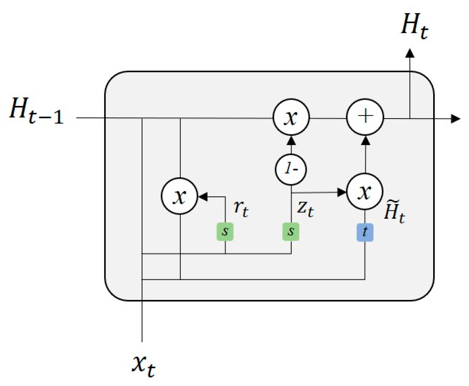
The gated recurrent unit (GRU) is a variant of LSTM [29]. As shown in Figure 2, (z, r, H, $\tilde{H}$) are update gate, reset gate, activation, and candidate activation respectively. The detailed formulas are shown an Equations (7)–(10). The update gate is used to control how much historical information and new information needs to be forgotten in the current state. The reset gate is used to control how much information is available from the candidate state. The candidate activation can be regarded as the new information at the current time. The reset gate is used to control how much historical information needs to be retained. The activation is generated by the update gate and candidate activation. The update gate in activation controls how much new and old information is retained. New information and old information have a complementary relationship. If a lot of new information is retained, the old information considered will be less, and vice versa.

$$z_t=sigmoid\left({\mathit{W}}_{xz}{\mathit{x}}_t+{\mathit{W}}_{hz}{\mathit{h}}_{t-1}+{\mathit{b}}_z\right)$$

(7)

$$r_t=sigmoid\left({\mathit{W}}_{xr}{\mathit{x}}_t+{\mathit{W}}_{hr}{\mathit{h}}_{t-1}+{\mathit{b}}_r\right)$$

(8)

$${\tilde{H}}_t=\tanh \left({\mathit{W}}_{x\tilde{H}}{\mathit{x}}_t+{\mathit{W}}_{H\tilde{H}}{\mathbf{r}}_t⨀H_{t-1}+{\mathit{b}}_{\tilde{H}}\right)$$

(9)

$$H_t=z_t⨀H_{t-1}+\left(1-z_t\right)⨀{\tilde{H}}_t$$

(10)

GRU simplifies the input gate and forget gate of LSTM into an update gate, and combines the cell states and hidden states together. Therefore, the GRU unit retains the advantages of LSTM, and further reduces the model training time by reducing the parameters in the model. According to the analysis results in [30], the results of the RNN model are poor and the results of GRU and LSTM are similar, and better than RNN. However, the GRU has fewer parameters than LSTM, so the trend in deep learning models applied to time series analysis is toward GRU.

In view of the excellent feature extraction performance of AE, and the fast calculation advantage of GRU, in this study the RUL prediction model works by extracting the important features from the original data using AE. After pre-processing of the extracted features, the GRU model and DNN (deep fully connected neural networks) are applied to predict the RUL.

2.2. RNN Applications in Time Series Forecasting

Chen et al. [31] performed a prediction of mechanical state (PMS), and extracted the collected sensor data of the machine through the feature extraction of empirical mode decomposition. This method makes the unstable signal slightly stable for building the LSTM model. Zheng et al. [32] predicts the short-term power system load capacity, the time range collected from a few hours to several weeks. The characteristics of power system load data are non-linear, non-stationary, and non-seasonal, so the research applies an LSTM model to solve this problem. ElSaid et al. [33] applied an LSTM model to predict aircraft engine vibration and predicted aircraft engine vibration values in the next 5, 10, and 20 s. 76 parameters are recorded in the aircraft flight data recorder. Fifteen key features were selected by experts with a professional background. The features were normalized to make the values range between 0 and 1, and used to make predictions. Cenggoro and Siahaan [34] constructed a DLSTM (Deep Long Short-Term Memory) neural network to predict traffic flow. The input layer had 5 input values, there were 5 hidden layers, and each hidden layer had 100 neurons. Bao et al. [35] conducted a stock price prediction. The stock price prediction is divided into three stages. Stage one applied a wavelet transform algorithm to remove noise from the original data. Stage two stacks AEs to reduces the data dimensions and picks out features automatically. Stage three applies an LSTM model to make predictions. Zhang et al. [36] divided Sea Surface Temperature (SST) into two part to make the prediction. The first part is short-term forecasting, which predicts the SST after 1 and 3 day. The second part is long-term forecasting, which predicts the weekly average and monthly average of SST. It finds the relationship between sequences through LSTM, and then make the prediction through the fully connected layer. How et al. [37] uses the angle changes on different motion sensors of the NAO robot to classify the current actions of the robot through an LSTM model. Truong et al. [38] construct an LSTM model to identify changes in human type and object type, and even predict possible human actions through the action combinations. Kuan et al. [39] constructed an MS-GRU (multilayered self-normalizing gated recurrent units) model. It has good results in predicting power loading. Zhang and Kabuka [40] used the GRU model to predict the traffic volume. The training data included the historical weather data 100 h previously to predict the traffic volume in the next 12 h. It was found that weather conditions can improve the prediction accuracy.

3. Research Framework

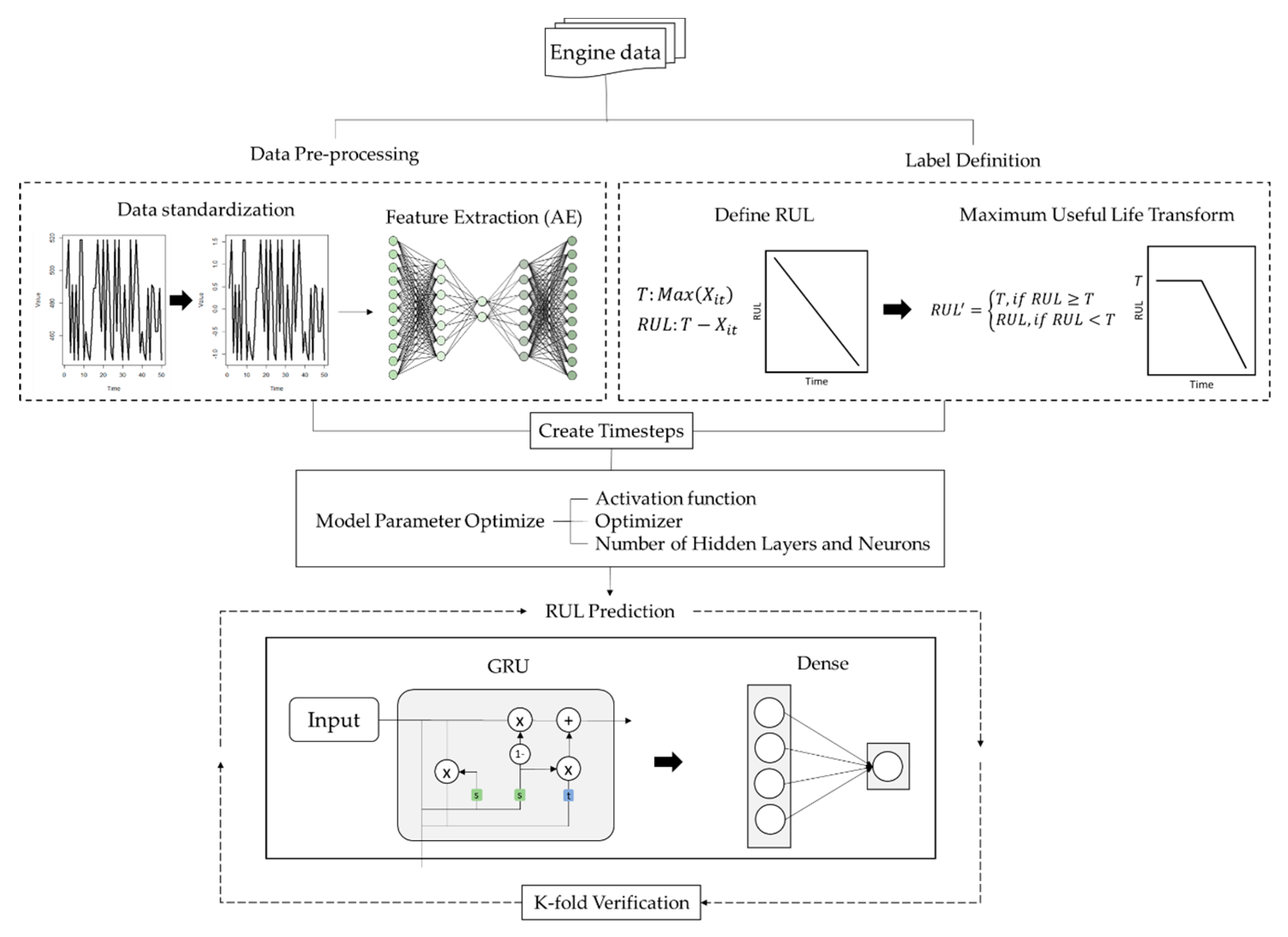
This study constructs an AE-GRU model for RUL prediction to increase equipment life, reduce unexpected harm caused by sudden shutdown of machinery, and improve the reliability of system operation. The proposed AE-GRU includes the steps of data pre-processing, feature extraction, and RUL prediction as shown in Figure 3. The data pre-processing step first defines the engine life to predict the exact RUL of the engine, and then standardizes the data to avoid errors caused by different scales of the data. It then uses the deep learning autoencoder model to extract the features of the original data. GRU is specialized in processing time series related data, and considers the changes of historical characteristics. The data is converted from 2D to 3D; the new dimension is the time data. The last step of data processing is to change the value range of the RUL. Because the original data is linearly decreasing, the results in model training and prediction are not optimal. Finally, the RUL expectancy is predicted through the GRU model and a fully-connected layer neural network.

The symbols used in this research are defined as follows:

• $N:numberofengines$
• $S:numberofsensors$
• $n:lengthofsensingdata$
• $Y:numberofneurons$
• $L:numberofhiddenlayers$
• $W:weight$
• $b:errorvector$
• $Features:Newfeaturesafterextraction$
• $X_{ij}:thesensingdataofthejthsensor\in theithengine;i=1\dots N,j=1\dots S$
• $X_{it}:thecurrenttimet\in theithengine,;i=1\dots N,j=1\dots T$
• $h_{ly}:thenumberoftheythneuron\in thelthhiddenlayer;l=1\dots L,y=1\dots Y$
• $T:engineusagetime$
• $RUL:remaininglife$
• $RU{L}^{’}:Remaininglifeaftertransform$
• $\mu :theaveragevalueofsensingdata{x}_i$
• $\sigma :Standarddeviationofsensingdata{x}_i$
• ${x^{\prime }}_i=dataafterstandardize,iisthedatalength;i=1\dots n$
• $y_i:trueremaininglife;i=1\dots n$
• ${y^{\prime }}_i:predictedremaininglife;i=1\dots n$

3.1. Data Pre-Processing

In the original engine data, there are only usage records for each engine, and there is no specific RUL of the engine recorded. Therefore, this study defines the time from good to bad for each engine, so that we can apply supervised learning methods to the experiment. It is possible to predict the RUL accurately using the parameter changes recorded by the sensors. As shown in

Table 1. Definition of Remaining Useful Life (RUL).

Engine	Usage Time	Parameter 1	Parameter 2	Parameter 24	RUL
1	1	10.0047	0.2501	17.1735	222
1	2	0.0015	0.0003	23.3619	221
…	…	…	…	…	…
1	223	34.9992	0.84	8.6695	0
…	…	…	…	…	…
218	132	35.007	0.8419	8.6761	1
218	133	25.007	0.6216	8.512	0

, after finding the available time for each engine record (Equation (11)), the difference between the maximum time and the current time (Equation (12)) is the RUL of the engine.

$$T:Max\left(X_{it}\right)$$

(11)

$$RUL:T-X_{it}$$

(12)

In the original engine data, the scales of the values measured by different sensors are different, such as pressure, temperature, humidity, etc., In order to avoid the difference in scales and make all the sensor values standard, the original data are all converted to Z-scores. The average value μ is the sum of the sensor data $x_i$ divided by n, the number of observations (Equation (13)). The standard deviation σ is also calculated (Equation (14)). The transformed data $x{’}_i$ is calculated by calculating the difference between the sensor value of the data and the average value, divided by the standard deviation (Equation (15)). The average value of $x{’}_i$ is equal to 0 and standard deviation equal to 1.

$$\mu =\frac{{\sum }_{i=1}^n{x}_i}{n}$$

(13)

$$\sigma =\sqrt{\frac{1}{n}{\displaystyle \sum }_{i=1}^n{\left(x_i-\mu \right)}^2}$$

(14)

$$x{’}_i=\frac{x_i-\mu }{\rho }$$

(15)

3.1.1. Feature Extraction

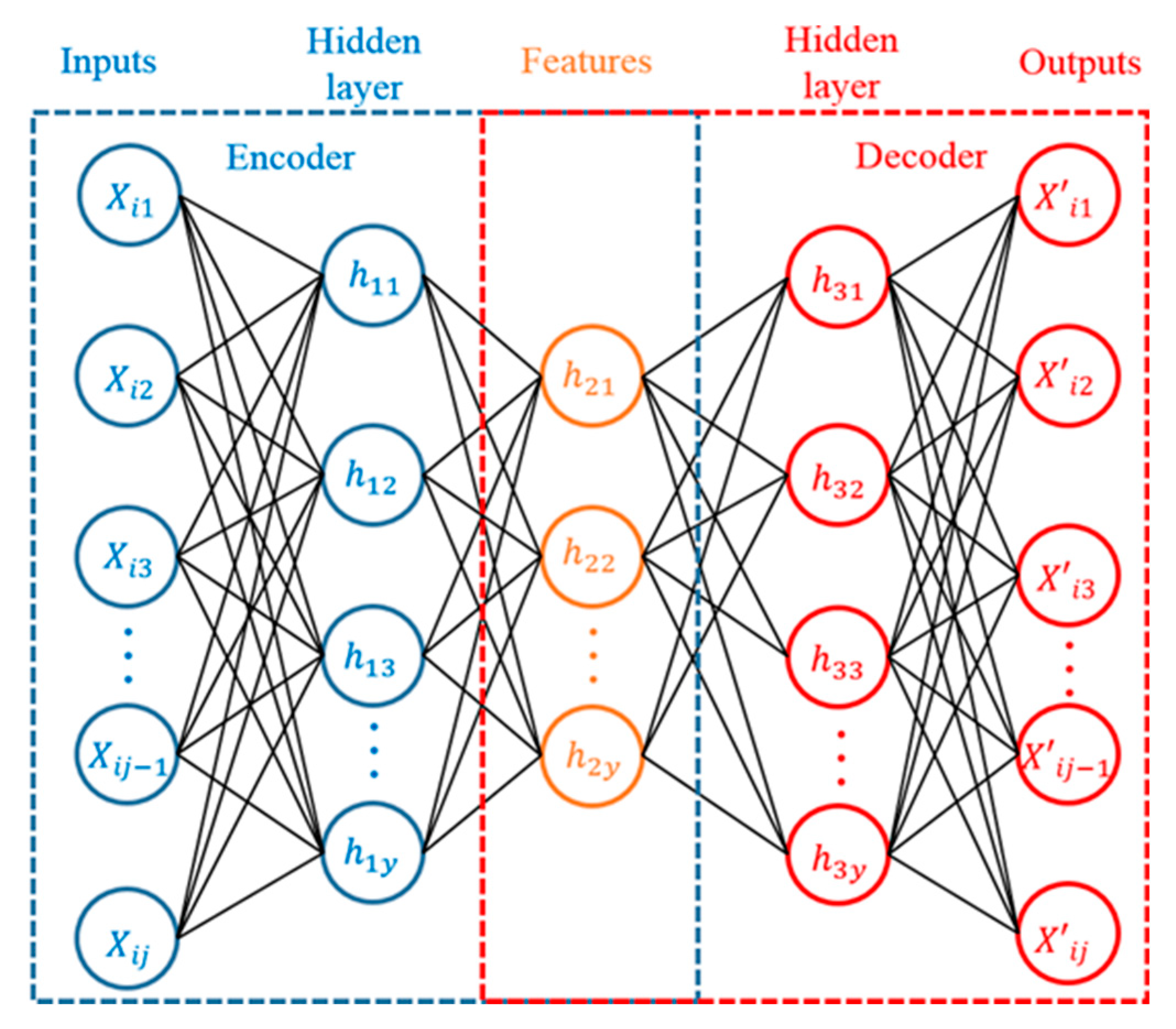
AE is used to reduce the data dimension and achieve the effect of feature extraction. As shown in Figure 4, the encoder will reduce the dimension of the data and transform the original data into a new space. The features in this space can describe the data more concisely than the original features. The orange neurons in the middle of the Figure are the features in the new space. The feature value is obtained by multiplying the weight matrix of the neurons in the hidden layer of the previous layer and adding the error vector (Equation (16)), where f() is the activation function which is Relu in this model, W is the weight matrix, $h_l$ is the error vector, b is the bias.

$$Features:f\left(\mathit{W}*h_l\right)+b$$

(16)

The data collected by sensors is a series of continuous data. However, in the general model, it only uses the current sensor value to predict the RUL. The change in historical sensor value is not considered. In this study, a new data processing method is proposed to take historical information into account. The format of the data will be converted from the original two-dimensional (samples, features) to three-dimensional (samples, time steps, features). Zero-padding is often used in signal processing or Convolutional Neural Networks (CNN). The purpose is to keep or increase the dimension of the data without affecting the information of the data itself. In this study, when the current sensor record has no historical data, the zero-padding method will be used to keep the data dimension.

3.1.2. Maximum RUL Transformation

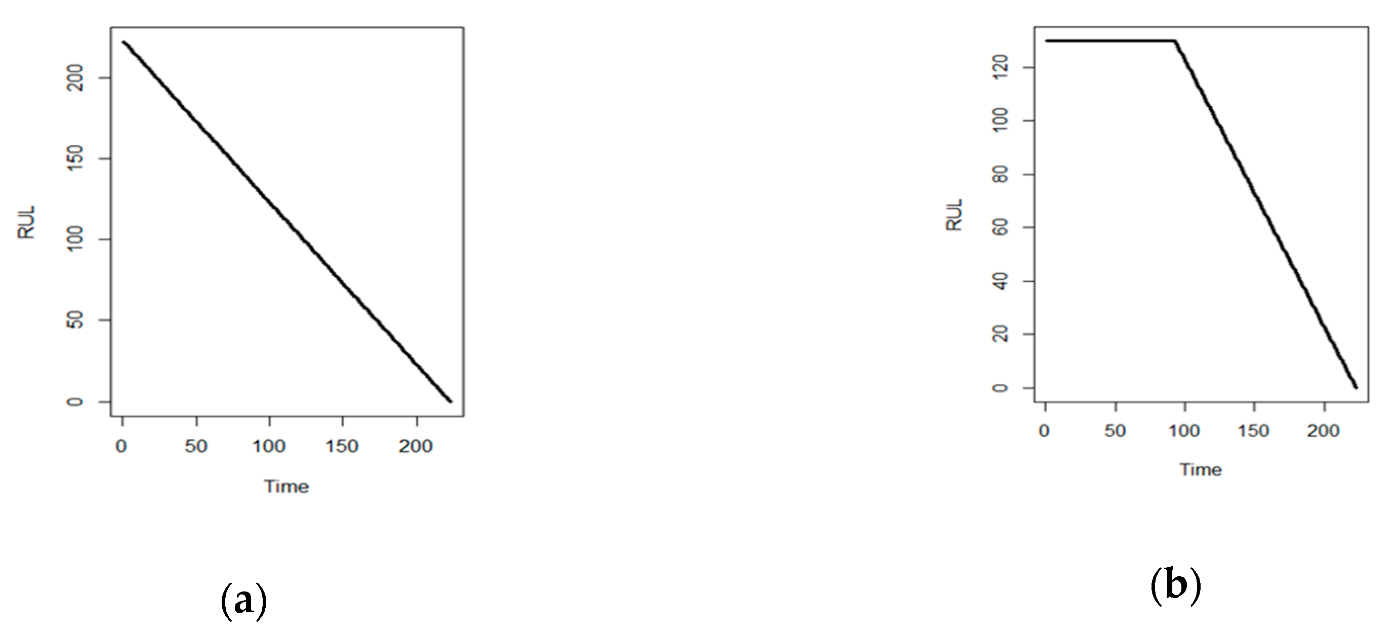
The maximum and minimum life of the engine is 356 and 127 cycles, and the average engine life is 209. The literature related to the prediction of RUL converts the maximum RUL to a specific reasonable value in the experiment. In this study, the transform process refers to the setting of T = 130 in Heimes [3]. The RUL greater than T will be defined as T, the RUL less than T will not change (Equation (17)). Figure 5 shows the life transform of one of the engines in the data set. Through this conversion, the RUL changes from the original linear decline to a nonlinear decline. Both the model training and the estimation of the RUL have better results in the setting.

$$RU{L}^{’}=\{\begin{array}{c}T,ifRUL\ge T\\ RUL,ifRUL<T\end{array}$$

(17)

3.2. RUL Prediction Model

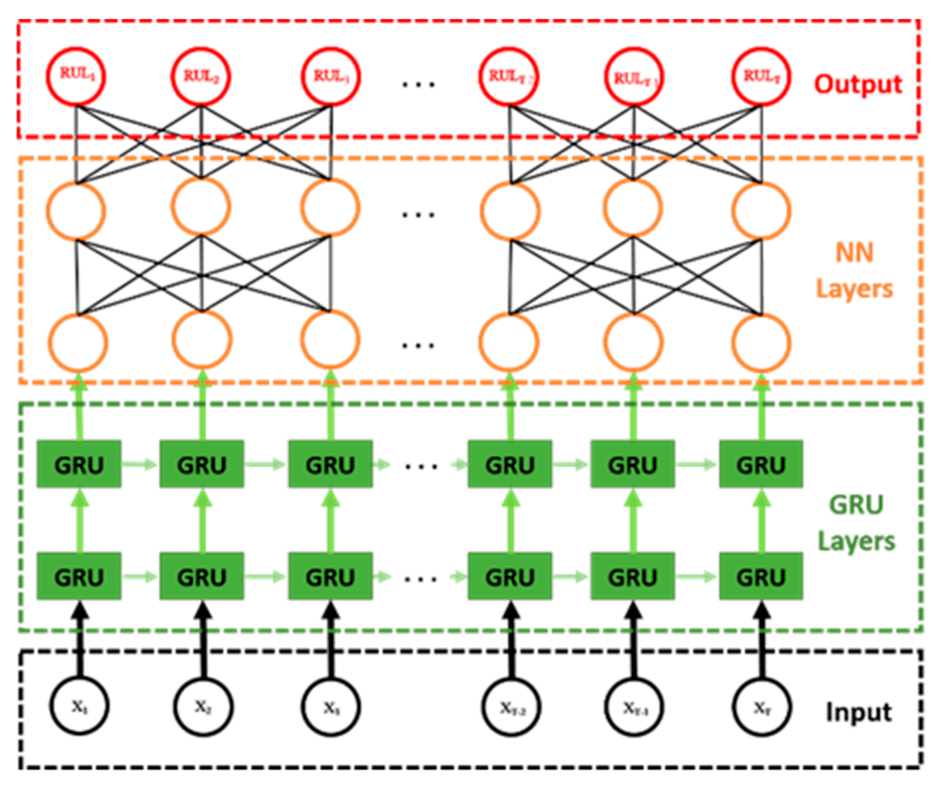
The RUL prediction model of this study combines the advantages of effective feature extraction and fast calculation. The RUL prediction model will be divided into four steps as shown in Figure 6. Step 1 is the input layer. $X_t$ represents the sensor data collected at the current time, $X_{t-1}$ represents the sensor data collected at the previous moment, $X_{t-2}$ represents the sensor data collected two moments earlier. The number of historical time points of sensor data to input to the model are adjustable. Step 2 is the GRU layer. The number of GRU layers is set to two in this paper. The number of GRU neurons will be tuned in the experimental part, and the best parameter combination selected for the research. The purpose of this step is to identify time series correlation in the input data through GRU. However, GRU cannot directly predict the RUL. Therefore, DNN must be added to predict the RUL. Step 3 is the DNN layer. DNN will convert the features extracted by GRU to the prediction dimension to perform the prediction. The best parameter combination from the experiment result will be used to decide the number of neurons as in Step 2. The objective function of DNN is applied to calculate the difference between the predicted value and the true value. In this study, Mean Square Error (MSE) is used as the objective function (Equation (18)), and the gradient descent method is used to minimize the objective function and train the model. Step 4 is the output layer of the model. The output is the value of predicted RUL at the current time. The model evaluation is conducted by calculating Root Mean Square Error (RMSE).

$$MSE=\frac{1}{n}{\displaystyle \sum }_{i=1}^n{\left(y_i-{y^{\prime }}_i\right)}^2$$

(18)

4. Result Evaluation

4.1. Data Collection

To validate the proposed AE-GRU, a Turbofan Engine Degradation Simulation Data Set (Prognostics and Management 2008, PHM08) (https://www.nasa.gov/) is used for performance evaluation in this section. It was carried out by a NASA tool C-MAPSS, to simulate the real large commercial aircraft turbofan engines. The data consists of a lot of time series cycles, which come from different engines of the same type. Each engine starts with a different wear level. The first section introduces the engine data collected by the sensor, and the second section describes the parameter settings of the model. The performance of different activation functions is compared and performance is optimized. Finally, the number of hidden layers and neurons is compared. In the third section, we will extract the best parameters and apply them to different models, and test the model by analyzing the root mean square error (RMSE).

There are data for 218 turbo engines, and a total of 45,918 records in the dataset. Every record has 26 original features and the customized RUL. The experimental design and verification of this study adopts k-fold cross validation to ensure the stability of the model.

Figure 7 is a diagram of the sensor parameters of the turbine engines in this study. The sensor parameters of Engine 1 are presented visually. The parameter values of the sensors vary in range and the parameter trends are not consistent. The RUL of the engine will be predicted by the changes of these sensor parameters in this research.

4.2. Hyperparameters Setting

Based on the experience of adjusting the model, the hyperparameters in the neural network will significantly affect the results of the model. This section finds the best parameter combination to apply in the model to predict the RUL value.

In experiments on neural networks, the number of hidden layers and the number of neurons are often the most difficult to choose. The training results will also depend on the quality of batch size and epoch. Batch size means the number of samples to work through in one iteration. Epoch is the number of times that the model goes through batches to go through the entire training dataset once. For example, if a training dataset has 3000 records and batch size is set to 500, it takes 6 iterations to complete an epoch.

4.2.1. Activation Function

The main function of the activation function in the neural network is to introduce nonlinear characteristics. If there is no activation function in the neural network, the input and output will only correlate with a simple linear relationship and not able to handle complex issues, so the activation function is very important in deep learning.

This experiment sets the following parameters to observe the training result of the GRU model with different activation functions:

• Epochs: 100;
• Optimizers: Adam;
• Batch_size: 128;
• Hidden layer, number of neurons: 1, 50;
• Inputs: 24.

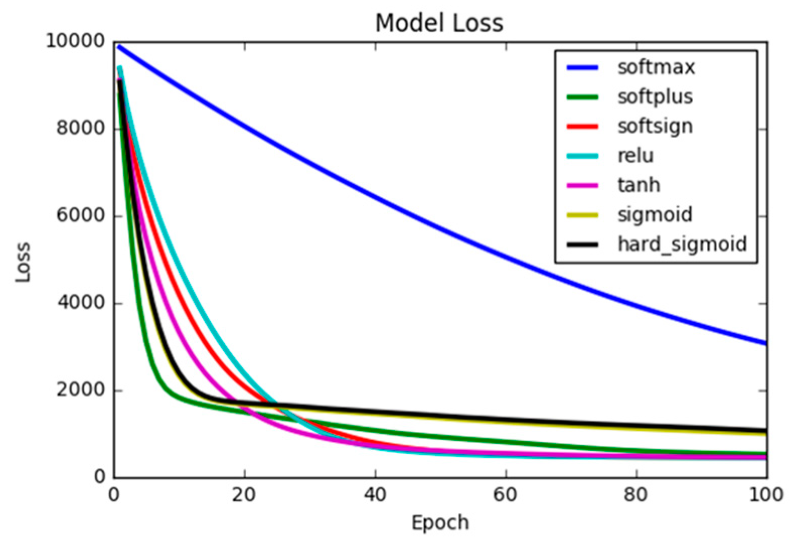
This experiment uses a 5-fold cross-validation to compare total seven activation functions and calculate the average loss of each activation function: softmax (3055.5), softplus (517.0), softsign (438.9), relu (434.8), tanh (445.3), sigmoid (990.7), hard sigmoid (1051.9). According to the training results, we find that the softmax performance is relatively poor, and the relu activation function performs best (Figure 8). The softmax activation function is a blend of multiple sigmoid, which is relatively suited to multiclass classification problems rather than a regression problem. The advantage of the Relu activation function is that neuron deactivation will only happen when the output of linear transformation is zero. The neurons will not be activated at the same time, but a certain number of neurons will be activated at a time. The objective function of Relu can be express as [41]:

$$f\left(x\right)=\max \left(0,x\right)$$

(19)

In addition, since the relu activation function does not need to perform exponential calculations, the convergence speed is fast and the calculation complexity levels are low. So, this study adopted relu as the activation function.

4.2.2. Optimizer

The purpose of optimizers is to minimize the loss function and the gap between the predicted value and real value. This experiment sets the following parameters and observes the training result of the GRU model under different optimizers:

• Epochs: 100;
• Activation: relu;
• Batch_size: 128;
• Hidden layer, number of neuron: 1, 50;
• Inputs: 24.

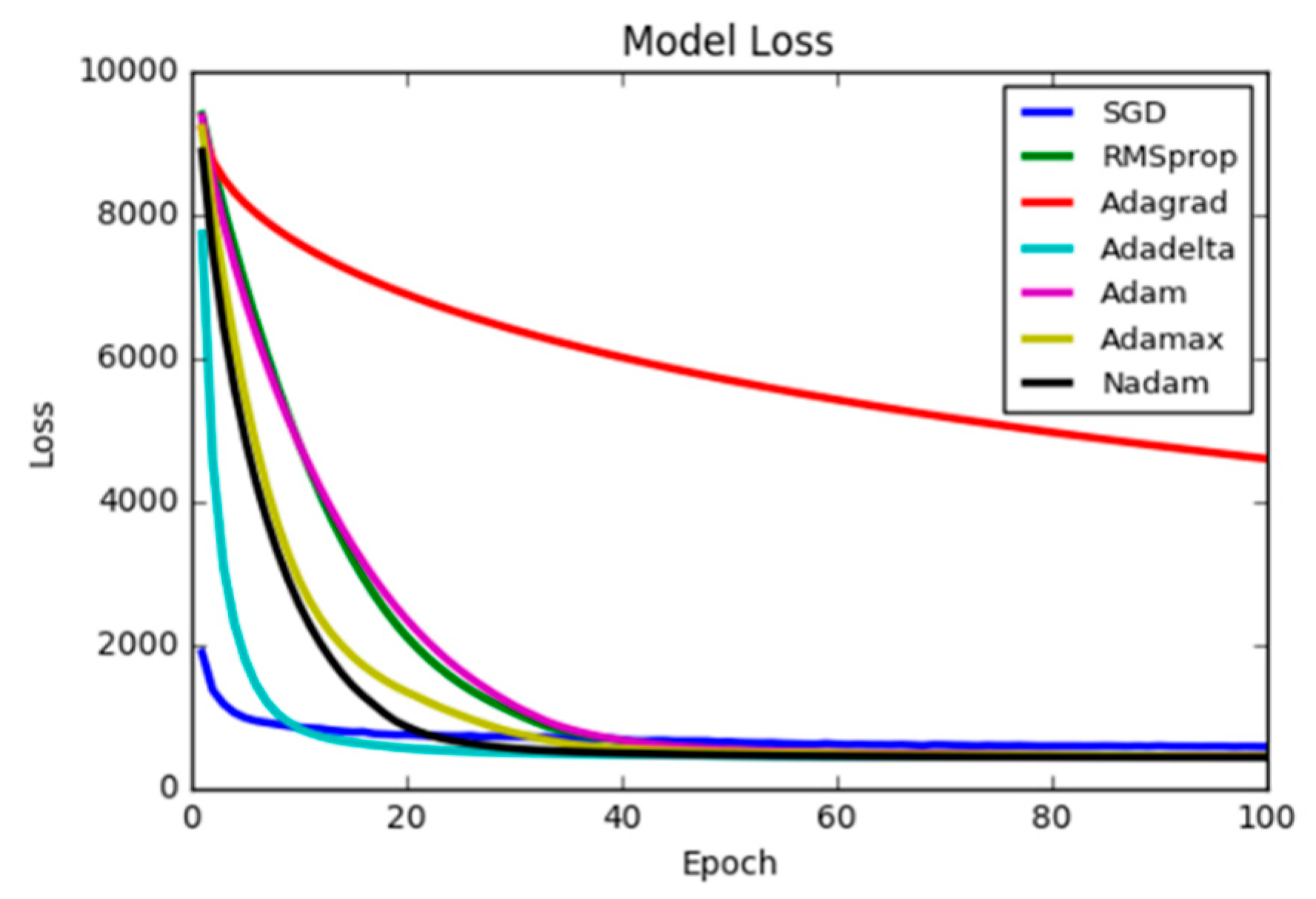
This experiment applies 5-fold cross-validation to compare a total of seven optimization algorithms: SGD (569.8), RMSprop (438.7), Adagrad (4586.9), Adadelta (426.6), Adam (436.6), Adamax (436.8), Nadam (420.7). The parameter setting of each optimization algorithm is the best result proposed in the literature. Kingma and Ba [42] proposed Adam’s optimization algorithm. Most of the current neural networks apply Adam to optimize the loss function. The advantage of Adam is quick convergence and dealing with high noise and the problem of sparse gradients. The Nadam optimization algorithm proposed by Dozat [43] changes the part of Adam’s momentum and accelerates the convergence rate of the model. The study confirms that in this PHM08 dataset, Nadam will converge faster than Adam (Figure 9). Therefore, the optimizer used in this study is Nadam.

4.2.3. Number of Hidden Layers and Neurons

This experiment compares three different batch sizes: 32 (

Table 2. Comparison of Root Mean Square Error (RMSE) result (batch size = 32).

Networks	Epochs	Training Time	RMSE
G(32,32)N(8,8)	33	98.4 s	20.18
G(64,64)N(8,8)	20	89.3 s	20.24
G(32,64)N(8,8)	19	76.8 s	20.37
G(32,64)N(16,16)	28	103.7 s	20.24
G(96,96)N(8,8)	25	150.3 s	20.20
G(96,96)N(16,16)	24	151.4 s	20.18

), 64 (

Table 3. Comparison of RMSE result (batch size = 64).

Networks	Epochs	Training Time	RMSE
G(32,32)N(8,8)	21	52.0 s	20.32
G(64,64)N(8,8)	24	75.8 s	20.25
G(32,64)N(8,8)	23	63.8 s	20.33
G(32,64)N(16,16)	24	66.7 s	20.36
G(96,96)N(8,8)	15	80.1 s	20.44
G(96,96)N(16,16)	14	78.3 s	20.44

), 128 (

Table 4. Comparison of RMSE result (batch size = 128).

Networks	Epochs	Training Time	RMSE
G(32,32)N(8,8)	42	60.4 s	20.16
G(64,64)N(8,8)	34	70.1 s	20.07*
G(32,64)N(8,8)	33	60.3 s	20.20
G(32,64)N(16,16)	52	85.6 s	20.19
G(96,96)N(8,8)	42	119.4 s	20.15
G(96,96)N(16,16)	36	115.7 s	20.12

). The early stopping function has been adopted in the experiment; if the MSE of verification does not rise for 10 consecutive times, the training will stop and the previous best model will be used in the test dataset. Early stopping is commonly used in the algorithm of gradient descent to avoid overfitting. The GRU and DNN layers are set to two layers. The RMSE result of different neurons in the training are compared. The input of this experiment is 24 parameters of the current raw data of the sensor, and there is no historical information (time steps = 1).

The experimental results show that the larger the batch size, the faster the model training speed. Therefore, batch size in this study will be set to 128. When the batch size is greater, not only the training time is fast, but the RMSE results are also better. So, the network architecture of this study will be set to G(64,64)N(8,8).

4.3. Model Evaluation

4.3.1. Model Comparison

This section uses the 5-fold cross-validation to evaluate the validity of the RUL model of the AE-GRU in this study, and compares the results of existing models. In total 218 engines are divided into five parts as 44, 44, 44, 44 and 42 engines. Four parts are used for training each time, and the remainder are test data. After distinguishing the data, the AE model reduces the dimension of the data, and then predicts the RUL of the engine through GRU. The performance of the model is also compared using the RMSE result. The dimension of the data is reduced from 24 inputs of the original data to 15, 10, 5. AE extracts the characteristics of the original data by non-linear transformation, and through multiple hidden layers, observing the loss of each feature in the compression and restoration process (

Table 5. Loss of dimension reduction by AE.

Input	15	10	5
Loss	7.7 × 10−6	2.6 × 10−5	3.0 × 10−5

).

The experimental results show that the dimension reduction effect is the best when the input is reduced to 15 dimensions. In 10 or 5 dimensions, the effect of restoration is poor because of the loss of original data Information. In this study, the AE will reduce the data dimension from 24 to 15 and compare the performance with other models.

After 5-fold cross-validation, (

Table 6. RMSE results of different models under 5-fold cross-validation (Time steps = 5).

	DNN Inputs:24	RNN Inputs:24	LSTM Inputs:24	GRU Inputs:24	AE-GRE Inputs:15
1	18.57	18.06	17.80	17.68	17.64
2	18.76	18.22	18.00	17.88	17.70
3	18.73	18.47	18.19	18.03	17.98
4	19.11	18.44	18.45	18.16	18.20
5	19.12	18.43	18.34	18.12	18.20
Average	18.86	18.32	18.16	17.96	17.94

and

Table 7. RMSE results of different models under 5-fold cross-validation (Time steps = 10).

	DNN Inputs:24	RNN Inputs:24	LSTM Inputs:24	GRU Inputs:24	AE-GRE Inputs:15
1	19.21	15.08	11.20	10.31	10.39
2	19.21	14.26	11.52	11.05	10.02
3	19.07	15.86	10.78	10.75	10.70
4	19.77	15.07	11.49	11.33	10.69
5	19.69	17.27	10.81	10.54	11.31
Average	19.39	15.51	11.16	10.79	10.62

), it is found that when the input of AE-GRU is reduced from the original 24 features to 15, the RMSE results are better than those of other models. This confirms that AE-GRU can effectively extract features and accurately predict the RUL. Time steps is the number of historical data points. time steps = 5 is the historical information of the current time point and the previous four-time records. time steps = 10 is the current time information and the previous nine-time points. The results show that when time steps = 5, the results of the model are quite close. When time steps = 10, because of the large amount of historical data, the RNN has the problem of disappearing gradients, while the general DNN has no time series characteristics, and the prediction results are the worst.

4.3.2. RUL Prediction

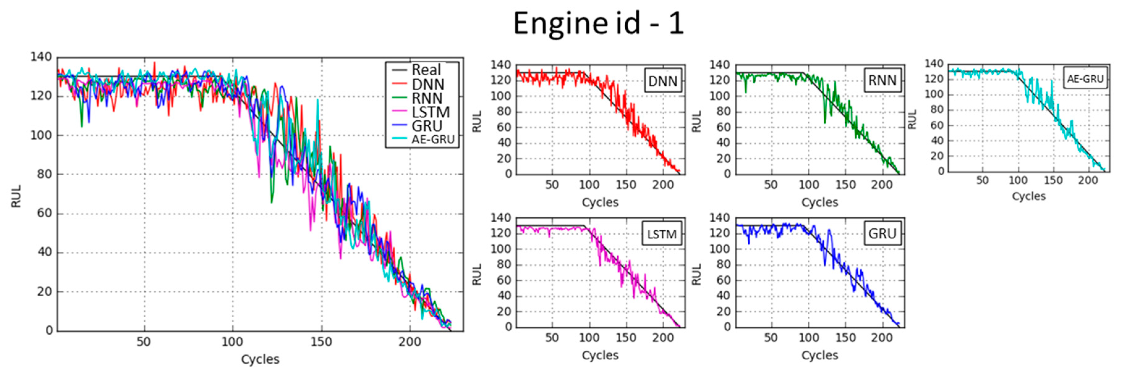
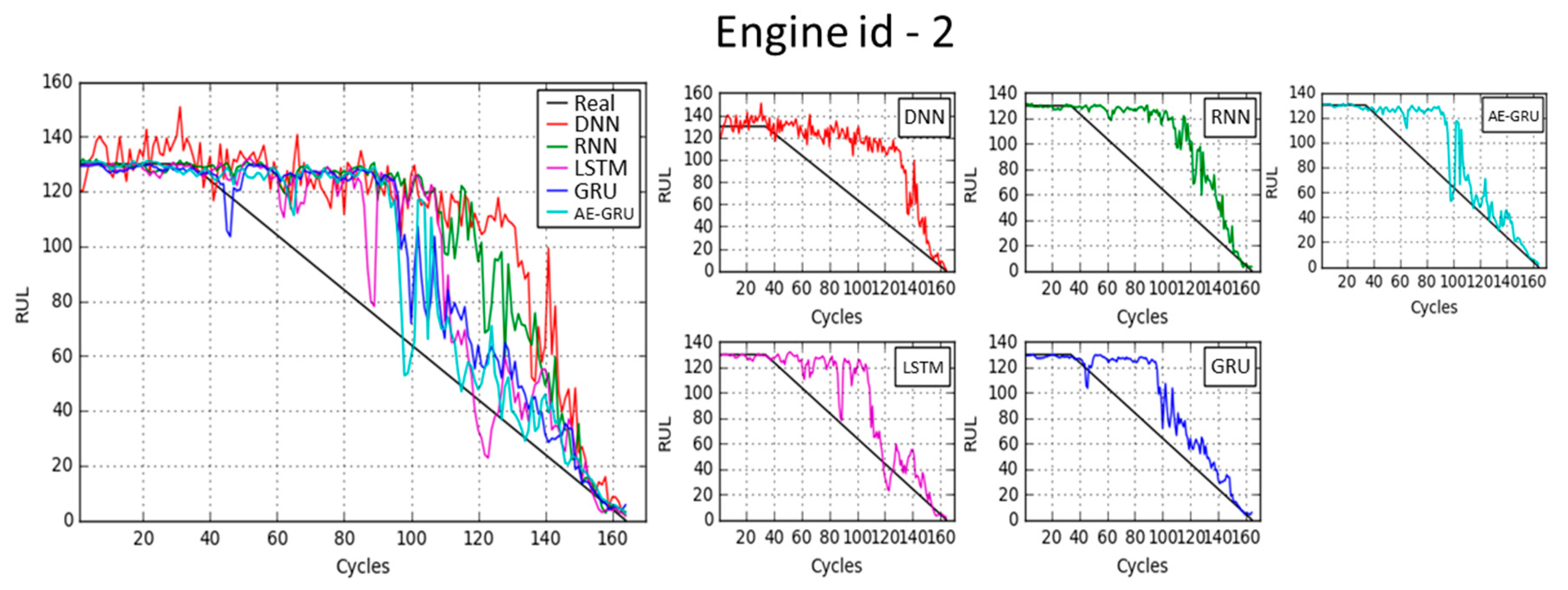
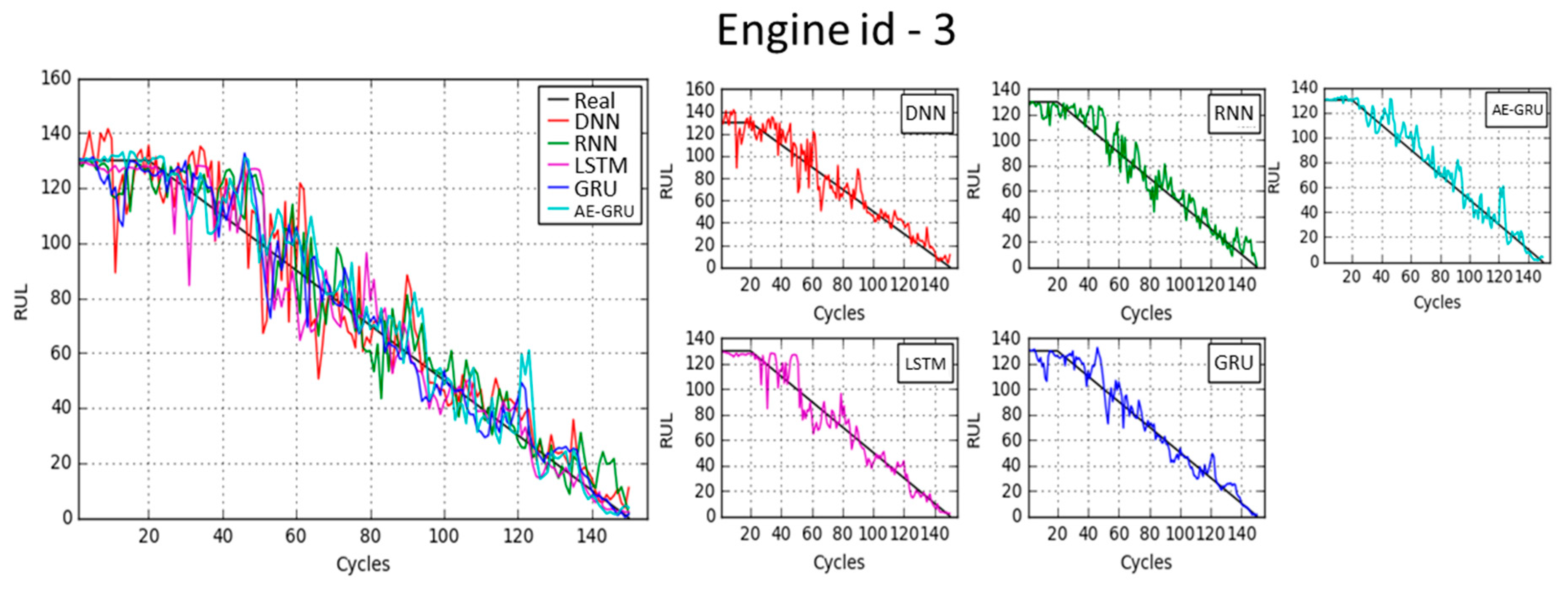
Figure 10, Figure 11 and Figure 12 show the test results for the total of five model methods (DNN, RNN, LSTM, GRU, and AE-GRU). According to the Figure, it can be seen that the five models have the problem of unstable fluctuation. Neither DNN nor RNN are ideal for training or testing. LSTM, GRU and AE-GRU are good in the training set, but precarious in the testing set, because there is not enough training data. Deep learning requires a large amount of data identify features. When the RUL is stable for 130 cycles, the AE-GRU proposed in this study can have more accurate results in predicting the RUL of the engine. It will not fluctuate like DNN and RNN. When the RUL begins to decline, AE-GRU can predict it in advance.

5. Conclusions

This study proposes the AE-GRU model for RUL prediction. First, pre-processing was applied to the sensor data collected by different sensors. Because the scales of different sensors are not the same, we standardize the sensor data so that the sensor data can be rearranged to the same scale standard while retaining the characteristics of the data time series. Next, the RUL is defined. The purpose of defining the RUL is to allow the user to accurately predict the life value of equipment that the engine can work. Feature extraction finds the characteristics of the sensor data by deep learning. The characteristics will directly affect the predictive ability of the model. A good model is indispensable for characteristics that can fully represent the data. Data dimension conversion takes the historical sensor data into account, because the data has the characteristics of a time series. The last step of data pre-processing is the transformation of the maximum life value. The engine with an RUL greater than 130 cycles is set to 130 cycles. When using the RUL prediction, attention focuses on the RUL value when it is about to break, and the situation where the RUL value is still very large is less important. Then the GRU is combined with the back-propagation algorithm to learn the parameters. Because there are a large number of parameters to learn, the experiment uses a GPU graphics card in parallel operation and increase the process speed. At the same time, the relu activation function and Nadam optimizer are used to make the process of learning parameters converge more quickly. Combined with the best combination of parameters run under the experimental design, the prediction of the RUL has better results.

The contribution of this study is that it applies the optimized version of LSTM, the GRU. GRU can effectively capture the characteristics of the sensor data, and extract the characteristics of the data by AE before the RUL model prediction. The GRU model has many fewer parameters than LSTM but still retains the advantages of LSTM. The AE-GRU model proposed in this study has a shorter training time, and also takes advantage of the features extracted by AE. The convergence speed of the model is much faster. The validity of the model is evaluated and verified through the 5-fold cross-validation. The results of the root mean square error are better than other deep learning methods, and the research model can find the engine that is about to fail early and in time to maintain the equipment, reducing unnecessary costs.

The AE-GRU model proposed in this study has good accuracy in the prediction of RUL. With the improvement of process technology, the cost of equipment will become higher and higher. Therefore, more complex models may be needed in future research, such as a bi-directional recurrent network. In this study, only a directional recurrent network is considered. In some cases, the output at the current moment is not only related to the previous state, but also closely related to the state after it.

The pre-processing method in this study extracts features from the original data. Although the features can effectively represent the data set, they may contain a little noise. In the future, the pre-processing method might also employ an advanced version of AE, such as denoising AE (DAE). The combination of these two methods can further improve the prediction of RUL.

If the algorithm can be effectively implemented, predictive maintenance can be widely used in many applications, providing effective information for early maintenance of machinery, and self-correcting parameters can improve the yield to achieve the target of smart factories.

References

1. Wang, S.; Wan, J.; Li, D.; Zhang, C. Implementing Smart Factory of Industrie 4.0: An Outlook. Int. J. Distrib. Sens. Netw. 2016, 12, 3159805. [Google Scholar] [CrossRef] [Green Version]
2. Chien, C.-F.; Hsu, C.-Y.; Chen, P.-N. Semiconductor Fault Detection and Classification for Yield Enhancement and Manufacturing Intelligence. Flex. Serv. Manuf. J. 2013, 25, 367–388. [Google Scholar] [CrossRef]
3. Hsu, C.-Y.; Liu, W.-C. Multiple Time-Series Convolutional Neural Network for Fault Detection and Diagnosis and Empirical Study in Semiconductor Manufacturing. J. Intell. Manuf. 2020, 1–14. [Google Scholar] [CrossRef]
4. Fan, S.-K.S.; Hsu, C.-Y.; Tsai, D.-M.; He, F.; Cheng, C.-C. Data-Driven Approach for Fault Detection and Diagnostic in Semiconductor Manufacturing. IEEE Trans. Autom. Sci. Eng. 2020, 1–12. [Google Scholar] [CrossRef]
5. Shrouf, F.; Ordieres, J.; Miragliotta, G. Smart factories in Industry 4.0: A review of the concept and of energy management approached in production based on the Internet of Things paradigm. In Proceedings of the 2014 IEEE International Conference on Industrial Engineering and Engineering Management, Selangor, Malaysia, 9–12 December 2014; pp. 697–701. [Google Scholar]
6. Kothamasu, R.; Huang, S.H.; VerDuin, W.H. System health monitoring and prognostics—A review of current paradigms and practices. Int. J. Adv. Manuf. Technol. 2006, 28, 1012–1024. [Google Scholar] [CrossRef]
7. Peng, Y.; Dong, M.; Zuo, M.J. Current status of machine prognostics in condition-based maintenance: A review. Int. J. Adv. Manuf. Technol. 2010, 50, 297–313. [Google Scholar] [CrossRef]
8. Soh, S.S.; Radzi, N.H.; Haron, H. Review on scheduling techniques of preventive maintenance activities of railway. In Proceedings of the 2012 Fourth International Conference on Computational Intelligence, Modelling and Simulation, Kuantan, Malaysia, 25–27 September 2012; pp. 310–315. [Google Scholar]
9. Heimes, F.O. Recurrent neural networks for remaining useful life estimation. In Proceedings of the 2008 International Conference on Prognostics and Health Management, Denver, CO, USA, 6–9 October 2008; pp. 1–6. [Google Scholar]
10. Li, Y.; Shi, J.; Gong, W.; Liu, X. A data-driven prognostics approach for RUL based on principle component and instance learning. In Proceedings of the 2016 IEEE International Conference on Prognostics and Health Management (ICPHM), Ottawa, ON, Canada, 20–22 June 2016; pp. 1–7. [Google Scholar]
11. Murphy, K.P. Machine Learning: A Probabilistic Perspective; MIT Press: Cambridge, MA, USA, 2012. [Google Scholar]
12. Cortes, C.; Vapnik, V. Support-Vector Networks. Mach. Learn. 1995, 20, 273–297. [Google Scholar] [CrossRef]
13. Breiman, L. Random forests. Mach. Learn. 2001, 45, 5–32. [Google Scholar] [CrossRef] [Green Version]
14. Chen, T.; Guestrin, C. XGBoost: A Scalable Tree Boosting System. In Proceedings of the 22nd ACM SIGKDD International Conference on Knowledge Discovery and Data Mining, San Francisco, CA, USA, 13–17 August 2016; ACM: New York, NY, USA, 2016. [Google Scholar]
15. Han, Z.; Zhao, J.; Leung, H.; Ma, K.F.; Wang, W. A review of deep learning models for time series prediction. IEEE Sens. J. 2019. [Google Scholar] [CrossRef]
16. Bengio, Y.; Courville, A.; Vincent, P. Representation Learning: A Review and New Perspectives. IEEE Trans. Pattern Anal. Mach. Intell. 2013, 35, 1798–1828. [Google Scholar] [CrossRef]
17. Schmidhuber, J. Deep Learning in Neural Networks: An Overview. Neural Netw. 2015, 61, 85–117. [Google Scholar] [CrossRef] [Green Version]
18. LeCun, Y.; Bengio, Y.; Hinton, G. Deep learning. Nature 2015, 521, 436–444. [Google Scholar] [CrossRef] [PubMed]
19. Makridakis, S.; Spiliotis, E.; Assimakopoulos, V. Statistical and Machine Learning Forecasting Methods: Concerns and Ways Forward. PLoS ONE 2018, 13, e0194889. [Google Scholar] [CrossRef] [PubMed] [Green Version]
20. Alfred, R.; Obit, J.H.; Ahmad Hijazi, M.H.; Ag Ibrahim, A.A. A performance comparison of statistical and machine learning techniques in learning time series data. Adv. Sci. Lett. 2015, 21, 3037–3041. [Google Scholar]
21. Hinton, G.E.; Salakhutdinov, R.R. Reducing the dimensionality of data with neural networks. Science 2006, 313, 504–507. [Google Scholar] [CrossRef] [Green Version]
22. Lin, P.; Tao, J. A Novel Bearing Health Indicator Construction Method Based on Ensemble Stacked Autoencoder. In Proceedings of the 2019 IEEE International Conference on Prognostics and Health Management (ICPHM), San Francisco, CA, USA, 17–20 June 2019; pp. 1–9. [Google Scholar]
23. Yin, C.; Zhang, S.; Wang, J.; Xiong, N.N. Anomaly Detection Based on Convolutional Recurrent Autoencoder for IoT Time Series. IEEE Trans. Syst. Man Cybern. Syst 2020, 1–11. [Google Scholar] [CrossRef]
24. Hochreiter, S.; Schmidhuber, J. Long short-term memory. Neural Comput. 1997, 9, 1735–1780. [Google Scholar] [CrossRef]
25. Zhang, Y.; Xiong, R.; He, H.; Liu, Z. A LSTM-RNN method for the lithuim-ion battery remaining useful life prediction. In Proceedings of the 2017 Prognostics and System Health Management Conference (PHM-Harbin), Harbin, China, 9–12 July 2017; pp. 1–4. [Google Scholar]
26. Mathew, V.; Toby, T.; Singh, V.; Rao, B.M.; Kumar, M.G. Prediction of Remaining Useful Lifetime (RUL) of turbofan engine using machine learning. In Proceedings of the 2017 IEEE International Conference on Circuits and Systems (ICCS), Batumi, Georgia, 5–8 December 2017; pp. 306–311. [Google Scholar]
27. Zheng, S.; Ristovski, K.; Farahat, A.; Gupta, C. Long short-term memory network for remaining useful life estimation. In Proceedings of the 2017 IEEE international conference on prognostics and health management (ICPHM), Dallas, TX, USA, 19–21 June 2017; pp. 88–95. [Google Scholar]
28. Chen, J.; Jing, H.; Chang, Y.; Liu, Q. Gated recurrent unit based recurrent neural network for remaining useful life prediction of nonlinear deterioration process. Reliab. Eng. Syst. Safe. 2019, 185, 372–382. [Google Scholar] [CrossRef]
29. Cho, K.; Van Merriënboer, B.; Gulcehre, C.; Bahdanau, D.; Bougares, F.; Schwenk, H.; Bengio, Y. Learning phrase representations using RNN encoder-decoder for statistical machine translation. arXiv 2014, arXiv:1406.1078. [Google Scholar]
30. Chung, J.; Gulcehre, C.; Cho, K.; Bengio, Y. Empirical evaluation of gated recurrent neural networks on sequence modeling. arXiv 2014, arXiv:1412.3555. [Google Scholar]
31. Chen, Z.; Liu, Y.; Liu, S. Mechanical state prediction based on LSTM neural netwok. In Proceedings of the 2017 36th Chinese Control Conference (CCC), Dalian, China, 26–28 July 2017; pp. 3876–3881. [Google Scholar]
32. Zheng, J.; Xu, C.; Zhang, Z.; Li, X. Electric load forecasting in smart grids using long-short-term-memory based recurrent neural network. In Proceedings of the 2017 51st Annual Conference on Information Sciences and Systems (CISS), Baltimore, MD, USA, 22–24 March 2017; pp. 1–6. [Google Scholar]
33. ElSaid, A.; Wild, B.; Higgins, J.; Desell, T. Using LSTM recurrent neural networks to predict excess vibration events in aircraft engines. In Proceedings of the 2016 IEEE 12th International Conference on e-Science, Baltimore, MD, USA, 23–27 October 2016; pp. 260–269. [Google Scholar]
34. Cenggoro, T.W.; Siahaan, I. Dynamic bandwidth management based on traffic prediction using Deep Long Short Term Memory. In Proceedings of the 2016 2nd International Conference on Science in Information Technology (ICSITech), Balikpapan, Indonesia, 26–27 October 2016; pp. 318–323. [Google Scholar]
35. Bao, W.; Yue, J.; Rao, Y. A deep learning framework for financial time series using stacked autoencoders and long-short term memory. PLoS ONE 2017, 12, e0180944. [Google Scholar] [CrossRef] [Green Version]
36. Zhang, Q.; Wang, H.; Dong, J.; Zhong, G.; Sun, X.J.I.G.; Letters, R.S. Prediction of sea surface temperature using long short-term memory. IEEE Geosci. Remote Sens. Lett. 2017, 14, 1745–1749. [Google Scholar] [CrossRef] [Green Version]
37. How, D.N.T.; Sahari, K.S.M.; Yuhuang, H.; Kiong, L.C. Multiple sequence behavior recognition on humanoid robot using long short-term memory (LSTM). In Proceedings of the 2014 IEEE international symposium on robotics and manufacturing automation (ROMA), Kuala Lumpur, Malaysia, 15–16 December 2014; pp. 109–114. [Google Scholar]
38. Truong, A.M.; Yoshitaka, A. Structured LSTM for human-object interaction detection and anticipation. In Proceedings of the 2017 14th IEEE International Conference on Advanced Video and Signal Based Surveillance (AVSS), Lecce, Italy, 29 August–1 September 2017; pp. 1–6. [Google Scholar]
39. Kuan, L.; Yan, Z.; Xin, W.; Yan, C.; Xiangkun, P.; Wenxue, S.; Zhe, J.; Yong, Z.; Nan, X.; Xin, Z. Short-term electricity load forecasting method based on multilayered self-normalizing GRU network. In Proceedings of the 2017 IEEE Conference on Energy Internet and Energy System Integration (EI2), Beijing, China, 26–28 November 2017; pp. 1–5. [Google Scholar]
40. Zhang, D.; Kabuka, M.R. Combining weather condition data to predict traffic flow: A GRU-based deep learning approach. IET Intell. Transp. Syst. 2018, 12, 578–585. [Google Scholar] [CrossRef]
41. Sharma, S. Activation functions in neural networks. Int. J. Eng. Appl. Sci. Technol. 2020, 4, 310–316. [Google Scholar] [CrossRef]
42. Kingma, D.P.; Ba, J. Adam: A method for stochastic optimization. arXiv 2014, arXiv:1412.6980. [Google Scholar]
43. Dozat, T. Incorporating nesterov momentum into adam. In Proceedings of the 2016 International Conference on Learning Representations (ICLR), San Juan, Puerto Rico, 2–4 May 2016; pp. 1–4. [Google Scholar]
Figure 1. Structure of Long Short-Term Memory (LSTM) unit.
Processes 08 01155 g001
Figure 2. Structure of gated recurrent neural network.
Processes 08 01155 g002
Figure 3. Research framework of Autoencoder Gated Recurrent Unit (AE-GRU).
Processes 08 01155 g003
Figure 4. AE Structure
Processes 08 01155 g004
Figure 5. Maximum life value transform (a) original RUL; (b) RUL after Maximum useful life transform.
Processes 08 01155 g005
Figure 6. Model structure of AE-GRU for RUL prediction.
Processes 08 01155 g006
Figure 7. Diagram of turbine engine sensor parameter.
Processes 08 01155 g007
Figure 8. Comparison of training result in different activation function
Processes 08 01155 g008
Figure 9. Comparison of training result in different optimizer.
Processes 08 01155 g009
Figure 10. Model testing results comparison (Engine 1).
Processes 08 01155 g010
Figure 11. Model testing results comparison (Engine 2).
Processes 08 01155 g011
Figure 12. Model testing results comparison (Engine 3).
Processes 08 01155 g012