On the Application of the FactSage Thermochemical Software and Databases in Materials Science and Pyrometallurgy

Abstract

The discovery of new metallic materials is of prime importance for the development of new technologies in many fields such as electronics, aerial and ground transportation as well as construction. These materials require metals which are obtained from various pyrometallurgical processes. Moreover, these materials need to be synthesized under extreme conditions of temperature where liquid solutions are produced and need to be contained. The design and optimization of all these pyrometallurgical processes is a key factor in this development. We present several examples in which computational thermochemistry is used to simulate complex pyrometallurgical processes including the Hall–Heroult process (Al production), the PTVI process (Ni production), and the steel deoxidation from an overall mass balance and energy balance perspective. We also show how computational thermochemistry can assist in the material selection in these extreme operation conditions to select refractory materials in contact with metallic melts. The FactSage thermochemical software and its specialized databases are used to perform these simulations which are proven here to match available data found in the literature.

1. Introduction

Computational thermochemistry is a powerful tool used by engineers and scientists as it allows the theoretical exploration of the energetic behavior of multicomponent and multiphasic systems for a wide range of conditions at a small computational cost. It can be used for example to predict the corrosion of a crucible by a chemically aggressive liquid metal, to identify the reaction products inside a primary metal smelter, to establish overall heat and mass balances of a process, and to generate phase mappings (such as phase diagrams and predominance diagrams).

Its algorithmic efficiency resides in (1) the use of simple and easily derivable mathematical functions to describe the energetic behavior of each phase, (2) the relatively small number of variables used to define the equilibrium state of the system, and (3) the need to respect thermodynamic constraints at equilibrium such as the Gibbs phase rule. The latter also greatly speeds up the calculations as it can be used to identify a good initial estimate of the equilibrium state of the system [1].

It is based on the identification of the equilibrium state of a system constrained by different conditions of temperature, pressure, volume, chemical potentials, chemical compositions, and more. The numerical algorithm used to identify complex equilibrium states needs to adequately converge toward the targeted local minimum associated with the initial phase assemblage estimate. This is a mathematical challenge as thermodynamic models of solutions often present multiple inflection points on their energetic surface and therefore have multiple local minima. Numerical strategies based on the Newton method (ex.: Lagrange-Sequential-Quadratic Newton method) are often used to solve such problems. Examples of efficient numerical methods available in the literature to solve these constrained minimization problems can be found in the work of Eriksson [2] and Harvey et al. [3]. After an equilibrium state candidate is identified, other constrained minimization problems need to be solved [3] to evaluate the activity of each potentially stable phase not considered in the phase assemblage. This step is of fundamental importance as it confirms that the global Gibbs free energy minimum for some imposed constraints has been reached. At this point, the computational time required to identify the equilibrium state exponentially grows as a function of the number of potentially stable phases considered in the calculations.

As will be shown in this work, computational thermochemistry is an essential and powerful tool in materials science and engineering that will always be required, even with the advent of ab initio methods, sophisticated atomistic Monte Carlo (MC) and Molecular Dynamics (MD) simulations as well as finite element algorithms. In fact, it is the only approach that allows the rapid identification and prediction of multicomponent and multiphasic equilibria. Ab initio methods are greatly limited in terms of the number of atoms that can be considered (i.e., the thousand atom scale) when describing a periodic structure. This is a consequence of the mathematical complexity required in evaluating the electronic behavior of the system (ex.: numerical resolution of the Schrodinger equation via density functional theory). With such a small number of considered atoms, it is definitively not possible to explore multiphasic equilibria. Atomistic simulations based on classical interatomic potentials can account for a substantially larger number of atoms. Because of this, classical MD simulations can be used to explore phase transitions such as melting and order-disorder solid–solid transitions. Moreover, more evolved methods such as the thermodynamic integration method can be implemented in atomistic simulations to directly access the Gibbs free energy of the considered atomic system. Even though it can consider large supercells, it is still not possible to represent important features of macroscopic phases with this approach such as grain size and grain boundaries. Finally, finite elements codes always require multiple thermodynamic data such as the phase assemblage and chemical potentials (and their derivatives) at every time step to be able to simulate the dynamic behavior of a system.

The quality and precision of the thermodynamic simulations depend on two important elements, i.e., the choice of a thermodynamic model to describe the energetics of a given phase and the optimal parameterization of these functions using experimental and numerical data. Since the appearance of a phase in a specific thermodynamic calculation is possible only if its Gibbs free energy function has been defined, it is of prime importance to review the literature to list all the important phases to be accounted for in subsequent calculations.

All of these strengths of computational thermochemistry are made available in the FactSage thermodynamic package [4]. This software is built on a robust and highly efficient Gibbs free energy minimization strategy that allows the calculations of phase equilibria and phase diagrams. This constrained minimization core has access to multiple specialized databases developed over the past 45 years. These databases can describe a multitude of multicomponent oxide, alloy, salt and aqueous systems. Moreover, these databases can be combined to describe a wide variety of multiphasic equilibria such as impurity partitioning in pyrometallurgical processes that involve the presence of a slag phase, impurity removal in metallic melts by salt fluxes and many other high temperature phase equilibria.

The aim of this work is to present essential concepts and practical applications of computational thermochemistry. Specific examples of its use in materials science and metallurgy are treated using the FactSage software. This paper is intended to serve as a reference for engineers and materials scientists who want to deepen their knowledge of computational thermochemistry and explore its various uses in research and development.

2. Fundamental Concepts of Computational Thermochemistry

2.1. Compounds vs. Solutions

The most critical aspect when evaluating the equilibrium state of a system is to consider all the phases that may potentially form. The phase selection prior to a calculation needs to be performed with great care. The omission of phases may impact drastically the identified equilibrium state. Two types of phases can form in a system: i.e., stoichiometric compounds and solutions.

A stoichiometric compound is a phase that can, to a good approximation, be represented by having a single chemical composition. It appears as a vertical line on conventional phase diagrams (ex.: Mg${}_2$SiO${}_4$ and MgSiO${}_3$ in Figure 1). These phases are typically forming in multicomponent systems that have a large and negative enthalpy of mixing. The strong heterogeneous chemical interactions stabilize these compounds.

The Gibbs energy function of a stoichiometric phase, i.e., $g^0\left(T,P_0\right)$, is defined as follows:

$$g^0\left(T,P_0\right)=h_{T_{ref}}^0+{\int }_{T_{ref}}^T{c}_P\mathrm{d}T-T\left[s_{T_{ref}}^0+{\int }_{T_{ref}}^T\frac{c_P}{T}\mathrm{d}T\right]$$

(1)

Equation (1) is built using three fundamental thermodynamic properties: the specific standard enthalpy of formation ($h_{T_{ref}}^0$), the specific isobaric heat capacity ($c_P$) and the specific standard entropy ($s_{T_{ref}}^0$). It is to be noted here that the absolute enthalpy of a system is not accessible in classical thermodynamics as nuclear and weak forces are not described. To overcome this limitation, we use reference states to express this quantity. Historically, the thermodynamic community has set the enthalpy of pure elements in their stable state at standard temperature and pressure conditions (298.15 K and 10${}^5$ Pa) to be equal to zero [5]. The specific standard entropy is evaluated by integrating the isobaric heat capacity from 0K to the reference temperature:

$$s_{T_{ref}}^0={\int }_0^{T_{ref}}\frac{c_P\left(T,P_0\right)}{T}dT$$

(2)

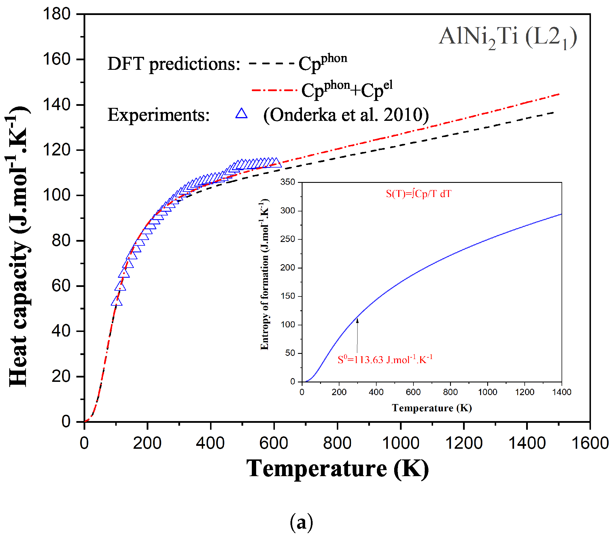
Equation (2) requires the measurement of the low temperature behavior of the isobaric heat capacity. For many stable and most metastable compounds, experimental heat capacity data are not available, especially in the low temperature range. Traditionally, the CALPHAD community used to estimate unknown $s^0$ (and heat capacities) using the Neumann–Kopp rule [6]. This rule simply assumes a linear behavior of the estimated thermodynamic property versus composition. For disordered solid solutions and molten phases, the Kopp–Neumann rule has been proven to be a good approximation in many cases. However, for stoichiometric compounds, it has severe limitations, mainly related to the difference in the electronic structure between the compound and its constituent elements (in their stable solid structures). To overcome this lack of experimental data, it is nowadays possible to use atomistic simulations based on Density Functional Theory (DFT) using the Kohn–Sham approximation [7,8]. Ground-state DFT simulations of solid phases have shown a very good accuracy in predicting the enthalpy of formation, elastic properties, and phonon spectrum within reasonably low calculation times, especially for inorganic materials [9]. The quasi-harmonic approximation is typically coupled with DFT simulations to evaluate the $c_P$ evolution of a given solid phase as a function of temperature [10]. Examples of our DFT simulations based on a thermodynamically self-consistent method [11,12] used to determine the $c_P$ function of compounds are illustrated in Figure 2 for the AlNi${}_2$Ti phase (a Heusler compound with an $L{2}_1$ structure—Fm$\overline{3}$m) and for the Al${}_3$Zr intermetallic (D0${}_{23}$ structure—I4/mmm), respectively. In this figure, the heat capacities of these two compounds have been predicted from DFT simulations and compared with available experimental data. The introduction of both phonon (vibrational) and electronic contributions into the description of the isobaric heat capacity leads to an accurate prediction of each $c_P$ (and therefore of the entropy as well when integrated from 0 K) as shown in this figure.

In contrast, a solution is a phase that is thermodynamically stable over a range of composition. It is formed by mixing different components that have a specific Gibbs free energy $g_i^0$. For solids, it implies the definition of sub-lattices occupied by specific components. The presence of vacancies and interstitial as well as substitutional defects can be considered using models such as the Compound Energy Formalism (CEF) [15]. For liquid solutions, there is no long-range chemical ordering which leads to a loss of periodic symmetry. Strong chemical interactions between the components of a solution may lead to short-range chemical ordering which can be described with thermodynamic approaches like the Modified Quasichemical Model (MQM) [16]. The slag phase in Figure 1 is an example of a solution. The general expression used to describe the specific Gibbs free energy of a solution is formulated as follows:

$$g_{sln}^0\left(T,P_0,\mathbf{X}\right)=g^{mechan.}+\Delta g_{mix}$$

(3)

with

$$g^{mechan.}=\sum _i{X}_i{g}_i^0\left(T,P_0\right).$$

(4)

In Equation (3), two contributions need to be defined: (1) the mechanical mixing term $g^{mechan.}$ which accounts for the individual energetic contribution of each component of the solution ($g_i^0$) weighted by their mole fractions ($X_i$), and (2) the Gibbs energy of mixing $\Delta g_{mix}$, which is directly linked to the strength of the chemical interactions in the system. Different approaches exist in the literature to express $\Delta g_{mix}$. For solid solutions, the cluster variation method and the cluster site approximations may be used to describe $\Delta g_{mix}$ of solid solutions that show order–disorder transitions. For liquid solutions, the quasichemical formalism is suited to describe short-range ordering in the liquid phase by allowing coordination numbers to change with composition.

A list of a few technologically important compounds that form in metallic alloys is presented in

Table 1. A few important metallic compounds available in FactSage databases for performing thermodynamic calculations for alloy design.

Phase/Compound	Prototype	FactSage Database	Importance
Al alloys
$A{l}_{3}Li$	$L{1}_2$	FTlite	Metastable phase forming during heat treatment of 8XXX series alloy
$\theta -A{l}_{2}Cu$	$C16$	FTlite	Reinforcing phase in 2XXX alloys
$\beta -A{l}_{5}SiFe$	-	FSstel	Detrimental phase forming in 4XXX alloys
Steel
$F{e}_{3}C$	$D{0}_{11}$	FSstel	Metastable phase that typically saturates iron
Ni superalloys
${\delta }^{\prime }-N{i}_{3}Al$	$L{1}_2$	FSstel	Reinforcing phase in Ni-Al alloys
Ti alloys
$T{i}_{3}Al$	$D{0}_{19}$	FTlite	Detrimental phase in Ti-Al alloys

. A similar list of some solutions that must be considered when performing metallurgical process simulations is shown in

Table 2. A few important solutions available in FactSage for performing metallurgical process simulations.

Process	Solution	Database	Importance
Ironmaking	Slag	FToxid	Evaluation of the impurity partitions with the iron melt
	Liquid metal	FSstel	Metallic melt that contains many elements (including volatiles)
Copper smelting	Matte	FScopp	Sulfur-rich liquid solution produced in the smelting of some Cu sulfide ores
Nickel smelting	Matte	FTmisc	Sulfur-rich liquid solution produced in the smelting of some Ni concentrates
Magnesium production	(Ca,Mg)${}_2$SiO${}_4$	FToxid	Phase forming in silicothermal reduction of MgO
Aluminium electrosmelting	cryolitic bath	FThall	Alumina-dissolving electrolyte in Hall–Heroult process
metal treatment	liquid KCl-MgCl${}_2$	FTsalt	Flux used for the purification of aluminum alloys

.

2.2. Calphad Approach and Thermodynamic Databases

Nowadays, the CALPHAD (CALculation of PHAse Diagrams) methodology is widely used to develop thermodynamic databases for diverse systems. It was originally introduced by Kaufman and Bernstein in the 1960s [17] and first applied to metallic systems. The main aim is to be able to predict phase equilibria in multicomponent systems, using the model parameters obtained for the lower-order (mainly binary and ternary) subsystems along with interpolation methods [18], thus avoiding tedious and costly experiments. As a first step, the Gibbs free energies of the pure (unary) components (for instance, NaCl, MgCl${}_2$, CaCl${}_2$ and MnCl${}_2$ in the case of the NaCl-MgCl${}_2$-CaCl${}_2$-MnCl${}_2$ quaternary system) need to be defined, based on the available thermodynamic properties (standard enthalpy at 298.15 K, standard entropy at 298.15 K, and heat capacity as a function of temperature). Then, for every binary subsystem of the multicomponent system of interest, all available experimental data (i.e., phase diagram, enthalpy of mixing of the liquid, activities derived from emf measurements, enthalpy of formation at 298.15 K of an intermediate compound, etc.) are collected from the literature and critically evaluated in order to obtain a set of model parameters for all phases involved. In this way, the data are rendered self-consistent and discrepancies among them are identified.

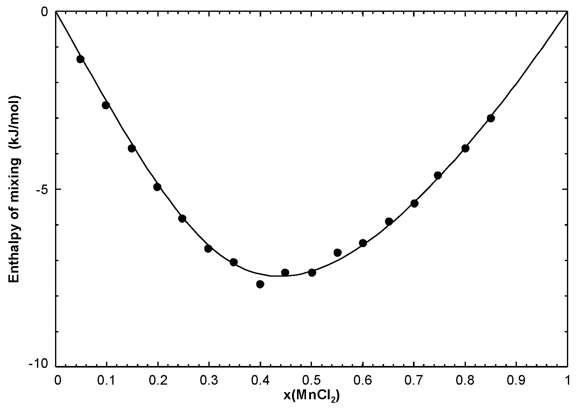
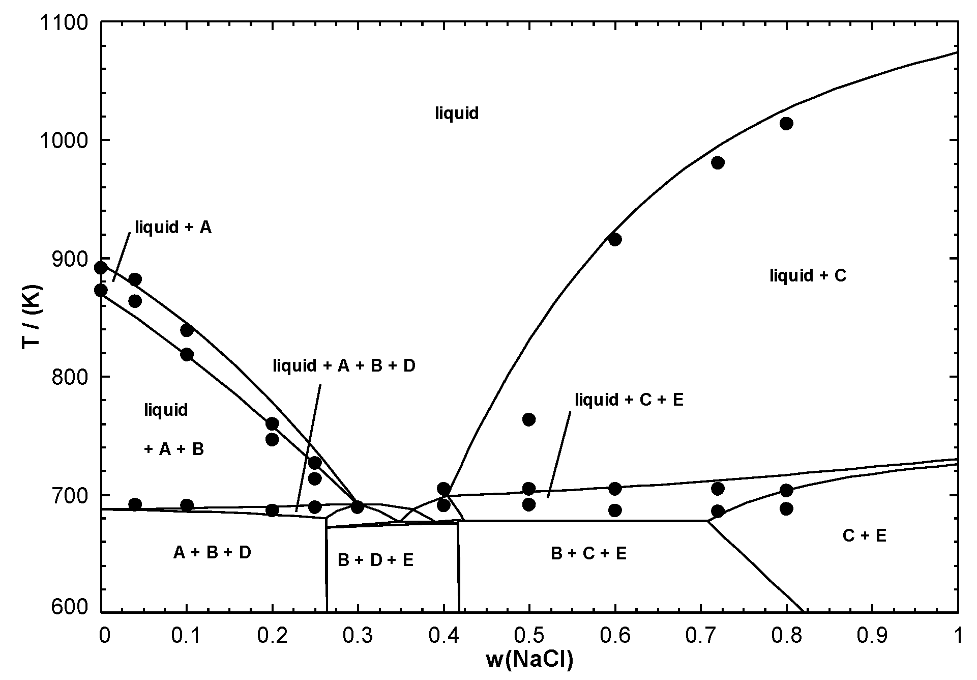
For instance, let us consider the NaCl-MnCl${}_2$ binary system, which was modelled previously [19]. The liquid phase was modelled using the Modified Quasichemical Model for short-range ordering [16], and an expression of its Gibbs free energy as a function of temperature and composition was obtained. The calculated phase diagram, enthalpy of mixing of the liquid at 1083.15 K, and activity of NaCl (relative to liquid standard state) in the liquid at 885.15 K and 1085.15 K are shown along with the available measurements in Figure 3, Figure 4, and Figure 5, respectively. As can be seen in Figure 3, there are five stoichiometric compounds (Na${}_6$MnCl${}_8$, Na${}_2$MnCl${}_4$, Na${}_9$Mn${}_{11}$Cl${}_{31}$, Na${}_2$Mn${}_3$Cl${}_8$, and NaMn${}_4$Cl${}_9$). The enthalpies of formation from solid NaCl and MnCl${}_2$ of Na${}_6$MnCl${}_8$, Na${}_2$MnCl${}_4$, Na${}_2$Mn${}_3$Cl${}_8$, and metastable Na${}_9$Mn${}_{11}$Cl${}_{31}$ (ilmenite structure) at 298.15 K have been measured by solution calorimetry. In addition, the Gibbs free energy changes for various reactions of formation of the five intermediate compounds have been measured over specific temperature ranges using an emf technique. All these data are reproduced by the model within the experimental error limits [19]. A similar approach needs to be used for all remaining subsystems of the multicomponent system of interest (i.e., NaCl-MgCl${}_2$, NaCl-CaCl${}_2$, MgCl${}_2$-CaCl${}_2$, MgCl${}_2$-MnCl${}_2$ and CaCl${}_2$-MnCl${}_2$ for NaCl-MgCl${}_2$-CaCl${}_2$-MnCl${}_2$). If only phase diagram data are available for a given binary subsystem, some assumptions may have to be made. For instance, for MgCl${}_2$-MnCl${}_2$, a solid solution was reported over the entire composition range [20]. Thus, in principle, there is an infinite number of sets of excess Gibbs free energy expressions for the solid solution and the liquid phase permitting one to reproduce the experimental phase diagram. However, owing to the very similar cationic radii of Mg${}^{2+}$ and Mn${}^{2+}$ [21], the MgCl${}_2$-MnCl${}_2$ liquid can be assumed to be close to ideality, thus permitting one to model the solid solution unambiguously. Calorimetric measurements at 1083.15 K exhibiting a maximum enthalpy of mixing of about 350 J/mol confirm the validity of this assumption [20]. For a given binary subsystem, if there are only liquidus data and if negligible solid solubility is observed, then only the chemical potentials of the two components in the liquid phase along the liquidus are defined. In that case, in the absence of enthalpy of mixing data, only enthalpic parameters without any excess non-ideal entropic parameters ought to be introduced in the optimized excess Gibbs free energy of the liquid phase. Finally, if phase diagram data are lacking, estimations might be made from a chemically similar binary system for which such data are available. Although the corresponding results might not be quantitatively accurate, a reasonable trend should be observed.

The third and final step in developing a database for the multicomponent liquid solution is to choose a suitable interpolation method for every ternary subsystem of the multicomponent system of interest, whereby the thermodynamic properties of any ternary subsystem can be estimated from the optimized model parameters of the corresponding binary subsystems. If experimental ternary data are available, then empirical ternary interaction parameters describing the mutual interaction between all three components may be included in the liquid model. All model parameters are stored in a thermodynamic database, and the models can then be used along with a Gibbs free energy minimization software to make predictions in the multicomponent system. For molten salts, the Kohler-like (symmetric) and Kohler–Toop-like (asymmetric) interpolation methods are commonly used [29]. For instance, the NaCl-MgCl${}_2$-CaCl${}_2$-MnCl${}_2$ subsystem comprises the monovalent alkali cation Na${}^{+}$ and the divalent cations Mg${}^{2+}$, Ca${}^{2+}$ and Mn${}^{2+}$. Therefore, the MgCl${}_2$-CaCl${}_2$-MnCl${}_2$ subsystem was designated as symmetric, whereas the three remaining ternary subsystems were asymmetric with NaCl as the asymmetric component [19]. For salt systems, when ternary model parameters are required, both their number and amplitude are often not large. For the NaCl-MgCl${}_2$-CaCl${}_2$-MnCl${}_2$ subsystem, to our knowledge, no ternary data are available in the literature. However, quaternary data were reported [19]. As an example, the calculated section at a constant mass ratio MgCl${}_2$/CaCl${}_2$/MnCl${}_2$ = 1/1/1 is compared with the available measurements in Figure 6. The various solid solutions were modelled with the Compound Energy Formalism [15]. The calculations in Figure 6 were made using only the optimized model parameters for the six binary subsystems; they show that the Modified Quasichemical Model is well suited to perform reliable calculations in multicomponent salt systems. The thermodynamic models for the NaCl-MgCl${}_2$-CaCl${}_2$-MnCl${}_2$ system and for several other chloride, fluoride, and chloro-fluoride systems are available in the FTsalt database of FactSage [4].

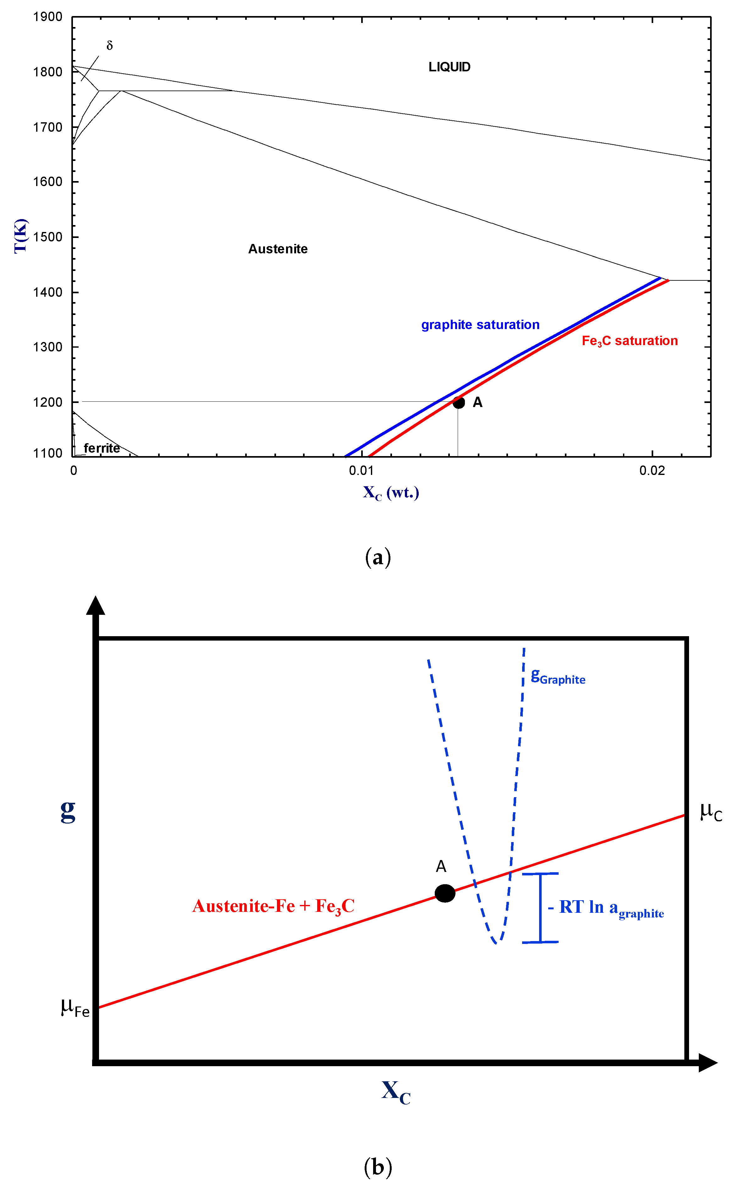
2.3. Stable State vs. Metastable State

A point of fundamental importance when simulating thermodynamic aspects of a real-life pyrometallurgical process is to distinguish between stable and metastable phases. It is common that a thermodynamically stable phase cannot form because of kinetic constraints. The manufacturing of alloys usually involves the generation of a liquid phase followed by its rapid solidification. At this point, the material is thermodynamically unstable and requires energy to reach a desired pseudo-stable state. Heat treatments are subsequently performed to enhance solid diffusion and to promote phase transitions. As an example, carbon saturation in iron is typically defined in metallurgy by establishing a metastable equilibrium with cementite (Fe${}_3$C). Graphite, which can lower the Gibbs free energy of the system, is not easily formed. Figure 7a shows the Fe-C phase diagram calculated using graphite (blue line) and cementite (red line), respectively, as the C-saturating phases. At a temperature of 1200 K, the carbon solubility in Fe-FCC is lower when graphite is considered as it is slightly more thermodynamically stable than cementite.

It is possible to account for the metastability of a given phase by considering it as dormant in an equilibrium calculation. In this calculation mode, the dormant phase is not part of the phase assemblage, but its activity (also called affinity) is evaluated [3]. Figure 7b illustrates graphically how to calculate the activity of a dormant phase—in this case, graphite. The red line in this figure defines the Gibbs free energy hyperplane of the metastable equilibrium state (with ${\mu }_i$ the chemical potential of species i), while the blue line defines the Gibbs free energy of the dormant phase (in this case graphite). The calculation of a phase activity ultimately allows the evaluation of the thermodynamic driving force ($\Delta g_{DF}$) for the formation of this dormant phase, which is expressed as follows:

$$\Delta g_{DF}=-RTln\left(a_{i,Dormant}\right)$$

(5)

Equation (5) shows that the closer the activity of the dormant phase is to unity, the smaller is the thermodynamic driving force for its formation. In our example (i.e., Figure 7b), dormant graphite has an activity of 1.06 at 1200 K at cementite saturation, which represents a small thermodynamic driving force for its formation. A phase with an activity that is lower than one is not stable.

2.4. Isobaric-Isothermal NPT Ensemble Phase Equilibria

At the atomic scale, the available internal energy U of a given chemical system is quantified by a potential contribution ($U_{pot.}$) and a kinetic contribution ($U_{kin.}$). The potential internal energy arises from the chemical interactions (i.e., electromagnetic forces) between the species that constitute the system while the kinetic internal energy is a direct consequence of the atomic vibration induced by temperature. The first law of thermodynamics defines how this state property changes as a function of the imposed conditions. For a reversible process performed on a closed system, this can be expressed as follows:

$$dU=TdS-PdV+\sum _i{\mu }_{i}d{n}_i$$

(6)

The entropy S and volume V are rarely controlled parameters in real-life applications. Pyro-metallurgical reactors are most of the time controlled by constraining their temperature T, their pressure P, and their mass balances that are expressed using a vector n. In this case, the Gibbs free energy G is the adequate thermodynamic function to be analyzed:

$$dG=-SdT+VdP+\sum _i{\mu }_{i}d{n}_i$$

(7)

The basis of computational thermochemistry is therefore to define the Gibbs free energy of the system $G_{system}\left(T,P,\mathbf{n}\right)$.

2.5. Thermodynamic Constraints Used in Process Simulations

One misconception about computational thermochemistry is that it cannot represent a dynamic system that has not reached its equilibrium state. At any time t, classical thermodynamics will correctly define the state of the system if adequate constraints are used to perform the equilibrium calculations. These constraints can be deformations ${ϵ}_i$, stresses ${\sigma }_i$, chemical potentials ${\mu }_i$, molar ratios $\frac{n_i}{n_j}$, etc. The challenge is then to identify which constraints need to be applied to evaluate the equilibrium state at time t.

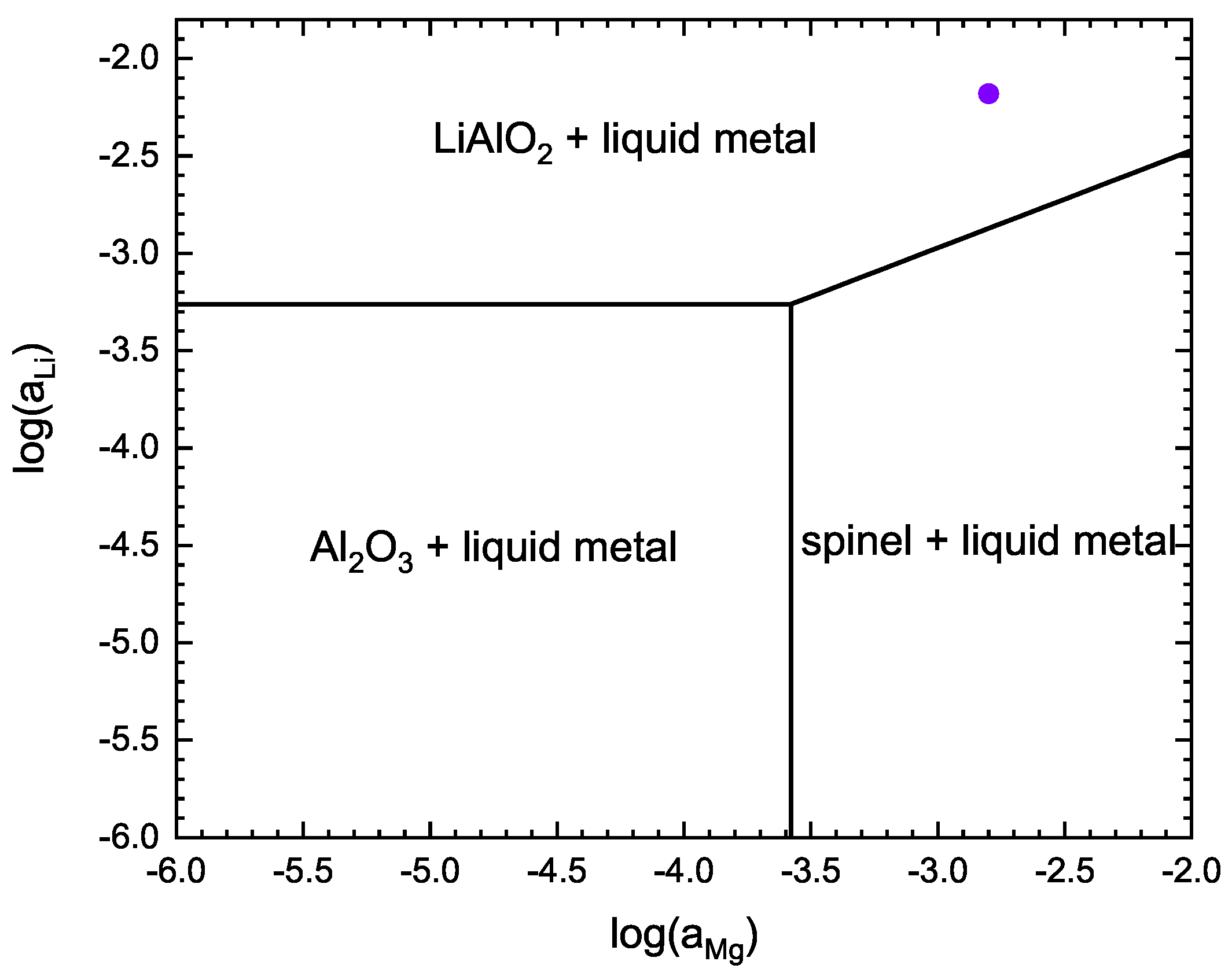
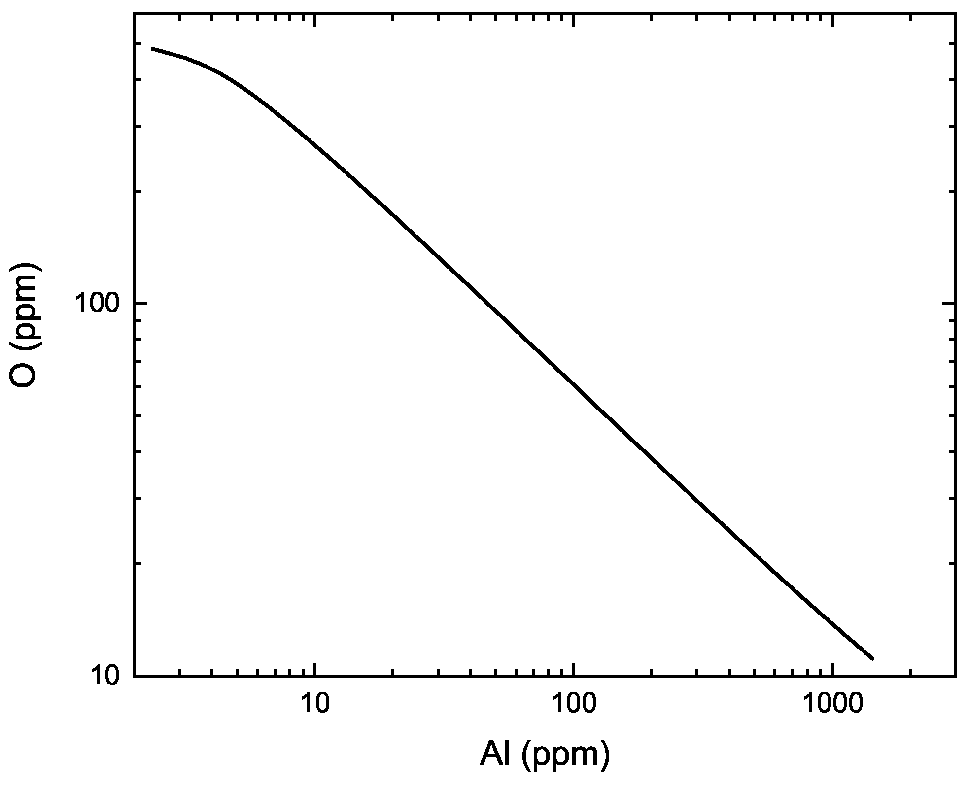
In pyro-metallurgical applications, chemical potentials ${\mu }_i$ (not mass balances) are often required to constrain the phase assemblage evolution of a system. The corrosion of refractories by a molten alloy is a perfect example. In this case, there is always enough mass of the reactive/corrosive element(s) to promote the surface reaction. The growth of the corrosion product layer will be limited by diffusion (Figure 8).

For completely solid systems that are initially not at equilibrium, it is also possible to identify elements that diffuse substantially faster than others. Diffusion of carbon and hydrogen in austenitic stainless steels via interstitial site displacements is one example. In this case, we assume that the molar ratios of the non-diffusing elements (i.e., Fe, Cr, Ni) are constant. This type of constrained calculations is called para-equilibrium and is of prime importance in the thermodynamic study of metallic materials. It is to be noted that it is also possible to constrain the chemistry of a given phase to match for example experimental evidence.

Finally, with the advent of new thermodynamic models of solid solutions that explicitly account for the effect of atomic inter-distances in the description of the enthalpy, we can now impose volumetric constraints to solidified alloys to predict their initial state. The stored internal potential energy released upon heat treatments and the resulting phase transitions can be evaluated with this approach.

3. Computational Thermochemistry in Materials Science

3.1. Differential Scanning Calorimetry and Thermal Analyses

We recently discussed the importance of experimental data obtained by Differential Scanning Calorimetry (DSC) and Thermogravimetric analyses (TGA) [31] to determine the Gibbs energy of stoichiometric phases (i.e., Equation (1)).

TGA is used to study the thermal decomposition behavior of compounds that involves the formation of a gas phase. Upon thermal decomposition, the gas evolving as a result of this first order phase transition will leave the system via the inert carrier gas flowing in the analyzer. This results in a mass loss of the sample which is recorded by a high precision balance. Figure 9 shows the mass evolution of a CuSO${}_4$(H${}_2$O)${}_5$ sample performed using a LabSys-Evo DSC-TGA at a heating rate of $5\frac{K}{min}$ using a flow of argon. The following chemical reaction sequence defines the thermal decomposition mechanism of this compound:

$$CuS{O}_4{\left(H_{2}O\right)}_5\left(s\right)\to CuS{O}_4\left(H_{2}O\right)\left(s\right)+4H_{2}O\left(g\right)$$

(8)

$$CuS{O}_4\left(H_{2}O\right)\left(s\right)\to CuS{O}_4\left(s\right)+H_{2}O\left(g\right)$$

(9)

$$2CuS{O}_4\left(s\right)\to \left(CuO\right)CuS{O}_4\left(s\right)+S{O}_2\left(g\right)+0.5O_2\left(g\right)$$

(10)

$$\left(CuO\right)CuS{O}_4\left(s\right)\to 2CuO\left(s\right)+S{O}_2\left(g\right)+0.5O_2\left(g\right)$$

(11)

We also present in this figure thermodynamic simulations performed using the FactPS (pure substances) database of FactSage in the open calculation mode. This type of calculation proceeds as follows: an imposed amount of gas is first introduced into the system. This gas phase is then allowed to equilibrate with the solid to be thermally decomposed at some imposed temperature and pressure. Finally, the equilibrated gas phase is removed from the system and the process is repeated until the final conditions are reached.

By modulating the proportion of gas to solid in equilibrium at each time t, one can reproduce the experimental TGA weight loss signal as seen in Figure 9. This thermodynamic simulation therefore provides information about the thermal decomposition kinetics via the identification of the gas to solid ratio needed to reproduce the experimental data.

A DSC measures a heat flow signal associated with a sample’s response to a thermal program that includes a specific heating rate $\lambda$. The measured heat flow $\dot{Q}$ (generally expressed in mW) is obtained after a calibration of the equipment which allows a conversion of the raw signal measured in $\mathsf{\mu }$V. Figure 10 shows a DSC experiment performed on a 2024 commercial aluminum alloy (4.3Cu-1.25Mg-0.4Mn). In this figure, the heat flow signal has been converted into a specific isobaric heat capacity of the system via the following equation:

$$\frac{\dot{Q}}{m}·\frac{1}{\lambda }={\left(\frac{\partial h}{\partial t}·\frac{\partial t}{\partial T}\right)}_P=c_P$$

(12)

In theory, it is possible to predict this DSC signal from standard NPT thermodynamic calculations as it is directly related to the isobaric heat capacity of the system. Figure 10 plots the evolution of $c_P$ as a function of temperature as predicted from the FactSage FTlite database that is specifically developed to explore the thermodynamic behavior of aluminum alloys. We predict with this database a liquidus temperature of the 2024 alloy at 915.05 K, which is 7 K below the measured value obtained with a DSC-rod. It is to be noted that other transitions in the solid phase occur below the liquidus temperature (see

Table 3. Evolution of phase assemblage of a 2024 commercial alloy with temperature (cooling) as predicted by the FTlite database of FactSage.

Temperature Range (K)	Phase Assemblage
$T>915.05$	$liquid$
915.05–908.05	$FCC+liquid$
908.05–784.25	$FCC+A{l}_{7}C{u}_{2}Mn\left(E{9}_a\right)+liquid$
784.25–783.35	$FCC+A{l}_{2}Cu\left(C16\right)+A{l}_{7}C{u}_{2}Mn\left(E{9}_a\right)+liquid$
783.35–687.15	$FCC+A{l}_{2}Cu\left(C16\right)+A{l}_{7}C{u}_{2}Mn\left(E{9}_a\right)$
687.15–561.15	$FCC+A{l}_{2}Cu\left(C16\right)+A{l}_{7}C{u}_{2}Mn\left(E{9}_a\right)+A{l}_{2}CuMg$
561.15–298.15	$FCC+{(Al,Cu)}_{2}Mg\left(C14\right)+A{l}_{2}Cu\left(C16\right)+A{l}_{7}C{u}_{2}Mn\left(E{9}_a\right)$

). The corresponding signals are not detected because the enthalpy changes associated with the transitions are relatively small, as predicted by the calculated $c_p$ evolution.

3.2. Multi-Objective Materials Selection

In many industrial problems, one of the key limiting factors of the process design is the optimal material selection for critical applications such as heat exchange tubes, vessel linings, valves, and heat transfer fluids. In most cases, the objective is to predict the material compositions minimizing, maximizing, or targeting a set of thermodynamic, mechanical, and physical properties.

Finding the optimal temperature and pressure process conditions is also highly desirable. In principle, one could use FactSage to identify optimal compositions of a multicomponent solution by simply calculating the properties of interest over a compositional grid. Obviously, such an approach is extremely time-consuming and would be applicable for low-order systems only since the number of calculations necessary to reach the optimal function increases exponentially with the number of components in the system. Calculating optimal alloy compositions and process conditions within a reasonable calculation time is possible with the FactOptimal module [32,33,34,35] for systems with up to 15 to 20 components, depending on the number of phases involved.

The FactOptimal module is integrated into the equilibrium calculation module of FactSage. FactOptimal is based on the Mesh Adaptive Direct Search algorithm (MADS) [36] designed for solving optimization problems when the objective functions and the constraints defining the problem are outputs of a computer simulation—in this case, FactSage. The use of a direct search method algorithm, such as MADS, is particularly relevant in optimization problem when (i) evaluating the considered functions is potentially costly and may even fail in a certain domain, (ii) both objective functions and constraints have no structure which would permit the calculation of derivatives and (iii) the functions and/or constraints are defined in certain regions only with a non-defined pattern. Typical thermodynamic properties are: phase volume fractions, liquidus and solidus temperature, activity, enthalpies, heat capacities, etc. Note that, contrary to other optimization algorithms such as genetic algorithms, the MADS algorithm is not a heuristic approach since a rigorous convergence analysis based on non-smooth calculus is considered in the optimization procedure. FactOptimal has proven itself in several real-world engineering applications [32,33,34,35,37,38].

To illustrate the strength of the FactOptimal software module, we present two examples with potential applications here. The first example is the identification of all local minima on the liquidus surface in multicomponent systems. Local minima on liquidus surface can be eutectics, simple minima (azeotrope-like), or saddle points. The knowledge of such special compositions has many industrial applications: solders, heat storage materials, transfer media, or casting fluxes. The FactOptimal methodology allowing the determination of local minima on the liquidus surface of multicomponent systems has been presented in our prior works [34,38] and will not be repeated here. All local minima in the LiF-NaF-KF-MgF${}_2$-CaF${}_2$-SrF${}_2$-BaF${}_2$ system have been calculated. A total of 183 local minima on the liquidus surface were identified, including all subsystems (unaries, binaries, ternaries, etc.) of the seven-component system. In Figure 11, the minimum liquidus temperatures of all identified compositions are represented as a function of their corresponding enthalpy of melting. Each point represents a different composition with different properties. The absolute minimum liquidus temperature for this system is 720 K (447 ${}^{\circ }$C) while the maximum enthalpy of melting is 60 kJ/mol. Although the general trend is a linear increase of the enthalpy of melting with liquidus temperature, a large dispersion is observed.

In the second example, we illustrate the FactOptimal software module to the improvement of mechanical properties of FeCoCrNiMn high entropy alloys (HEA) by carbon doping. In principle, a high entropy alloy is constituted of five or more elements in near equiatomic proportions. Nevertheless, nowadays, HEA research aims more and more at finding potential candidates outside of the equiatomic composition. In general, HEAs have a single FCC or BCC phase, even though some dual FCC+BCC phases HEAs could be of interest. FeCoCrNiMn is one of the most promising candidates for future industrial applications of high entropy alloys [39]. Equiatomic FeCoCrNiMn has a FCC single phase in the temperature range: 923 K ≤ T ≤ 1552 K [37]. The lowest temperature of this range is called the single-(FCC)phase start temperature (SPST). This value is relatively high for FeCoCrNiMn (923 K). Having the lowest SPST possible is highly desirable as it minimizes the thermal activation energy available for undesirable solid–solid phase transitions to occur below this temperature. Peng et al. [40] have demonstrated that carbon doping improves the mechanical properties of FeCoCrNiMn, strengthening it by the precipitation of M${}_{23}$C${}_6$ carbides and inhibiting the recrystallized grain growth of the FCC matrix. Peng et al. [40] only studied the specific composition FeCoCrNiMn-1.3C. We intend to optimize the mechanical properties of FeCoCrNiMn by carbon doping. However, in order to conserve the other good physical properties, the FCC phase should be present at very close to 100 %. The optimization problem is defined as follows:

• Objective functions to optimize:

  -

  Maximizing the amount of M${}_{23}$C${}_6$

  -

  Minimizing the SPST

• Constraints:

  -

  $0.15\le X_{Fe};X_{Co};X_{Cr};X_{Ni};X_{Mn}\le 0.25$

  -

  $X_C\le 0.025$

  -

  $mol\%FCC\ge 99.5\%$

  -

  No precipitate in the FCC matrix other than M${}_{23}$C${}_6$

Note that the constraints are somewhat arbitrary.

The optimal compositions, SPST and M${}_{23}$C${}_6$ mole fraction satisfying the optimization problem defined above are calculated by FactOptimal as:

$$\mathrm{Optimal}=\left\{\begin{array}{c}\mathrm{composition}:\{X_{Fe}=0.185;X_{Co}=0.191;X_{Cr}=0.172;X_{Ni}=0.225;X_{Mn}=0.226;X_C=0.001\}\hfill \\ SPST=825K\hfill \\ X_{M_{23}{C}_6}=1.85\times {10}^{-4}\hfill \end{array}\right.$$

(13)

3.3. Refractory Crucible Selection for High Temperature Applications

The operation of high temperature pyrometallurgical processes nearly always involves the formation of chemically aggressive liquid phases (i.e., slag, matte, speiss, liquid metal, molten salts, etc). In specific cases such as ilmenite reduction in an electrical arc furnace, the liquid phase is so aggressive that the only option to contain it is by freezing it on the surface of the vessel using, for example, water-cooled copper plates [41]. Hence, the optimal selection of lining materials of high-temperature pyrometallurgical reactors is a critical task to limit shutdowns and prevent catastrophic accidents. At a smaller scale, an appropriate selection of crucibles used in high temperature experiments (such as DSC) is also of prime importance to avoid composition shifts of the samples as well as expensive equipment failure.

The Ellingham diagram is a simple graphical tool that provides the standard Gibbs energy of formation of oxides and sulfides. These diagrams can be used to determine the compatibility between a liquid metal and a solid oxide refractory. This type of diagram generally assumes the formation of pure compounds and cannot directly predict the complex behavior of a system in which solid and liquid solutions may form. The correction of these standard Gibbs energy of formation expressions to account for the activity of the reactants and products in solutions can be a laborious task [42]. The coupling of the FToxid and FTlite databases provides a powerful tool to identify the best refractory material to be used for a given application.

In our first example, we evaluate the compatibility between liquid nickel and alumina. This is an important system as nickel is typically used as a standard material to calibrate (via its melting) high temperature DSC equipment. According to the standard Ellingham diagram of oxides, alumina is an adequate material to contain nickel. In the absence of oxygen excess, FactSage predicts that an equilibrium between liquid nickel and alumina is established at 1873.15 K and 1 atm. In these conditions, a spinel solid solution thermodynamically described in the FToxid database has an activity of 1 and should be stable as well. Any excess of oxygen in the system promotes the formation of this spinel solid solution (with NiAl${}_2$O${}_4$ as the main component of this phase which melts around 2383.15 K [43]) via the following reaction:

$$Ni\left(l\right)+A{l}_2{O}_3\left(s\right)+0.5O_2\left(g\right)\to NiA{l}_2{O}_4\left(s\right)$$

(14)

This result has been validated during some of our DSC experiments as seen in Figure 12. Ultra-pure metallic Ni partially reacted with the alumina crucible to form the blue-green spinel phase. It is to be noted that the same behavior occurred when using ultra pure Co as a reference material to calibrate the DSC.

In the second example, we use FactSage to select the optimal refractory crucible (by comparing the behavior of SiO${}_2$, TiB${}_2$ and Al${}_2$O${}_3$) to synthesize the new AA2027 Al-Cu-Li alloy recently proposed by Miao et al. [44]. The nominal composition of this alloy is presented in

Table 4. Nominal composition of a new AA2027 alloy proposed by Miao et al. [44].

Element	Cu	Li	Mg	Mn	Zn	Zr
wt.%	3.11	0.65	0.18	0.26	0.32	0.12
Vapor pressure (bar) at 1068.15 K	5.7 × 10${}^{-14}$	2.2 × 10${}^{-5}$	6.6 × 10${}^{-5}$	4.0 × 10${}^{-12}$	7.7 × 10${}^{-4}$	-
$a_i(liq.)$(ref. pure liq.) at 1068.15 K	2.1 × 10${}^{-4}$	6.6 × 10${}^{-3}$	1.6 × 10${}^{-3}$	1.3 × 10${}^{-5}$	2.6 × 10${}^{-3}$	8.8 × 10${}^{-8}$

. The FTlite database predicts a liquidus temperature for this alloy at 968.15 K with Al${}_3$Zr-D0${}_{23}$ precipitating as the primary phase. The spherical shape of the Al${}_3$Zr nanoparticles observed by Miao et al. using a transmission electron microscope strengthens the validity of our calculations. This table also shows the vapor pressure of each alloying element at 1068.15 K. During the processing of the alloy in the liquid state, Zn and Li may be partially lost to the atmosphere as they present a significant vapor pressure under these conditions. According to Table 4, the vapor pressure of Mg is even higher than that of Li.

We explore in Figure 13 the behavior of two crucible candidate materials, i.e., SiO${}_2$ and TiB${}_2$. These materials are exposed to a varying quantity of the AA2027 liquid alloy at 1068.15K. The thermodynamic calculations performed in this figure assume that the interactions between the liquid metal and the refractory materials are not diffusion-limited (i.e., the imposed mass balances are respected). As expected from the Ellingham diagram, SiO${}_2$ is not a good candidate to contain liquid aluminum since silicon is more noble than Al. Consequently, any small quantity of SiO${}_2$ will react with the liquid alloy to form Al${}_2$O${}_3$ while transferring silicon to the liquid metal. In this specific example, the presence of lithium, a reactive and fast-diffusing metal, leads to the formation of another corrosion product, LiAlO${}_2$. Lithium depletion in the liquid alloy occurs as soon as it is in contact with SiO${}_2$. The behavior of TiB${}_2$ is completely different. According to Figure 13, this material is almost completely inert toward this liquid aluminum alloy. In fact, the only reaction that occurs is zirconium transfer from the liquid alloy to the TiB${}_2$ material combined with a transfer of titanium to the melt (Figure 13D).

In the eventuality that the chemical interactions are limited by diffusion (see the schematic in Figure 8), it is difficult to define the appropriate mass balances to be imposed on the system. In this case, it is better to produce a phase mapping such as the one presented in Figure 14. In this figure, we assume that only Li and Mg can diffuse in the refractory material. In this scenario, the LiAlO${}_2$ phase forms at 1068.15 K when the chemical potentials of Li and Mg of the AA2027 liquid alloy are imposed on the system. It is to be noted that the formation of the less dense LiAlO${}_2$ induces a substantial volumetric change of the alumina matrix which favors its cracking.

3.4. Anodic/Cathodic Polarization Simulations

High temperature electrochemical processes are important technologies for the circular economy of the future. They theoretically allow separation and recovery of multiple elements present in an electrolyte which can be solid or liquid. The identification of the anodic and cathodic reactions occurring in a system as a function of the imposed voltage is at the heart of any electrochemical process. Polarization tests are commonly performed to identify these reactions at the anode and the cathode. Polarization is a broad term used to describe the sum of overvoltage contributions. Three main mechanisms are reported by Schwartz [45]: (i) activation polarization, (ii) resistance polarization, and (iii) concentration polarization. The first contribution is associated with the kinetic barriers of the charge transfer reaction. Resistance polarization describes many phenomena; for instance, the passivation of the electrode with an oxide layer or the presence of a gas film (such as H${}_2$(g)) at its surface in aqueous electrolysis. The last contribution is attributed to the change in ion concentrations at the electrodes; this kind of polarization occurs as the boundary layer is depleted of ions as the reaction occurs faster than the mass transfer. To reduce such phenomena, the cell can be run at higher temperature or the electrolyte can be stirred [45].

Polarization curves in electrochemistry are usually represented by plotting the potential (Volts) against the current density (A$·$cm${}^{-2}$). They are obtained using a 3-electrode setup (see Figure 15) by sweeping the applied voltage by a potentio-static power source between a reference electrode and a working electrode and by measuring the current flowing between the working electrode and the counter electrode. In this method, the determination of the electrode surface (cm${}^2$) is necessary to calculate the current density. According to Flitt and Schweinsberg [46], it is often difficult to interpret the anodic and cathodic reaction mechanisms in those experiments. We will show here how classical thermodynamics can be used to identify the chemical reactions occurring at a specific electrode and to visualize the impact of the concentration polarization.

In our example, we firstly explore the anodic polarization of a (Al${}_{0.969}$Mg${}_{0.01}$Mn${}_{0.015}$Si${}_{0.006}$)${}_{wt.}$ liquid aluminum alloy anode in contact with an equimolar NaCl-MgCl${}_2$ electrolyte using the FactPS (gas phase), FTsalt (molten electrolyte), and FTlite (liquid metal and intermetallic) databases. This liquid aluminum alloy represents the nominal composition of a used beverage can (UBC). The recycling strategy of UBCs proposed in the literature often involves Mg removal using electrolysis in molten chloride salt performed at around 973.15 K [47]. The Ag/AgCl reference electrode is used here to evaluate the anodic polarization. The mass transfer of chlorine ions is imposed by the $\alpha$ amount of AgCl(l) added to the system.

Table 5. Anodic and cathodic polarization simulation parameters performed using the FactPS, FTlite, and FTsalt databases at 973.15 K and 1 atm.

	Reactants	Amount (g)	Specific Gibbs Free Energy (J/g)
Anode
	$\left(A{l}_{0.969}M{g}_{0.01}M{n}_{0.015}S{i}_{0.006}\right)(liq.)$	100	−1551.4
	+
	$(0.5NaCl-0.5MgC{l}_2)(liq.)$	100	−8507.2
	+
	$AgCl(liq.)$	$\alpha$	−1760.3
Cathode
	$(0.49NaCl-0.51MgC{l}_2)(liq.)$	100	−8501.5
	+
	$Ag\left(s\right)$	$\alpha$	−499.9

presents the specific Gibbs free energy of the reactants to be used to calculate the anodic polarization voltage, which is calculated as follows:

$$E=-\frac{\Delta G}{n·F}$$

(15)

The phase selection in these calculations is particularly important in this case since we want to force the reaction of the reference electrode:

$$AgCl(liq.)+1e\to Ag\left(s\right)+C{l}^{-}$$

(16)

Since the Ag/AgCl reference electrode is not a part of the reactive system, it is necessary to remove Ag-based species from the calculations in all the selected solutions, notably in the liquid alloy, in the molten salt and in the gas phase. Similarly, all the Ag compounds need to be deactivated so that only pure Ag can precipitate in the reference electrode. It is then possible to calculate a concentration polarization curve for the anodic component of the cell. Figure 16A shows that the Mg is transferred from the liquid anode to the electrolyte (in the form of MgCl${}_2$) as the charge transfer is increased, which is reasonable since it is the most reactive metal in the UBC alloy. It can be seen in this figure that the anode potential drastically changes when the charge transfer is high enough to oxidize all the Mg (Figure 16B), which leads to a transfer of aluminum to the electrolyte (in the form of AlCl${}_3$).

A similar procedure is applied for simulating the cathodic polarization of the cell. In this case, only AgCl(liq) is selected as a stable Ag-based phase product to force the inverse of reaction (16). The electrolyte composition at the cathode used to perform these calculations is 0.49NaCl-0.51MgCl${}_2$ since some MgCl${}_2$ is transferred at the cathode. Figure 16C shows the linear decrease of the cathodic polarization to produce pure liquid magnesium as a function of the charge transfer, which is induced by the shift in composition of the electrolyte as liquid Mg is produced. Finally, Figure 16D shows the amount of liquid Mg produced at the cathode as a function of the charge transfer.

4. Computational Thermochemistry to Simulate Smelting and Refining Processes

4.1. Al-Operating Conditions of the Hall–Heroult Process

This section presents different thermodynamic simulations performed with the FactSage FThall database, which is specifically developed to model the Hall–Heroult (HH) cell. This process produces liquid aluminum from the electrochemical smelting of alumina dissolved in a cryolitic bath using graphite anodes. Some critical thermo-physical properties of a typical cryolitic bath used in the industry (i.e., 10 wt.% AlF${}_3$, 5 wt.% CaF${}_2$ and 3 wt.% Al${}_2$O${}_3$) calculated using the FThall database are presented in

Table 6. Theoretical operating conditions of the Hall–Heroult cell based on thermodynamic calculations performed using the FThall database.

Property	Value
Cryolite bath (wt.)—$82N{a}_{3}Al{F}_6+10Al{F}_3+5Ca{F}_2$
$T_{liquidus}$ (no $A{l}_2{O}_3$ dissolved)	1254.45 K
density (at $T_{liquidus}$)	2098 kg$·$m${}^{-3}$
$A{l}_2{O}_3$ max. solubility (at $T_{liquidus}$)	9 wt.%
Liquid aluminum
$T_{Melting}$	933.15 K
density (at $T_{Melting}$)	2380 kg$·$m${}^{-3}$
Na solubility (equilibrium with cryolite bath at $T_{liquidus}$)	64 ppm (wt.)
Cell operation—(3 wt.% Al${}_2$O${}_3$ at 1253.15 K)
Cryolite $T_{liquidus}$	1235.25 K
Al${}_2$O${}_3$ activity (ref. solid corundum) in cryolite	0.09
cryolite density	2068 kg$·$m${}^{-3}$
molten Al density	2290 kg$·$m${}^{-3}$

. According to this table, the minimum operating temperature for this HH cell is 1235.25 K if alumina is continuously fed to the cell to maintain its concentration. An alumina depletion will increase the liquidus temperature of the system up to 1254.45 K. This situation should be avoided as it leads to an anode effect. Under normal operating conditions of the cell, the cryolite density is lower than that of the liquid metal. This ensures a physical separation between the two liquid phases.

Simulation of the Overall Electrochemical Process

The overall reaction that defines the HH process is the following:

$$2A{l}_2{O}_3\left(s\right)+3C\left(s\right)\stackrel{1253.15\mathrm{K}}{\to }4Al(liq.)+3C{O}_2\left(g\right);\Delta G^0\left(1253.15\mathrm{K}\right)=1366\mathrm{kJ}$$

(17)

Under normal operating conditions, the required electrical work (i.e., $\Delta G$) of the HH process imposes the theoretical voltage to apply to the HH cell, which can be calculated via the Nernst equation:

$$-nFE=\Delta G^0+RTln\left[\frac{{\left(P_{C{O}_2}\right)}^3}{{\left(a_{A{l}_2{O}_3}\right)}^2}\right]\to E=-1.22\mathrm{V}$$

(18)

In Equation (18), we used a partial pressure of CO${}_2$ ($P_{C{O}_2}$) of 0.9 atm as reported by Aarhaug and Ratvik [48] as well as the alumina activity presented in Table 6. To this theoretical voltage of −1.22 V, the anodic and cathodic over-potentials as well as the voltage induced by the Joule effect need to be added.

In order to get a more precise understanding of what is occurring at both the anode and the cathode, a simulation of the electro-migration processes occurring in the HH cell is explored. In Figure 17, we assume that the majority of the charge transfer is made by sodium cations and fluorine anions. In the literature, it is reported that about 90% of the charge is transferred by Na${}^{+}$ ions and about 10% by F${}^{-}$ ions [49,50,51,52,53]. The thermodynamic calculations are performed on a basis of 100 g of electrolyte. At the anode, we remove 0.9$\alpha$ moles of Na${}^{+}$ and add 0.1$\alpha$ mole of F${}^{-}$, respectively, to mimic the electro-migration process (basis of 1.0$\alpha$ mole of charge). Assuming that each mole of carbon transfers four moles of electrons upon its oxidation to form CO${}_2$(g), we also include 0.25$\alpha$ moles of carbon (which will be consumed) at the anode. At the cathode, the sign of the Na${}^{+}$ and F${}^{-}$ ions fluxes is inverted so that the overall mass balance of the electrolyte is not altered by the electro-migration process.

The evolution of the chemical composition of the exhaust gas at the anode as a function of $\alpha$ is presented in Figure 18A. Under normal operating conditions, CO${}_2$(g) is the major species in the gas phase. In this example, we did not use any excess carbon, which prevents the formation of CO(g) in our simulations through the Boudouard reaction, i.e., $C{O}_2\left(g\right)+C\left(s\right)\to 2CO\left(g\right)$. According to this figure, an anode effect starts when more than 0.17 mole of charge migrates in the system (for a basis of 100 g of electrolyte). After this point, the amounts of COF${}_2$ and CF${}_4$ in the gas phase sharply increase. At the cathode, liquid aluminum is produced for all explored conditions. The amount of Na dissolved in the Al(liq) increases with the amount of charge migrating in the system as can be seen in Figure 18B. Finally, the change in the anodic reaction at high charge transfer is evident in Figure 18C, which presents the evolution of the theoretical voltage as a function of the charge transfer in the system.

4.2. Ni Laterite Reduction

Nickel is an important metal used in many high-tech materials such as austenitic stainless steels and nickel superalloys to produce turbines and other critical components of power stations and jet engines. We simulate here the primary nickel production from laterite ores using the PTVI process as data can be found in the literature. These simulations are performed with the FTmisc, FToxid, and FactPS databases. When possible, we compare our results with the available experimental data of the real-life process found in the literature. As seen in Figure 19, the PTVI process includes four major metallurgical steps, i.e., (i) drying, (ii) calcination, (iii) smelting, and (iv) converting. This simplified flowchart also shows the reactants and product streams for each unit. In the first simulation step, a wet lateritic ore composition (

Table 7. Stream properties of the PTVI process

Stream ID	Flow Rate (t/h)	Composition (wt.%)	Phase Assemblage
Wet Laterite
I1 (298.15 K, 1 atm)	955	(2.75NiO-27.4FeO-39SiO${}_2$	[olivine+spinel +Mg${}_3$Si${}_2$O${}_5$(OH)${}_4$
		-20.5MgO-0.1CoO-10.25H${}_2$O)	+Mg${}_3$Si${}_4$O${}_{10}$(OH)${}_2$+H${}_2$O(ab.)
			+trace of FCC]
Dryer kiln (393.15 K)
O1	44.9		gas
IS1	910.1		[spinel +Mg${}_3$Si${}_2$O${}_5$(OH)${}_4$
			+Mg${}_3$Si${}_4$O${}_{10}$(OH)${}_2$]
Calcination kiln (973.15 K)
I2	34.13		C (from coal)
I3	1.5		S(from HSFO)
O2	91.7		gas
IS2	854.1		[Orthopyroxene+olivine+Ni${}_3$S${}_2$
			+FCC + C]
I4 (Added to the kiln discharge)	12		molten sulfur
Smelter (1788.15 K)
I5	7.05		graphite
O3	25.3		gas
O4	770.9	0.02Ni-25.5FeO-25.1MgO-47.8SiO${}_2$	slag
		(0.15Ni-23FeO-23MgO-48SiO${}_2$) [54]
IS3	77.0	26.6Ni-63.4Fe-0.8Co-8.7S	matte
		(26Ni-63Fe-0.8Co-10S) [54]
Converter (1723.15 K)
I6	20.3		O${}_2$
I7	45		SiO${}_2$
O5	6.2		gas
O6	114.3	3.8Ni-42.4Fe-39.4SiO${}_2$	slag
		(0.6Ni-53Fe-25SiO${}_2$) [54]
O7	21.7	74.0Ni-1.5Fe-0.4Co-16.4S-7.7O	liquid metal
		(78Ni-1Fe-1Co-20S) [54]

) is used to evaluate the phase assemblage at 298.15 K. The resulting phase assemblage calculated by FactSage is used for the rest of the simulation to define the mass and heat balances. For each unit, the main product stream (identified in red in Figure 19) is sequentially used as a reactant stream for the following unit (i.e., dry kiln product, calcine and furnace matte).

4.2.1. Drying and Calcination

The simulation of the drying unit (T = 393.15 K) shows that most of the absorbed water is removed from the solid stream (IS1). In real-life operating conditions, the dryer is not designed to remove 100% of the moisture; there is typically about 20% of residual moisture [55]. Moreover, handling perfectly dry solids would be almost impossible as excessive dust suspension would form. Under these drying conditions, the Mg${}_3$Si${}_4$O${}_{10}$(OH)${}_2$ and Mg${}_3$Si${}_5$O${}_{10}$(OH)${}_4$ hydrates still remain. The Mg${}_3$Si${}_4$O${}_{10}$(OH)${}_2$ hydrate is predicted to thermally decompose at 579.15 K. The dried product leaves the unit at a temperature of about 343–353 K.

As for the calcination step (T = 973.15K), coal(I2), modelled here as pure carbon, is added to the kiln as a reducing agent for the smelter. It is also to be noted that High Sulfur Fuel Oil (HSFO) was burnt in the past in the kiln to provide the required energy for this operation. The combustion of the HSFO will transfer sulfur to the calcination kiln feed which is represented by the stream (I3) in Figure 19. We estimated that about 1.5 t/h of sulfur is transferred via the combustion of the HSFO. Because of the presence of sulfur in the HSFO, a serious operation problem induced by particle sticking may occur in the kiln if the temperature is too high. According to our thermodynamic calculations, the calcined product starts to melt (i.e., solidus temperature) at 1306.15 K, which imposes a maximum operating temperature for this unit. At a drying temperature of 973.15 K, thermodynamics predicts that all the crystalline water is removed from the charge which is to be compared with a value of about 1% under industrial operating conditions.

4.2.2. Smelting and Converting

The solid products coming out of the calcination kiln (IS2) are introduced into an electric arc furnace. We are aware that part of the solid charge of the kiln (i.e., kiln fines) will be lost to the off-gas. We did not consider this phenomenon in our thermodynamic simulations as it cannot be predicted from computational thermochemistry. The liquid sulfur added at the end of the calcination process in the kiln discharge to ease the formation of a liquid phase inside the electric arc furnace is defined as stream (I4). The reduction inside the furnace is controlled by the amount of carbon in the system (including the electrode consumption I5). The level of reduction in turn defines the nickel recovery as can be seen in Figure 20A. The carbon consumption in this figure includes the amount used to reduce FeO-Fe${}_2$O${}_3$ as well.

Table 7 shows a comparison between the calculated chemistry using FactSage of the resulting matte (IS3) and slag (O4) with typical compositions reported in the literature. Since the control of temperature is a challenge in the electric arc furnace, we performed thermodynamic simulations to evaluate the phase assemblage in the reactor as a function of temperature (Figure 20B). The slag phase starts to form at 1610.15 K. At this temperature, both solid orthopyroxene and olivine remain in the reactor. In fact, the minimal operation temperature of the electric arc furnace for this laterite ore to ensure that only liquid metal (IS3) and slag (O4) are in equilibrium in the reactor is about 1788.15 K.

The last pyrometallurgical operation is the converting which is performed by injecting O${}_2$ (I5) into the reactor and by adding silica as a flux (I6) agent. The final product (O7) composition is in good agreement with the reported data for this process for a converter working at a temperature of 1723.15 K [54]. It is to be noted that the nickel content of the slag dictates its fate: a nickel content above 0.6 wt.% Ni justifies its re-introduction in the calcination kiln while a slag containing less than this value is discarded. Finally, the industrial practice of slag formation in the converter is not a straightforward operation as there are many blowing stages which generate different slag compositions. Therefore, the full equilibrium state is difficult to reach.

4.3. Iron Alloying and Refining

Steel is a technological material used in a panoply of applications. The fine-tuning of steel chemistry is essential to optimize its mechanical performance in a context where its environment in service may be hostile. As an example, the 13Cr-4Ni soft martensitic stainless steel used to build a Francis turbine needs to present good fatigue-resistance properties when exposed to a massive flow of fresh water [56]. Under these operating conditions, pitting corrosion may occur at the surface of the material and promote crack initiation. This steel chemistry is therefore adjusted as follows:

• Chromium is added to form a passive layer at the surface of the alloy to protect it from its environment.
• Nickel, a gamma-stabilizer, promotes the stabilization of austenite.
• Molybdenum is added to strengthen the alloy by solid solution and precipitation of Laves phases [57].

In addition, metal cleanliness is key, as an excessive amount of impurities may lead to the formation of inclusions with deleterious effects (i.e., crack initiation sites, passivation layer discontinuities, etc.). More specifically, carbon and oxygen contents need to be tightly controlled in stainless steels. Carbon content needs to be lowered as much as possible as its presence typically leads to the precipitation of chromium carbides at grain boundaries. This chromium trapping by carbides prevents the formation of a uniform passive layer. Oxygen, which is used to lower the carbon content, also needs to be removed to avoid the excessive formation of inclusions.

Table 8. Summary of the thermodynamic calculation performed for the Fe-13Cr-4Ni-1Mo-0.01C alloy.

Temperature (K)	Phase Assemblage	Comments
1771.15	liquid metal	Fe- BCC is the primary phase
1099.15–1423.15	FCC	Single phase region domain
773.15	BCC + Laves phase + M${}_{23}$C${}_6$

presents important phase equilibria for the Fe-13Cr-4Ni-1Mo-0.01C stainless steel as calculated using the FSstel database. The predicted liquidus temperature of this steel is 1771.15 K. This imposes the minimal operating temperature of the furnace used for the synthesis of the alloy. The BCC iron matrix is the primary phase precipitating from the liquid. The homogenization heat treatment temperature (also called austenitization) can be performed in the range of temperature $\left[1099.15-1423.15\mathrm{K}\right]$. At 773.15 K, thermodynamic calculations predict that the Fe-BCC solid solution (which represents the steel matrix) is in equilibrium with M${}_{23}$C${}_6$ (M = Cr, Fe, Mo) carbides as well as a (Fe,Cr)${}_2$Mo Laves phase induced by the presence of Mo. As reported by Wang et al. [58], the formation of a Laves phase in stainless steel under these conditions is critical, as it may lead to some ageing degradation of the material.

The first step in the thermodynamic simulation of the de-oxidation of the Fe-13Cr-4Ni-1Mo-0.01C steel is to saturate the melt with oxygen (to reach the precipitation of a first solid oxide) to mimic the decarburization process. Figure 21 shows the evolution of the oxygen solubility as a function of temperature as predicted from FactSage using both the FSstel and FToxid databases. Below 1996.15 K, the Cr${}_2$O${}_3$ corundum solid solution saturates the melt, while it is the (Cr,Fe)${}_3$O${}_4$ spinel solid solution at higher temperature. At 1923.15 K (blue circle in the figure), the liquid steel contains 550 ppm (wt.) of oxygen. The second step of the thermodynamic simulation is to react this liquid steel at 1923.15 K with aluminum to lower its oxygen content. In Figure 22, we see how the oxygen solubility in the liquid metal evolves as a function of the aluminum dissolved in the melt. The corundum solid solution that forms as a result of this deoxidation process has a low density and will reach the surface of the melt.

5. Conclusions

In this paper, the relevance of computational thermochemistry is highlighted through specific examples pertinent to materials science and metallurgy. Fundamental concepts of computational thermochemistry are presented beforehand. Concepts such as metastability and paraquilibrium are essential for understanding the results obtained with a computational thermochemistry software such as FactSage.

We have seen that computational thermochemistry can be used to predict the reactions and phase transitions that take place within a system under given NPT conditions. This helps to explore suitable materials for a given application and to avoid wasting time and money in potentially hazardous experiments. It also helps to refine the interpretation of experimental observations, e.g., for the identification of decomposition pathways of a substance in thermogravimetric analysis or of the reactions occurring at the electrodes in electrochemical processes.

A thermochemical calculation software including a suitable optimization algorithm makes it possible to select the composition of an alloy corresponding to a set of criteria given by the minimization of objective functions subject to different constraints. Such an algorithm is essential if Gibbs energy minimization calculations are to be performed for systems comprising a large number of elements and phases. While considering a large number of elements can significantly slow down calculations, it is in some cases an essential measure in order to be able to consider systems that are as realistic as possible in terms of impurity levels, for instance.

Finally, various metallurgical processes were simulated with FactSage. These calculations are only possible if databases containing all the solutions and compounds involved in the processes exist. The accuracy of the results obtained is very dependent on the phases selected in the calculations and the robustness of the models used to describe said phases. The CALPHAD method is used to parameterize thermodynamic models. This method makes it possible to predict the phases in equilibrium in multi-component systems from data on lower order sub-systems. The experimental data used for optimization are critically evaluated and carefully selected to ensure self-consistency.

While the focus was mainly put on alloys and metallurgy, it is to be noted that all the methods shown in this paper can be applied to systems of interest in various other industries (e.g., fertilizers, pulp and paper...), provided accurate databases are available and robust thermodynamic models adapted to the nature of the systems considered are used.

References

1. Eriksson, G.; Thompson, W. A procedure to estimate equilibrium concentrations in multicomponent systems amd related applications. Calphad 1989, 13, 389–400. [Google Scholar] [CrossRef]
2. Eriksson, G. Thermodynamic studies of high-temperature equilibriums. XII. SOLGASMIX, a computer program for calculation of equilibrium compositions in multiphase systems. Chem. Scr. 1975, 8, 100–103. [Google Scholar]
3. Harvey, J.P.; Eriksson, G.; Orban, D.; Chartrand, P. Global minimization of the Gibbs energy of multicomponent systems involving the presence of order/disorder phase transitions. Am. J. Sci. 2013, 313, 199–241. [Google Scholar] [CrossRef]
4. Bale, C.; Belisle, E.; Chartrand, P.; Decterov, S.; Eriksson, G.; Gheribi, A.; Hack, K.; Jung, I.H.; Kang, Y.B.; Melançon, J.; et al. FactSage thermochemical software and databases, 2010–2016. Calphad 2016, 54, 35–53. [Google Scholar] [CrossRef] [Green Version]
5. Dinsdale, A. SGTE data for pure elements. Calphad 1991, 15, 317–425. [Google Scholar] [CrossRef]
6. Leitner, J.; Vonka, P.; Sedmidubsky, D.; Svoboda, P. Application of Neumann-Kopp rule for the estimation of heat capacity of mixed oxides. Thermochim. Acta 2010, 497, 7–13. [Google Scholar] [CrossRef]
7. Burke, K.; Werschnik, J.; Gross, E.K.U. Time-dependent density functional theory: Past, present, and future. J. Chem. Phys. 2005, 123, 062206. [Google Scholar] [CrossRef] [Green Version]
8. Yu, H.S.; Li, S.L.; Truhlar, D.G. Perspective: Kohn-Sham density functional theory descending a staircase. J. Chem. Phys. 2016, 145, 130901. [Google Scholar] [CrossRef]
9. Kim, G.; Meschel, S.V.; Nash, P.; Chen, W. Experimental formation enthalpies for intermetallic phases and other inorganic compounds. Sci. Data 2017, 4, 170162. [Google Scholar] [CrossRef] [Green Version]
10. Blanco, M.; Pendas, A.; Francisco, E.; Recio, J.; Franco, R. Thermodynamical properties of solids from microscopic theory: Applications to MgF2 and Al2O3. J. Mol. Struct. THEOCHEM 1996, 368, 245–255. [Google Scholar] [CrossRef]
11. Seifitokaldani, A.; Gheribi, A.E. Thermodynamically self-consistent method to predict thermophysical properties of ionic oxides. Comput. Mater. Sci. 2015, 108, 17–26. [Google Scholar] [CrossRef]
12. Seifitokaldani, A.; Gheribi, A.E.; Dolle, M.; Chartrand, P. Thermophysical properties of titanium and vanadium nitrides: Thermodynamically self-consistent approach coupled with density functional theory. J. Alloys Compd. 2016, 662, 240–251. [Google Scholar] [CrossRef]
13. Onderka, B.; Sypien, A.; Wierzbicka-Miernik, A.; Czeppe, T.; Zabdyr, L.A. Specific Heat Capacities of Some Ternary Aluminides. J. Phase Equilibria Diffus. 2011, 32, 39–41. [Google Scholar] [CrossRef] [Green Version]
14. Esin, Y.O.; Serebrennikov, N.N.; Pletneva, E.D.; Kapustkin, V.K. Temperature dependence of the enthalpy and heat capacity of zirconium aluminides in the solid and liquid states. Izv. Vyssh. Uchebn. Zaved. Chern. Metall. 1987, 10, 1–3. [Google Scholar]
15. Hillert, M. The compound energy formalism. J. Alloys Compd. 2001, 320, 161–176. [Google Scholar] [CrossRef]
16. Pelton, A.D.; Degterov, S.A.; Eriksson, G.; Robelin, C.; Dessureault, Y. The modified quasichemical model I-Binary solutions. Metall. Mater. Trans. B 2000, 31, 651–659. [Google Scholar] [CrossRef]
17. Kaufman, L.; Bernstein, H. Computer Calculation of Phase Diagrams; With Special Reference to Refractory Metals (Refractory Materials, Vol. 4); Academic Press: New York, NY, USA, 1970; 334p. [Google Scholar]
18. Saunders, N.; Miodownik, A.P. Calculation of Phase Diagrams (CALPHAD): A Comprehensive Guide; Elsevier: New York, NY, USA, 1998; 480p. [Google Scholar]
19. Robelin, C.; Chartrand, P.; Pelton, A.D. Thermodynamic evaluation and optimization of the (NaCl + KCl + MgCl2 + CaCl2 + MnCl2 + FeCl2 + CoCl2 + NiCl2) system. J. Chem. Thermodyn. 2004, 36, 809–828. [Google Scholar] [CrossRef]
20. Robelin, C.; Chartrand, P.; Pelton, A.D. Thermodynamic evaluation and optimization of the (MgCl2 + CaCl2 + MnCl2 + FeCl2 + CoCl2 + NiCl2) system. J. Chem. Thermodyn. 2004, 36, 793–808. [Google Scholar] [CrossRef]
21. Shannon, R.D. Revised effective ionic radii and systematic studies of interatomic distances in halides and chalcogenides. Acta Crystallogr. Sec. A 1976, 32, 751–767. [Google Scholar] [CrossRef]
22. Sandonnini, C.; Scarpa, G. Binary systems of manganese chloride with alkali chlorides. Atti Reale Accad. Lincei 1913, 5, 163. [Google Scholar]
23. Safonov, V.V.; Korshunov, L.N.; Taranyuk, L.N. Thermographic study of a manganese chloride-sodium chloride-potassium chloride system. Russ. J. Inorg. Chem. 1968, 13, 1014–1017. [Google Scholar]
24. Yakovleva, R.N.; Kozhina, I.I.; Krivousova, I.V.; Vasil’kova, I.V. Fusibility diagram of manganese chloride-sodium chloride and manganese chloride-potassium chloride systems. Vestnik Leningradskogo Universiteta Seriya 4 Fizika Khimiya 1970, 3, 87–92. [Google Scholar]
25. Seifert, H.J.; Koknat, F.W. Uber die Systeme KCl/MnCl2 und NaCl/MnCl2 sowie die Strukturverhaltnisse der Alkalichloromanganate(II). Z. Anorg. Allg. Chem. 1965, 341, 269–280. [Google Scholar] [CrossRef]
26. Seifert, H.J.; Flohr, G. Losungskalorimetrische Messungen an Doppelchloriden und-bromiden des zweiwertigen Mangans. Z. Anorg. Allg. Chem. 1977, 436, 244–252. [Google Scholar] [CrossRef]
27. Papatheodorou, G.; Kleppa, O. Enthalpies of mixing in the liquid mixtures of the alkali chlorides with MnCl2, FeCl2 and CoCl2. J. Inorg. Nucl. Chem. 1971, 33, 1249–1278. [Google Scholar] [CrossRef]
28. Ostvold, T. Electromotive force measurements for the determination of partial Gibbs energies and entropies of mixing of the alkali chlorides in liquid mixtures with manganese(II) chloride. Acta Chem. Scand. 1972, 26, 2788–2798. [Google Scholar] [CrossRef]
29. Pelton, A.D.; Chartrand, P. The modified quasi-chemical model: Part II. Multicomponent solutions. Metall. Mater. Trans. A 2001, 32, 1355–1360. [Google Scholar] [CrossRef]
30. Il’ichev, V.A.; Vladimirova, A.M. Titan i Ego Splavy. Nauk SSSR 1961, 5, 148–166. [Google Scholar]
31. Harvey, J.P.; Saadatkhah, N.; Dumont-Vandewinkel, G.; Ackermann, S.L.G.; Patience, G.S. Experimental methods in chemical engineering: Differential scanning calorimetry-DSC. Can. J. Chem. Eng. 2018, 96, 2518–2525. [Google Scholar] [CrossRef]
32. Gheribi, A.E.; Le Digabel, S.; Audet, C.; Chartrand, P. Identifying optimal conditions for magnesium based alloy design using the Mesh Adaptive Direct Search algorithm. Thermochim. Acta 2013, 559, 107–110. [Google Scholar] [CrossRef]
33. Gheribi, A.; Audet, C.; Le Digabel, S.; Belisle, E.; Bale, C.; Pelton, A. Calculating optimal conditions for alloy and process design using thermodynamic and property databases, the FactSage software and the Mesh Adaptive Direct Search algorithm. Calphad 2012, 36, 135–143. [Google Scholar] [CrossRef]
34. Gheribi, A.E.; Robelin, C.; Le Digabel, S.; Audet, C.; Pelton, A.D. Calculating all local minima on liquidus surfaces using the FactSage software and databases and the Mesh Adaptive Direct Search algorithm. J. Chem. Thermodyn. 2011, 43, 1323–1330. [Google Scholar] [CrossRef]
35. Gheribi, A.E.; Harvey, J.P.; Bélisle, E.; Robelin, C.; Chartrand, P.; Pelton, A.D.; Bale, C.W.; Le Digabel, S. Use of a biobjective direct search algorithm in the process design of material science applications. Optim. Eng. 2015, 17, 27–45. [Google Scholar] [CrossRef]
36. Le Digabel, S. Algorithm 909: NOMAD: Nonlinear Optimization with the MADS Algorithm. ACM Trans. Math. Softw. 2011, 37. [Google Scholar] [CrossRef]
37. Gheribi, A.; Pelton, A.; Belisle, E.; Le Digabel, S.; Harvey, J.P. On the prediction of low-cost high entropy alloys using new thermodynamic multi-objective criteria. Acta Mater. 2018, 161, 73–82. [Google Scholar] [CrossRef]
38. Gheribi, A.E.; Pelton, A.D.; Harvey, J.P. Determination of optimal compositions and properties for phase change materials in a solar electric generating station. Sol. Energy Mater. Sol. Cells 2020, 210, 110506. [Google Scholar] [CrossRef]
39. Cantor, B.; Chang, I.; Knight, P.; Vincent, A. Microstructural development in equiatomic multicomponent alloys. Mater. Sci. Eng. A 2004, 375–377, 213–218. [Google Scholar] [CrossRef]
40. Peng, J.; Li, Z.; Fu, L.; Ji, X.; Pang, Z.; Shan, A. Carbide precipitation strengthening in fine-grained carbon-doped FeCoCrNiMn high entropy alloy. J. Alloys Compd. 2019, 803, 491–498. [Google Scholar] [CrossRef]
41. Kim, Y.; Park, H. Estimation of TiO2-FeO-Na2O slag viscosity through molecular dynamics simulations for an energy efficient ilmenite smelting process. Sci. Rep. 2019, 9, 17338. [Google Scholar] [CrossRef] [Green Version]
42. Sadrnezhad, S.K.; Raz, S.B. Interaction between refractory crucible materials and the melted NiTi shape-memory alloy. Metall. Mater. Trans. B 2005, 36, 395–403. [Google Scholar] [CrossRef]
43. Phillips, B.; Hutta, J.J.; Warshaw, I. Phase Equilibria in the System NiO-Al2O3-SiO2. J. Am. Ceram. Soc. 1963, 46, 579–583. [Google Scholar] [CrossRef]
44. Miao, J.; Sutton, S.; Luo, A.A. Microstructure and hot deformation behavior of a new aluminum-lithium-copper based AA2070 alloy. Mater. Sci. Eng. A 2020, 777, 139048. [Google Scholar] [CrossRef]
45. Schwartz, M. Deposition from Aqueous Solutions: An Overview; William Andrew Publishing: London, UK, 1994; p. 506. [Google Scholar]
46. Flitt, H.J.; Schweinsberg, D.P. A guide to polarisation curve interpretation: Deconstruction of experimental curves typical of the Fe/H2O/H+/O2 corrosion system. Corros. Sci. 2005, 47, 2125–2156. [Google Scholar] [CrossRef]
47. Cox, A.; Fray, D.J. Separation of Mg and Mn from Beverage Can Scrap using a Recessed-Channel Cell. J. Electrochem. Soc. 2003, 150, D200. [Google Scholar] [CrossRef]
48. Aarhaug, T.A.; Ratvik, A.P. Aluminium Primary Production Off-Gas Composition and Emissions: An Overview. JOM 2019, 71, 2966–2977. [Google Scholar] [CrossRef] [Green Version]
49. Tual, A.; Rolin, M. Etude des nombres de transport ioniques dans les mélanges cryolithe-alumine selon le principe de la methode de Hittorf—I. mise en oeuvre de la methode. Electrochim. Acta 1972, 17, 1945–1954. [Google Scholar] [CrossRef]
50. Tual, A.; Rolin, M. Etude des nombres de transport ioniques dans les melanges cryolithe-alumine fondus selon le principe de la methode de hittorf—II. Resultats. Electrochim. Acta 1972, 17, 2277–2291. [Google Scholar] [CrossRef]
51. Jan, H.; Pavel, F.; Jomar, T. Transport numbers in the molten system NaF-KF-AlF3-Al2O3. Ionics 2013, 19, 315–319. [Google Scholar] [CrossRef]
52. Gheribi, A.E.; Machado, K.; Zanghi, D.; Bessada, C.; Salanne, M.; Chartrand, P. On the determination of ion transport numbers in molten salts using molecular dynamics. Electrochim. Acta 2018, 274, 266–273. [Google Scholar] [CrossRef]
53. Gheribi, A.E.; Salanne, M.; Zanghi, D.; Machado, K.; Bessada, C.; Chartrand, P. First-Principles Determination of Transference Numbers in Cryolitic Melts. Ind. Eng. Chem. Res. 2020, 59, 13305–13314. [Google Scholar] [CrossRef]
54. Crundwell, F.K.; Moats, M.S.; Ramachandran, V.; Robinson, T.G.; Davenport, W.G. Chapter 6—Smelting of Laterite Ores to Ferronickel. In Extractive Metallurgy of Nickel, Cobalt and Platinum Group Metals; Crundwell, F.K., Moats, M.S., Ramachandran, V., Robinson, T.G., Davenport, W.G., Eds.; Elsevier: Oxford, UK, 2011; pp. 67–83. [Google Scholar] [CrossRef]
55. Guiry, J.; Dalvi, A. P.T. INCO’s Indonesian nickel project: An updating. Int. J. Miner. Process. 1987, 19, 199–214. [Google Scholar] [CrossRef]
56. Godin, S.; Hamel-Akre, J.; Thibault, D.; Serventi, A.; Bocher, P. Ni and Mn enrichment effects on reformed austenite: Thermodynamical and low cycle fatigue stability of 13steels. SN Appl. Sci. 2020, 2. [Google Scholar] [CrossRef] [Green Version]
57. Grobner, P.J.; Hagel, W.C. The effect of molybdenum on high-temperature properties of 9 pct Cr steels. Metall. Trans. A 1980, 11, 633–642. [Google Scholar] [CrossRef]
58. Wang, Z.; Xu, J.; Takeda, Y.; Shoji, T.; Watanabe, Y.; Yamashita, M.; Izumi, S. An electrochemical method for detection and quantification of Laves phase in 12Cr martensitic stainless steel. Corros. Sci. 2018, 135, 215–221. [Google Scholar] [CrossRef]
Figure 1. The MgO-SiO 2 phase diagram at 1 atm calculated using the FactSage FToxid database.
Processes 08 01156 g001
Figure 2. DFT predictions of the temperature dependence of thermodynamic properties of L 2 1 -AlNi 2 Ti (a) and D0 23 -Al 3 Zr (b). The calculations of c P include the vibrational ( c P p h o n . ) and the electronic ( c P e l . ) contributions. For L 2 1 -AlNi 2 Ti, the calculated c P is compared with the experimental data reported by Onderka et al. [13] while, for D0 23 -Al 3 Zr, the calculated enthalpy is compared to the measurements of Esin et al. [14].
Processes 08 01156 g002aProcesses 08 01156 g002b
Figure 3. Calculated NaCl-MnCl 2 phase diagram along with experimental data: , Sandonnini and Scarpa [22]; , Safonov et al. [23]; + , Yakovleva et al. [24]; , Seifert and Koknat [25]; , Seifert and Flohr [26]—reprinted from [19] with permission from Elsevier.
Processes 08 01156 g003
Figure 4. Calculated enthalpy of mixing of the NaCl-MnCl 2 liquid at 1083.15 K along with measurements from Papatheodorou and Kleppa [27].
Processes 08 01156 g004
Figure 5. Calculated activity of NaCl (relative to liquid standard state) in the NaCl-MnCl 2 liquid at 885.15 K and 1085.15 K, along with experimental data from Østvold [28] ( , 885.15 K; , 1085.15 K) —reprinted from [19] with permission from Elsevier.
Processes 08 01156 g005
Figure 6. Calculated (predicted) section of the NaCl-MgCl 2 -CaCl 2 -MnCl 2 phase diagram at constant mass ratio MgCl 2 /CaCl 2 /MnCl 2 = 1/1/1 along with measurements from Il’ichev and Vladimirova [30]. Notations: A = MgCl 2 -MnCl 2 (ss), B = CaCl 2 -MgCl 2 (ss), C = NaCl-CaCl 2 (ss), D = Na(Mg, Ca, Mn)Cl 3 (ss), E = Na 2 (Mg,Mn)Cl 4 (ss)—reprinted from [19] with permission from Elsevier.
Processes 08 01156 g006
Figure 7. (a) iron-rich part of the Fe-C phase diagram calculated using the FactSage FSstel database; (b) schematic of the Gibbs free energy hyperplane (i.e., the common tangent defining the Fe + Fe3C metastable equilibrium) evaluated at point A at 1200 K presented in the Fe-C phase diagram. The dashed line defines the Gibbs free energy of graphite and allows the evaluation of its activity.
Processes 08 01156 g007
Figure 8. Schematic of the corrosion of a refractory material (orange zone) by a molten aluminum alloy (blue zone). In this scenario, lithium is the reactive element and is able to diffuse within the corrosion products toward the bulk of the refractory.
Processes 08 01156 g008
Figure 9. TGA of CuSO 4 (H 2 O) 5 using a heating rate of 5 K m i n and an argon flow rate of 15 m L m i n compared to an open mode equilibrium simulation performed using the FactSage FactPS database.
Processes 08 01156 g009
Figure 10. DSC experiment (red line) performed on a 2024 commercial aluminum alloy ( 5 K m i n and an argon flow rate of 15 m L m i n ) compared to the equilibrium calculations using the FactSage FTlite database (dashed line).
Processes 08 01156 g010
Figure 11. Local minima upon the liquidus surface (eutectics and azeotrope-like) of the LiF-NaF-KF-MgF 2 -CaF 2 -SrF 2 -BaF 2 system as a function of enthalpy of melting. Each point represents a distinct composition. A total of 183 local minima have been identified for this system and subsystems (unaries, binaries, ternaries, etc.). The dense regions, including those close to the global minimum (located at 720 K ), are expanded in the inset for better visibility.
Processes 08 01156 g011
Figure 12. Formation of a blue-green NiAl 2 O 4 spinel film during a DSC measurement for pure nickel encapsulated in an alumina crucible. The formation of this spinel film is caused by the presence of an excess of oxygen in the system.
Processes 08 01156 g012
Figure 13. Chemical interaction between < A l p h a > (wt.) liquid AA2027 aluminum alloy and < 1 A l p h a > refractory material at 1068.15K. (A) phase assemblage in the AA2027-SiO 2 system; (B) phase assemblage in the AA2027-TiB 2 alloy; (C) wt.% of different elements (Si and Cu not shown) in the liquid Al alloy of the AA2027-SiO 2 system; (D) wt.% of different elements (Cu not shown) in the liquid Al alloy of the AA2027-TiB 2 system.
Processes 08 01156 g013
Figure 14. Phase mapping defining the corrosion products between the fast-diffuser elements of the AA2027 alloy (in this case Li and Mg) and alumina at 1068.15 K and 1 atm. The circle presents the equilibrium potentials of Li and Mg in the AA2027 alloy.
Processes 08 01156 g014
Figure 15. Three-electrode polarization cell.
Processes 08 01156 g015
Figure 16. Simulations of polarization experiments performed at 973.15K and 1 atm (A) anodic polarization (Volts); (B) evolution of the liquid metal anode composition (wt.%); (C) cathodic polarization (Volts); and (D) amount of liquid Mg produced at the cathode (g) as a function of the charge transfer (Coulombs). The mass balances used to perform these calculations are presented in Table 5.
Processes 08 01156 g016
Figure 17. Schematic of the Hall–Heroult cell. During operation, electrons are flowing from the anode to the cathode favoring the electro-migration of Na + ions toward the cathode and free F ions toward the anode, respectively.
Processes 08 01156 g017
Figure 18. Thermodynamic simulation of the Hall–Heroult process using the FThall database performed at 1253.15 K. (A) evolution of the exhaust gas phase at the anode; (B) evolution of the sodium content in the liquid aluminum produced at the cathode; and (C) resulting theoretical cell voltage as a function of the α mole of charge that migrates in the system. The dashed line in (A,C) defines the α value (charge transfer) above which an anode effect occurs.
Processes 08 01156 g018
Figure 19. Simplified flowchart of the PTVI process.
Processes 08 01156 g019
Figure 20. Thermodynamic simulation of the laterite smelting in an electric arc furnace (A) nickel recovery vs carbon anode consumption (t/h) at 1788.15 K; (B) phase amount (t/h) as a function of temperature (K).
Processes 08 01156 g020
Figure 21. Calculated evolution of the oxygen solubility in liquid Fe-13Cr-4Ni-1Mo-0.01C steel as a function of temperature as calculated using the FSstel and FToxid databases.
Processes 08 01156 g021
Figure 22. Evolution of the oxygen solubility in the liquid Fe-13Cr-4Ni-1Mo-0.01C steel as a function of its aluminum content at 1923.15 K.
Processes 08 01156 g022