Review

Machine Learning for the Classification of Alzheimer’s Disease and Its Prodromal Stage Using Brain Diffusion Tensor Imaging Data: A Systematic Review

1
Institute of Clinical Physiology-National Research Council of Italy (IFC-CNR), Via Moruzzi, 1, 56124 Pisa, Italy
2
School of Engineering, University of Pisa, Largo Lucio Lazzarino, 1, 56122 Pisa, Italy
*
Author to whom correspondence should be addressed.
Processes 2020, 8(9), 1071; https://doi.org/10.3390/pr8091071
Submission received: 21 July 2020 / Revised: 20 August 2020 / Accepted: 24 August 2020 / Published: 1 September 2020
(This article belongs to the Special Issue Machine Learning Methods for Modelling Neurological Diseases)

Abstract

:
Alzheimer’s disease is notoriously the most common cause of dementia in the elderly, affecting an increasing number of people. Although widespread, its causes and progression modalities are complex and still not fully understood. Through neuroimaging techniques, such as diffusion Magnetic Resonance (MR), more sophisticated and specific studies of the disease can be performed, offering a valuable tool for both its diagnosis and early detection. However, processing large quantities of medical images is not an easy task, and researchers have turned their attention towards machine learning, a set of computer algorithms that automatically adapt their output towards the intended goal. In this paper, a systematic review of recent machine learning applications on diffusion tensor imaging studies of Alzheimer’s disease is presented, highlighting the fundamental aspects of each work and reporting their performance score. A few examined studies also include mild cognitive impairment in the classification problem, while others combine diffusion data with other sources, like structural magnetic resonance imaging (MRI) (multimodal analysis). The findings of the retrieved works suggest a promising role for machine learning in evaluating effective classification features, like fractional anisotropy, and in possibly performing on different image modalities with higher accuracy.

1. Introduction

Alzheimer’s disease (AD), or Alzheimer’s, is a neurodegenerative disorder representing the most common cause of dementia in the elderly population of developed countries. Currently, the number of people affected by Alzheimer is about fifty million, and this number is expected to triple by 2050, due to population aging [1]. Alzheimer’s disease is characterized by a progressive and irreversible neurologic deterioration, leading to the decline of cognitive functions and eventually to patient death [2]. Mild cognitive impairment (MCI) is an intermediate pathological condition where patients show heterogeneous symptoms. MCI can represent the prodromal stage of AD, but can also turn to other types of dementia [3]. AD diagnosis is very complex because of different symptoms that patients might show, both at the cognitive and behavioral level. Furthermore, the disease progression modalities are as subjective as the therapeutic responses. Within this framework, the most challenging goal is to develop innovative diagnostic tools to help detecting the disease from its early stages, including MCI. In this context, computer aided diagnosis (CAD) systems are desirable, in order to improve the prediction accuracy, complementing the neuropsychological assessments performed by expert clinicians.
Progresses in neuroimaging techniques have been pivotal to the analysis of structural and functional cerebral modifications connected to Alzheimer’s [4]. However, integrating large quantities of data on a large scale is becoming increasingly difficult; therefore, there is a high interest in innovative machine learning (ML) methods that allow for classifying considerable amounts of data following specific algorithms. ML refers to a set of mathematical models that can learn by self-adjusting their output through experience and make predictions or decisions based on new data [5]. Since AD is a complex disease showing heterogenous structural and functional changes at brain level, these techniques can lead to a deeper understanding of new aspects of AD progression. As a matter of fact, ML approaches are particularly sensitive to distributed disease-specific changes observed in many human structural and functional imaging studies. They are designed to identify patterns in data that differentiate between several classes [5]. ML classification offers powerful prediction methods for the disease state of an individual. For example, the support vector machine (SVM) classifier has been used to find a hyperplane for high dimensional training features and to categorize test subjects that were part of a specific clinical group [6].
So far, many studies in the existing literature have analyzed the potential of ML methods applied to the field of neurodegenerative disorders, such as Alzheimer’s disease. For this purpose, the use of data derived from magnetic resonance imaging (MRI) [7,8] or positron emission tomography (PET) has been widely investigated [9,10]. However, the diffusion tensor imaging (DTI) technique has drawn researchers’ attention for the last fifteen years.
DTI is a non-invasive technology able to provide information on white matter’s integrity, which is connected to neuropathological mechanisms. DTI analyzes water diffusion at the microstructural level of the brain, determining the abnormal diffusion pattern in different neurological/neuropsychiatric conditions, including AD [11,12,13]. By tracking the highly anisotropic diffusion of water along axons, the integrity and trajectory of the major white matter (WM) fiber bundles in the brain can be evaluated through DTI [14]. Diffusion in WM is highly anisotropic being less restricted along the axon, whereas in gray matter (GM), it is usually less anisotropic and in the cerebrospinal fluid (CSF) it is unrestricted in all directions (isotropic) [15]. Based on this assumption, the diffusion process has been modeled by an ellipsoid in which the length of the three principal axes reflects the diffusion tendency along each direction (λ1, λ2, λ3; see Figure 1) [15]. DTI is the only neuroimaging technique that can characterize WM fiber paths and is sensitive to microscopic WM injury in these bundles. It can therefore identify signs of impairment in anatomical connectivity that are not detectable with standard anatomical MRI [14].
Two of the most used features to characterize WM integrity are fractional anisotropy (FA) and mean diffusivity (MD). FA provides useful information about fiber density, axonal diameter, and myelination in WM, and a decrease in its value suggests a loss of fiber tract integrity, thus, WM damage [15]. MD measures the average diffusivity in the non-colinear directions of free diffusion and an increase in its value indicates a loss of anisotropy, thus, representing an increase in free water diffusion [15]. More recently, other features are reported in the literature including axial diffusivity (DA), the rate of water diffusion along the longitudinal axis, and radial diffusivity (DR), or the rate of water diffusion along the perpendicular axes [16,17]. Importantly, several DTI analysis methods can be used, including voxel-wise analysis, region-of-interest (ROI) analysis, tract-based spatial statistics (TBSS; [18]), and tractography. More recently, networks analysis has drawn a great deal of interest [19]. The characterization of global architecture or topological property of anatomical connectivity patterns in the human brain can provide additional insights into structural disruption related to brain disorders [19].
AD is characterized by a loss of brain barriers that determine a restriction of water motion, thus, compromising the integrity of WM and leading to abnormal diffusivity patterns, and resulting in a measurable difference in the diffusion of water molecules [20]. It has been suggested that such changes precede macroscopic atrophy [21] and, while they are not visible on conventional structural MRI sequences, they can be detected by DTI. Moreover, the literature suggests that WM integrity alterations detected by DTI could be complementary to volumetric alterations [22].
Several studies have applied DTI technique for the characterization of WM integrity in AD (for a review see [23]). In particular, DTI-based studies have shown that AD patients exhibit aberrant FA and MD values in the white matter of specific cerebral regions [24]. Furthermore, other studies have found similar, yet less severe, changes of these values in MCI patients [25]. In particular, voxel-based studies showed that AD and MCI subjects have reduced fractional anisotropy (FA) in multiple posterior WM regions [26] and increased mean diffusivity (MD) in the posterior occipital–parietal cortex and right parietal supramarginal gyrus [27]. ROI-based studies demonstrated higher MD and/or lower FA in the hippocampus [28,29,30] and posterior cingulate [31,32]. Notably, the results of a previous study showed that measures of diffusivity extracted from the hippocampus are better predictors of MCI conversion to AD than its volume [32]. Altogether, these results suggest that the biomarkers obtained from the DTI technique can be used for AD classification through advanced classification methods [33].
For these reasons, combining DTI data with ML classification algorithms looks promising in detecting specific AD and MCI biomarkers. In this paper, we present the resulting findings of several studies in a systematic review regarding models of CAD that integrate DTI data (or the combination of DTI with other MRI techniques) and ML methods to classify healthy controls and patients affected by AD or MCI.
The main goal of this review is to examine the benefits and the issues of applying DTI combined with ML algorithms in the detection of AD/MCI and to suggest future lines of research. To the author’s knowledge, this is the only review in the existing literature focusing on studies that perform DTI-based classification to detect AD and its early stage.

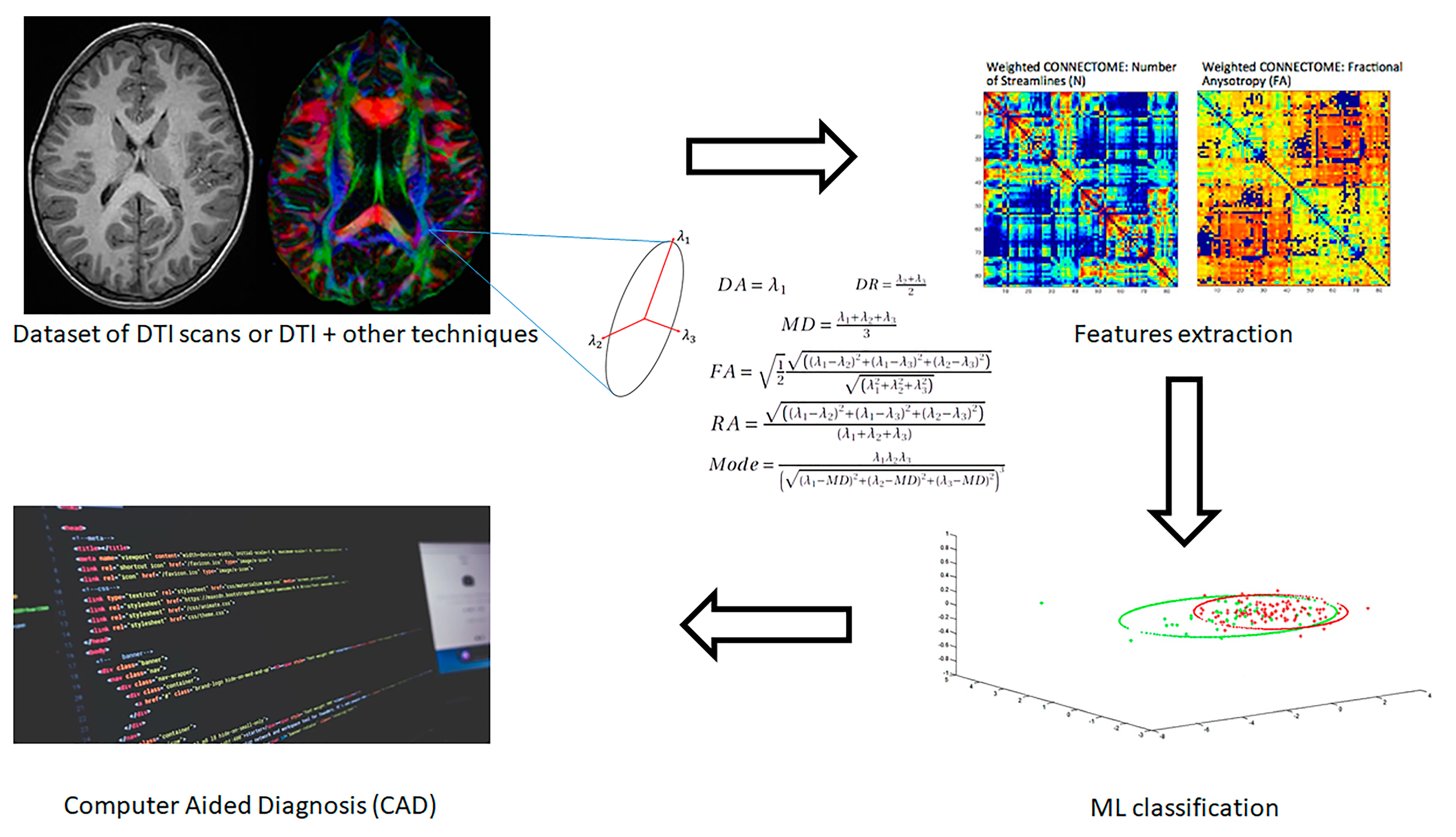
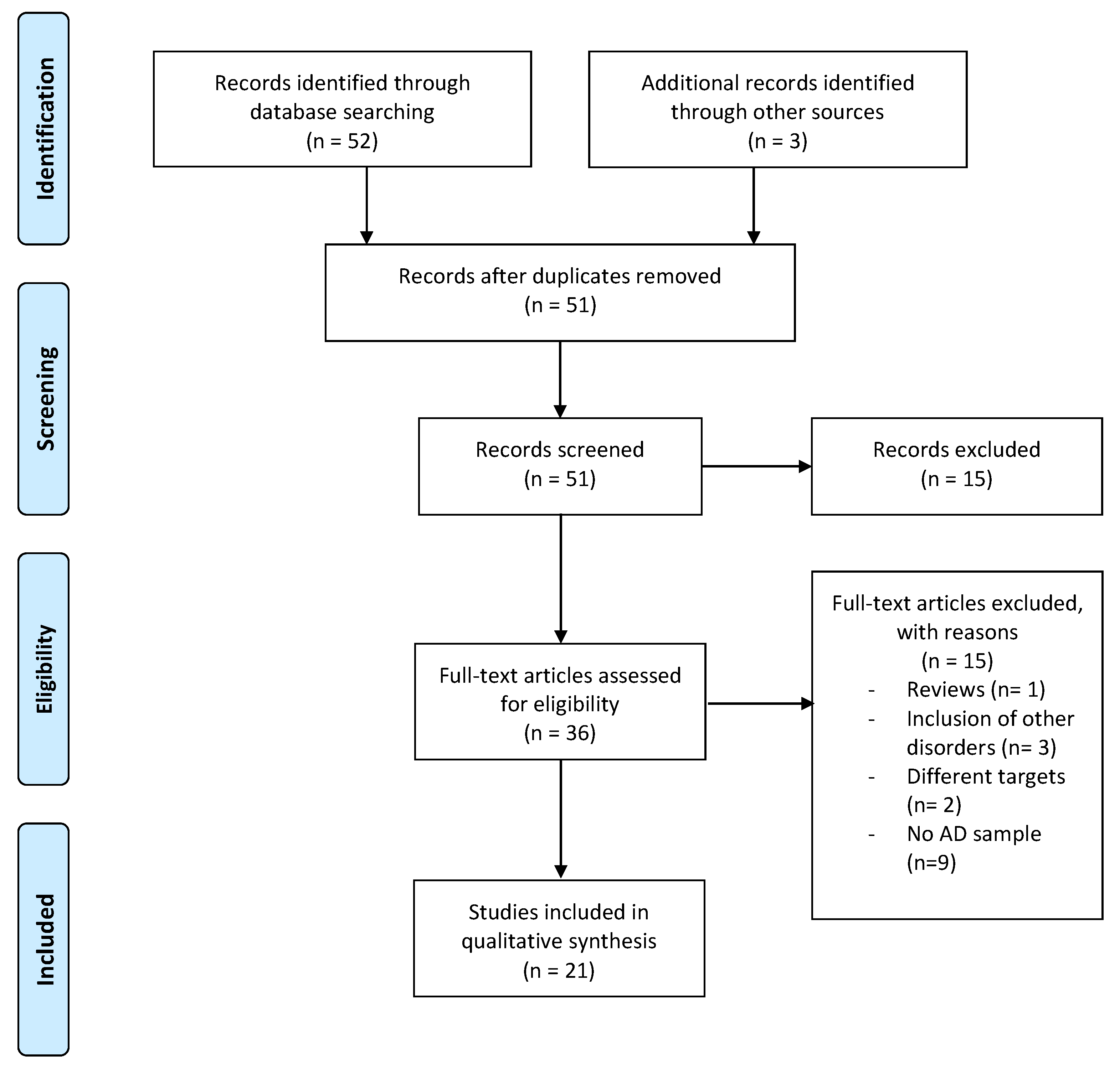
2. Materials and Methods

A systematic literature review covering the period from the year 2010 through to the year 2019 was conducted in PubMed according to the PRISMA (Preferred Reporting Items for Systematic Reviews and Meta-Analyses) guidelines [34]. Articles published before 2010 were not taken into account, due to the limited knowledge of DTI at their disposal. The search strategy was (“machine learning” OR “artificial intelligence” OR “classification”) AND “diffusion tensor imaging” AND (“alzheimer’s disease” OR alzheimer’s OR alzheimer).
To reduce a risk of bias, two authors (L.Bi. and A.B.) independently screened paper abstracts and titles and analyzed the full papers that met the inclusion criteria, as suggested by the PRISMA guidelines.
Overall, the search was limited to articles pertaining to studies that used supervised machine learning methods on data derived from DTI or from other neuroimaging techniques combined with DTI. Moreover, we included only studies that classified AD patients compared to healthy controls, or that also included a sample of MCI subjects. We decided to exclude articles that did not include a sample of AD but only included MCI patients and controls, since this review is mainly focused on the automatic diagnosis of AD, and since we wanted to evaluate the benefits and the issues of using DTI combined with ML methods, according to the literature so far, in a sample which is more uniquely characterized and more homogeneous compared with MCI group. This search led to 51 articles, 36 of which were selected. Among these, 15 articles were excluded: three of them were not focused on AD or MCI disorders, nine did not consider any AD sample and one systematic review and two studies did not involve DTI-based classification. From the remaining 21 articles, a consistent set of information was extracted: the neuroimaging techniques involved, the number of pathologic patients and healthy controls, the list of features, the classification algorithm(s) and the results (accuracy—ACC, sensitivity—SEN, specificity—SPE). When multiple classifiers were tested, only the performance of the one that achieved the best result are reported in Table 1 and Table 2. In Figure 1, the general procedure for data analysis and classification applied in the selected articles is represented.
In Appendix A, a comprehensive list of the acronyms and abbreviations used throughout the paper can be found, while Appendix B contains a brief description of the ML approaches mentioned in this paper.

3. Results

The 21 articles selected (Figure 2) are separated in two groups: classification considering only AD patients and healthy controls (HC) (n = 11) and classification including MCI patients (n = 10). For each article, when multiple classification approaches were tested, the best performance is reported in bold. Since some studies did not provide all the exact values of accuracy, sensitivity or specificity, these values have been deduced from plots.

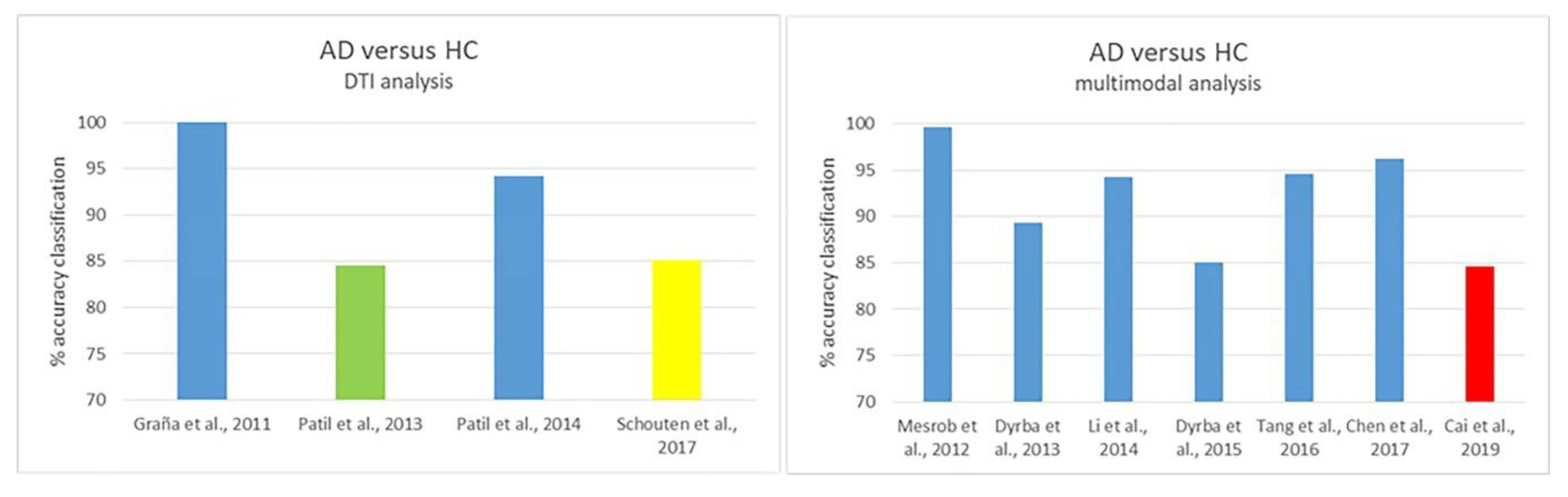
3.1. AD/HC Classification

The articles included in this review have been further classified depending on the type of neuroimaging technique used. Information extracted is showed in Table 1. Among the eleven studies of Table 1, four of them analyzed only DTI scans (DTI analysis), while the remaining seven also involved other neuroimaging modalities such as sMRI and rs-fMRI (multimodal analysis).

3.1.1. DTI Analysis

Graña et al. [35] trained an SVM using DTI measures to classify AD patients and HC. Images from DTI scans were preprocessed, in order to extract FA and MD. Different methods of cross-validation were employed, and the most accurate prediction was obtained by the leave-one-out method: with FA features, a 100% accuracy, sensitivity and specificity were achieved, while MD features achieved lower values.
Patil et al. [36] identified specific white matter regions which might represent AD markers. Classification between AD and HC was performed by the Adaptive Boosting (AdaBoost) algorithm. Considering FA measures and a set of 10 features, selected by a genetic algorithm, the accuracy, sensitivity and specificity scores were, respectively, 84.5%, 80.2% and 85.2%. If the feature set is not reduced, these values decreased due to overfitting (ACC = 75.3%), thus proving that features’ reduction improves classification accuracy by removing redundancy. It can be noticed that, considering MD in place of FA, no significant changes in accuracy were observed, suggesting that FA is an effective parameter for AD/HC classification.
Patil and Ramakrishnan, in a successive study [37], focused on the correlation between the DTI indices and the mini-mental state examination (MMSE) score. FA, MD, DR and DA measures were obtained from DTI images of AD-damaged cerebral areas and then fed singularly or along with MMSE as inputs of an SVM, decision stumps and a simple logistic. The best results were achieved by considering the feature combination of FA and MMSE score (ACC = 94.2%) with SVM. Although there was not a significant correlation between DTI indices and MMSE score, the latter improved classification accuracy for each parameter.
Schouten et al. [38] differentiated between AD and HC through four DTI measures: FA, MD, DR and DA. As a first step, voxel-wise measures (FA, MD, DR, DA) were extracted via TBSS; these voxel measures were then separately clustered with independent component analysis (ICA). Then, probabilistic tractography applied on the clustering results allowed to determine a structural connectivity network and graph measures. Using TBSS, best accuracy was reached by RD (ACC = 84.8%), closely followed by the other DTI measures. ICA reached an accuracy of 85.1% with FA, while other performance scores were not dissimilar to those of TBSS. The ICA method allowed a significant reduction of features, while structural connectivity-based classification showed best results on the connectivity graph (ACC = 85.0) compared to other measures. Lastly, the Sparse Group Lasso (SGL) was used to assess the performance of parameters’ combination: although reaching good classification accuracy, the best values were achieved by single parameters. Nevertheless, SGL shows that the most important contribution is given by TBSS and ICA’s measures, connectivity graph and strength parameters. This finding suggests that DTI and graph theory provide complementary information.

3.1.2. Multimodal Analysis

Mesrob et al. [39] developed a multimodal method to classify AD and HC based on data from both DTI and structural MRI (sMRI). The model identified 73 anatomical cerebral regions of interest (ROIs) and the extraction of different parameters concerning them. Most distinctive regions for discrimination between subjects were selected using both univariate (t-test) and multivariate (SVM-based recursive feature elimination (SVM-RFE)) methods and then used to train an SVM for classification. FA and MD from DTI were considered, while gray matter concentration (GMC) was obtained from sMRI. Moreover, two multimodal parameters were used: MD/GMC and MD/FA. The best accuracy value (ACC = 99.6%) was achieved by the multimodal parameter MD/GMC on the 15 regions chosen through the multivariate feature selection method. Interestingly, the GMC parameter alone obtained higher accuracy value (76.5%) than any other accuracy obtained by other single parameters. However, classification with the multimodal parameter in the selected regions outperformed all other parameters combined.
Dyrba et al. [40], combined data originating from different kinds of scanners to classify AD patients and controls by considering FA and MD from DTI and the densities of white matter and gray matter (WMD, GMD) from sMRI. Such processed data served as the training set for an SVM and a naïve Bayes (NB) classifier. Furthermore, two different methods of cross-validation (CV) were employed: pooled CV and scanner-specific CV. Entropy-based information gain (IG) criterion, which allows to identify the more useful features for data separation, was used for feature selection. As expected, the SVM was more accurate than the NB classifier: best results were achieved by SVM using a pooled CV method on GMD data, with an accuracy of 89.3%. Interestingly, DTI data yielded inferior accuracy compared to GMD data.
Li et al. [41], combined DTI and sMRI indices to assess their discriminatory power in AD/HC classification. FA was measured from both tract- and voxel-based DTI, while gray matter volume (GMV) was obtained from sMRI. The best classification outcome resulted in the combination of tract-based FA and GMV (ACC = 94.3%). Considering only DTI indices, it was observed that tract-based FA yielded better accuracy than voxel-based FA.
Dyrba et al. [42] compared data derived from three different neuroimaging techniques: DTI, sMRI and resting-state functional MRI (rs-fMRI). The selected diffusion indexes were FA, MD and mode of anisotropy (MO). GMV was obtained from sMRI, while two parameters were extracted from rs-fMRI: “local clustering coefficient” and “shortest path length”. Both single and multimodal parameters were used to train and test an SVM. A multiple kernel SVM (MK-SVM) was also tested, which allows for the combination of different imaging modalities. High accuracy values were reached using singular DTI indices (ACC= 85.0%) and GMV alone (ACC= 81.0%) as inputs for SVM, while for multimodal analysis, accuracy was 85.0% combining DTI measures and GMV. The multimodal results did not differ significantly from the results of the single modalities. In addition, the MK-SVM did not improve the results.
Chen et al. [43], assumed that combining DTI and DKI (diffusion kurtosis imaging) data could improve Alzheimer’s detection compared to single modalities. Diffusion indices (FA, MD, DA, DR) were measured from both DTI and DKI, while kurtosis indices (mean kurtosis—MK, axial kurtosis—AK, radial kurtosis—RK) were obtained from DKI. Two different methods of features selection were employed: SVM-RFE and correlation coefficients with MMSE score (CORR-MMSE). SVM-RFE ranking led to high scores in the occipital white matter, whereas the scores from CORR-MMSE ranking selected the splenium of the corpus callosum and the posterior limb of the internal capsule, which were omitted in the scoring of diffusivity indices. According to these results, different regions are more predictive of the condition in different parametric maps and this presented a different sensitivity effect of matrices in pathological detection. The results show that DKI-diffusion indices (Diff-DKI) yielded a better performance than DTI-diffusion indices (Diff-DTI) (ACC = 92.4% vs. ACC = 81.1%). Moreover, the highest performance (ACC = 96.2%) resulted from the combination of kurtosis and diffusion indices from DKI (ALL-DKI), highlighting that kurtosis provided additional information in the detection of abnormalities.
Cai et al. [44] selected 330 participants from the ADNI (Alzheimer’s Disease Neuroimaging Initiative) database and developed a classifier based on structural brain network modeling through the rich-club hierarchical network paradigm. Both the Automated Anatomical Labeling (AAL) and the Harvard-Oxford Atlas (HOA) were considered for the structural networks’ construction, performed on DTI and b0 (sMRI) images, aligned with the PANDA pipeline tool, for each individual included in the study. The classification between AD and HC was performed through linear discriminant analysis (LDA) on the following topologic parameters extracted from the resulting structural brain networks: “betweenness centrality (BC)” and “connection strength”. The classification accuracy of both BC and connections strength was compared with common measures in AD diagnosis: hippocampal volume and MMSE. The study findings reported significant difference in BC and connection strength between AD and controls for some brain regions, which were specific to each atlas (AAL or HOA). These relevant connections were considered as classification features to distinguish AD from controls. The best results were obtained using the AAL atlas, which achieved the best outcome in particular (ACC = 84.62%), with BC applied to the left putamen and left precuneus.
Tang et al. [45] closely examined the feasibility of AD/HC classification through volumetric, morphometric and DTI-based features specifically extracted from hippocampus and amygdala. T1 sMRI images of the participants were segmented with a two-level diffeomorphic multi-atlas likelihood-fusion algorithm and the help of an expert neuroanatomist, in order to calculate the volume of hippocampus and amygdala. The T1 images were also 3D segmented, creating triangulated surfaces of the regions of interest, and through large deformation diffeomorphic metric mapping (LDDMM), shrinking or expansion of local surface vertices, in relation to the adequate template, was estimated. DTI images were processed and segmented to obtain FA and MD values of hippocampus and amygdala. The feature set thus included volumetric measures, DTI indices and the deformation degree at each vertex of the modeled surfaces. Given the high number of vertices (over 1200), feature reduction through principal component analysis (PCA, selecting 95% of variance) and t-test was explored. Classification was performed with both LDA and SVM, validated through leave-one-out cross-validation, with SVM achieving the best results, reaching an accuracy of 94.6% for the best-case scenario with the most significative feature set, for 37 total subjects. Even though the feature reduction process significantly improved the performance of the LDA classifier, while not substantially affecting SVM, the SVM classifier still outperformed the LDA. Given the complexity of results of this study in Table 1, we only reported the performance for the right hippocampus using SVM, for which the best performance was obtained, showing how the results change according to the combination of the image modalities used.

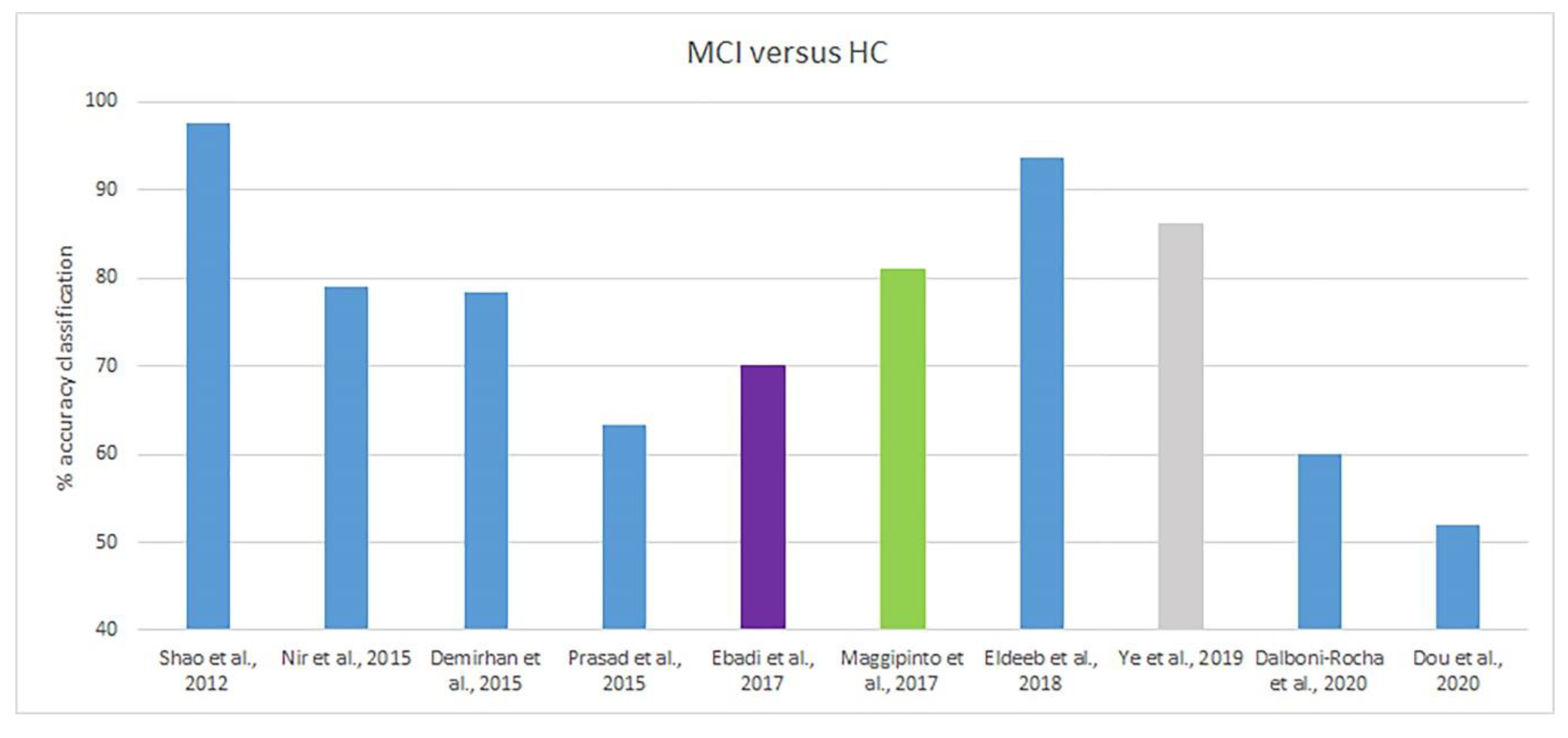
3.2. AD/MCI/HC Classification

In Table 2, ten articles that include MCI classification are summarized. All these studies employ only DTI analysis.
Shao et al. [46] proposed individual structural connectivity networks (ISCNs) to distinguish predementia and AD from healthy aging, in individual scans. For each connection, three attributes were calculated: fiber density (FD), the mean value of FA and mean value of MD across all voxels for all connection fibers. Once the structure of ISCNs was identified, three classifiers, namely, SVM, k-nearest neighbor (k-NN), NB were trained to classify subjects based on selected connections. Among the considered ML models, SVM yielded better accuracy. Patients with AD were distinguished from healthy control subjects with an accuracy of 100% using FD and MD, while patients with MCI were distinguished from healthy controls with an accuracy higher than 90%. This result is in line with previous findings of widely distributed FA decreases and MD increases in MCI. Furthermore, groups of MCI and AD patients were separated with an accuracy of about 85%, suggesting that ISCN alterations increase during the course of AD. These study findings suggested that ISCNs may have the potential of providing an imaging- and white matter-based biomarker for distinguishing between healthy subjects, aging subjects and patients with very early AD.
Nir et al. [47] investigated white matter integrity via a novel tract clustering and registration method that combines the strengths of voxel-wise and tractography-based methods, offering a compact representation of fiber bundles. In the proposed method, maximum density paths (MDP) was applied to whole-brain tractography. Differences in WM microstructure were determined by comparing FA and MD along each MDP. Significant MD and FA differences between AD patients and HC subjects were found, as well as MD differences between HC and late MCI subjects. Significant associations between FA, MD and MDP measures and cognitive deficits, as measured by MMSE scores, were also observed across all subjects. To discern between HC and AD groups, FA and MD values were tested along all the mean MDP points (1080 points). The subset of significant FA points (FAFDR CvA = 214 points) and the subset of significant MD points (MDFDR CvA = 641 points) was further tested: to distinguish between HC and MCI, all the MD values along all the MDP points (1080 points) were used, as well as the subset of significant MD points (MDFDR CvL = 12 points). Only MD measures were sensitive enough to detect MCI differences and revealed more profuse associations than FA in all analyses. The features interpolated along full mean MDPs were robust enough to reach high classification accuracies (~80%), so that reducing dimensionality by including only statistically significant MDP points did not dramatically increase classification accuracy (~85%).
Demirhan et al. [48] combined FA and MD measures from DTI to train an SVM classifier for the classification of HCs, AD and MCI patients. Good performances were reached by distinguishing AD from HC (87.8%), and MCI from HC (85.9%), while a lower value (78.4%) was obtained in separating MCI from AD subjects. Through ReliefF, an algorithm that makes it possible to identify the most discriminative voxels in white matter’s map, a best feature set consisting of 1500 elements was extracted. Selecting a subset of these features did not provide a noticeable improvement in classification accuracy if the disease was at late stages. On the other hand, the selection of specific cerebral regions considerably improved the AD/MCI and MCI/HC classification.
Prasad et al. [49] compared an ensemble of different anatomical connectivity measures using both fiber and flow connectivity methods that may help in detecting AD patients. These features were fed into a repeated, stratified 10-fold cross-validation design, using SVMs to classify controls vs. AD, controls vs. early MCI (eMCI), controls vs. late MCI (L-MCI), and eMCI vs. L-MCI. The results exhibit a significant difference in the accuracy of the various feature sets used to distinguish between the various diagnostic groups. In each of these classification problems, nine different sets of features were used: the fiber connectivity matrix, (FI(M)), the flow connectivity matrix (FL(M)), the fiber network measures (FI(N)), the flow network measures (FL(M)), combinations of these sets as FI (N+M), FL(N+M), FI(N)+FL(N), FI(M)+FL(M) and FI(N+M)+FL(N+M). All of these connectivity measures were derived simply from diffusion images. The emphasis of the study was to explore and understand which diffusion-based network measures are predictive of Alzheimer’s disease, in contrast to the optimization of classification accuracy, as in previous studies. In this way, the classification accuracy was adopted as the metric to evaluate different types of brain connectivity features, and to understand which ones may have an advantage in predicting MCI or AD insurgence.
Ebadi et al. [50] investigated the diagnostic potential of brain connectivity models regarding AD and MCI, applying graph theory to DTI measures. Graphs represented connections between different cerebral areas; once the graph measures were extracted, the best features were selected, in order to optimize the classifier’s performance and reduce overfitting. Classification was conducted through different classification methods (logistic regression, random forest, NB, k-NN and SVM) and combining their output, to improve the performance of the whole model (Ensemble). They also tested a k-best feature selection method where the features are ranked based on their power in performing the classification, and then the top K features are selected for the given estimator. Ensemble with feature selection obtained the best performance. AD patients and HC were classified with an accuracy of 80.0%, while MCI patients were separated from controls with an accuracy of 66.7%; overall, the AD/MCI ratio reached an accuracy of 76.7%.
Maggipinto et al. [51] proved the effect of feature selection bias (FSB) occurring in DTI-based AD classification, leading to an overestimation of performance metrics. FA and MD maps were extracted and registered to the same reference, and the regions corresponding to white matter were isolated through the TBSS algorithm, extracting the skeleton of white fiber tracts for each patient. Feature selection was performed via Wilcoxon rank sum test and the ReliefF algorithm both in a “nested” (unbiased) and “non-nested” way: in the former, feature selection is done after training, while in the latter it is performed before the training (i.e., only once). The classification task was accomplished by a random forest with B = 300 learning trees trained with bootstrap aggregating. Performance was assessed with 100 rounds of 5-fold cross validation. The results showed that the performance diminished using a nested approach. For example, for FA accuracy, it dropped from a maximum mean value of 87% (non-nested) to 75% (nested) in AD/HC discrimination, while for MCI/HC accuracy dropped from 81% to 59%. The same behavior was observed considering MD, where ACC decreased from 83% to 76%, and from 79% to 66% for the AD/HC and MCI/HC classification, respectively.
Eldeeb et al. [52] proposed a novel method to extract relevant markers associated with FA and MD. After preprocessing of DTI-data, FA and MD maps of regions of interest were determined using a “bag-of-words” model. This model has been used to model the hippocampus diffusivity maps patterns, through clustering the extracted hippocampus features, where the number of features is changing from one slice to another. Both the speeded up robust features (SURF) and the scale invariant feature transform (SIFT) features were extracted. With these FA and MD maps, an SVM was then trained to classify the different groups of subjects. Classification was performed for each pair of groups, and then between all of the classes, solving a multiclass problem. The best accuracies were obtained with MD map using a SIFT features descriptor and are reported as follows: 98.3% AD/HC, 93.6% MCI/HC, 92.0% AD/MCI and 89.0% multiclass.
Ye et al. [53] conducted a connectome-wide association (CWAS) study on AD, stable MCI (sMCI), MCI converting to AD (cMCI) and healthy patients selected from the ADNI database to explore the alterations in structural connectivity networks of white matter without any a priori hypothesis on pathologic alterations. Whole-brain connectomes were generated through probabilistic fiber tracking of registered T1 images and DTI scans, separated in 90 regions according to the AAL atlas. Multivariate distance matrix regression (MDMR) paired with the delta method were applied to assess the variation of distance in connectivity patterns, highlighting the brain regions that displayed greater differences between the study groups. The discriminatory power of the connectivity features isolated by the MDMR analysis was tested by comparing the classification performance obtained with them against the whole-brain connectivity features, using a partial least squares discrimination analysis (PLS-DA) classifier with five-fold cross-validation on 161 subjects. For cMCI/HC classification, considering MDMR-selected features over whole-brain ones, the SEN score increased from 54.7% to 71.3%, while SPEC decreased from 85.0% to 79.3%; regarding AD/HC classification, SEN went from 71.9% to 67.0%, while SPEC grew from 70.1% to 76.2%.
Dalboni da Rocha et al. [54] classified AD, MCI and HC through an SVM applied to the patients’ FA maps obtained through DTI, focusing on brain areas frequently associated with AD abnormalities. The analysis was repeated for the whole-brain and in specific brain areas both with and without a feature selection stage, based on the Fisher Score. As expected, results obtained without feature selection were lower. Among all the considered brain areas, two of them showed greater discriminatory power (consistently lower FA) between AD and HC: the bilateral cingulum in the hippocampal formation and the parahippocampal gyrus, in accordance with previous studies on AD indicating parahippocampal white matter modifications. Repeating the analysis of both regions by requiring the voxels to have a minimum Fisher Score (0.4/0.8) led to a maximum ACC of 93% in AD/HC classification considering the cingulum in the hippocampal formation and 90% for the parahippocampal gyrus. However, MCI/HC classification showed lower accuracy, in some cases close to chance level, possibly due to the inability to assess FA on a submillimeter scale.
Dou et al. [55] evaluated the integrity of whole-brain WM structure using automated fiber quantification (AFQ) for AD, amnestic MCI and healthy patients. The corrected, b0-aligned DTI images of the patients were processed with the AFQ toolkit in order to identify 20 major fiber tracts that have been shown to be relevant in AD progression, first by estimating the fiber tractography and then by segmenting the fiber tracts of interest. The FA, MD, DR, DA of each point was determined. Three classifiers were tested on a set of 1440 features per patient: SVM, LDA and extreme gradient boosting (XGB). Performance was evaluated both with 10-fold cross-validation and leave-one-out cross-validation. The results of this study summarized in Table 2 refer to SVM with leave-one-out cross validation for which the best results were obtained. Patients were divided into a discovery dataset and a replicated dataset and the statistical analysis, model learning and validation was repeated for both databases, obtaining agreeing results: ACC = 82.56–83.72% for AD/HC classification, 77.78%–82.28% for AD/aMCI classification and 52.02%–51.25% for aMCI/HC classification.

4. Discussion

In this review article, we identified twenty-two studies applying ML techniques for the classification of AD based on DTI imaging data, used alone or in combination with other imaging techniques. Some of the reviewed studies only differentiated between AD patients and healthy controls, while others also included a group of MCI patients for the identification and differentiation of the prodromal stage of the disease.
To the best of our knowledge, this is the first study that systematically reviewed classification approaches in AD with a focus on DTI. The attention to this specific technique is due to the fact that DTI is sensitive to microstructural white matter changes that are not visible with conventional volumetric techniques, and thus may contribute to the search for early biomarkers of the disease [56].
Studies discussed in this review have highlighted the role of DTI data as biomarkers of AD and MCI. Combining the application of ML approach with features extracted from DTI scans can provide a customized diagnosis for the early identification of AD, MCI and healthy subjects. Importantly, one of the great advantages of applying classification algorithms on neuroimaging data is the potential use for detecting AD at the prodromal stages, even well before clinical manifestation [57], which would have potential application in routine clinical settings in the future. In particular, the early detection of MCI is fundamental, since existing AD therapies show better results if the disease is still at earlier stages.
As regards the binary classification between AD and HC, very high performance in terms of accuracy (>90%) was achieved by several studies ([35,37,39,41,43,46,52]), among which, two even obtained 100% accuracy ([35,46]) (Figure 3). However, it should be noted that the sample size of these studies, in particular of the ones obtaining an accuracy of 100%, is quite limited (15–35 subjects per group), thus, the model could have been overfitted and could lack generalizability.
Studies reported in this review show evidence that automated DTI-based classifications of both MCI/HC and MCI/AD provide considerably inferior results than AD/HC separation (accuracy: ~80%). Only two studies obtained an accuracy higher than 90% [46,52], but also in this case, the limited sample size needs to be considered as a potential bias (Figure 4). Lower accuracy in these classifications is probably due to less marked differences between the features extracted. In addition, it is worth mentioning that, also from a clinical point of view, there is less confidence in the underlying pathology in MCI patients. Indeed, MCI itself is an heterogenous group, which is not always screened for primarily amnestic type or amyloid biomarkers that would increase the probability of prodromal AD.
Only one work [52] investigated the ternary problem: AD vs. MCI vs. HC and reached a good performance (accuracy = 89%). Thus, from this study, it seems that the integration of DTI with ML can be a variable instrument for the AD vs. MCI vs. HC classification also in clinical practice.
Interestingly, one study [49] also compared early MCI (eMCI) vs. late MCI (L-MCI), obtaining a quite low accuracy (63.4%). Thus, the problem of detecting subtle differences between subgroups needs to be further investigated.
Importantly, the reviewed studies differed by several factors including the sample sizes, the imaging analysis approach (i.e., voxel-based vs. tract-based), different features extracted, different feature selection methods and classification approaches. For this reason, it is difficult to quantitatively compare the different studies, while a qualitative analysis of the results can be performed.
Concerning the classification approach, it can be observed that SVM was the most frequently adopted method both for the classification of only AD [35,37,39,40,41,42,43,45] or also MCI [46,47,48,49,52,54,55] classification (Figure 3 and Figure 4). Linear discriminant analysis [44,45,55] or naïve Bayes [40,46] were also sometimes used in AD classification. Other less common classification algorithms retrieved used AdaBoost [36], extreme gradient boosting [55], Logistic elastic net regression [38], k-NN [46], Ensemble classification [50], random forest [51] and PLS-DA [53] (Figure 3 and Figure 4).
Few studies have compared different classification approaches [40,45,46,55], all of them finding that SMV outperformed the other classifiers. However, in future studies, it would be useful to perform a more extensive comparison of the performance of diverse classification algorithms.
Another important factor that influences the performance concerns the extracted features. The first important distinction is between studies which computed voxel-based or ROI-based features (i.e., [35,36,37]) vs. studies relying on tract-based features (i.e., [38,49]). In the first case, diffusion features are computed in each voxel, or in specific ROIs, of the whole-brain, while in the second method, white matter fiber tracts are estimated and for each tract, the mean value of the desired diffusion feature is calculated. Then, while most of the studies computed quite common and simple diffusion features like fractional anisotropy, mean diffusivity, betweenness centrality, radial or axial diffusivity and connectivity strength (i.e., [35,37,44,51]), few studies extracted more complex features [38,49].
Most of these studies showed that FA represents the best diffusion feature for classification models and provides valuable information to distinguish between AD and healthy subjects [35,37,38,51], while others obtained better results using other features like MD [47,52]. Concerning MCI vs. HC classification, some studies [46,47,49,52] reached better performances using mean diffusivity and fiber density as features.
In one study [41], the performances using voxel- and tract-based features were compared. According to the result of this study, tract features seem to perform better in differentiating between AD and HC. This could be due to the fact that the clustering of voxel in the tracts reduces dimensionality by grouping voxels with similar anatomic and functional characteristics.
In addition, two studies [37,44] found that clinical parameters, such as MMSE score, can also improve classification performances, meaning that the inclusion of other types of features, like clinical scores, can improve the performance.
In addition to classification and feature extraction, feature selection is also important for identifying discriminating features. The selection of appropriate features not only removes the non-informative signal, but also reduces the computational time involved in classification. The two most adopted methods for feature selection are biologically informed and automated feature selection methods. The former relies on prior biological knowledge about the discriminating ability of certain regions, generally obtained from existing literature, whereas the latter selects features based on general data characteristics, without prior knowledge.
The automated methods applied in the reviewed studies included genetic algorithm [36], t-test [39,45], recursive feature elimination [39,43], PCA [45], Wilcoxon rank sum test [51], ReliefF algorithm [48,51], multivariate distance matrix regression [53], false discovery rate [47] and k-best method [50]. Although it is difficult to say which is the best feature selection algorithm, since a comparison study is missing and several studies differentiate for multiple factors, it is evident from all these studies that selecting the most discriminant features improves the performance of the classifier by eliminating redundant or less useful features from the dataset. In particular, [51] shows that a feature selection which is blind to the t-test, leads to overoptimistic results (10% up to 30% relative increase in area under curve (AUC)).
Some studies applied a biologically informed selection method and focus only on regions, which are known to be compromised in AD, in particular hippocampus [44,45], parahippocampal gyrus and hippocampal cingulum [54] or amygdala [45]. Indeed, the hippocampus and the amygdala are among the anatomical structures of particular interest to the study of AD, mainly because of their active involvement in memory [58]. Both the global volume and the local shape of the hippocampus and the amygdala have been found to be compromised in AD [59,60]. The performance obtained by these studies are comparable to those obtained using automated methods. In particular, diffusion features from the right hippocampus [38,45] or from the parahippocampal gyrus [54] provided the best results in discriminating between AD/HC or AD/MCI. Indeed, it has previously been suggested that automated feature selection will not improve classification accuracy as compared to biologically informed feature selection, driven by prior biological knowledge of regions typically affected by AD, such as the hippocampus, amygdala, thalamus and caudate [61]. Notably, in the classification MCI/HC, whole-brain analysis performed better in [54], possibly due to the more subtle and sparse alterations in the prodromal stage of the disease.
The last important point to be considered when discussing the reviewed studies concerns the application of unimodal versus multimodal images. For AD/HC classification, five studies integrated DTI with sMRI [39,40,41,44,45], while only one also added fMRI [42]. One study also combined DTI with a more novel technique, which is DKI [43]. Notably, none of those studies applied a multimodal approach for the classification of MCI compared with AD.
All but one study [40] found that the results obtained using DTI measures outperformed those obtained with volumetric images. The contradictory results in [40] could be due to the advanced stage of the patient included in the study, so that the brain volume was highly compromised with cortical atrophy. Another possible explanation for this contradictory result could be represented by the multi-centric nature of the study. Indeed, it has been pointed out that DTI is more affected by site effects due to differences in acquisition parameters than volume measures [62]. For this reason, combining images of different sites could have mostly compromised the classification accuracy for DTI images.
In addition, most of these studies found that the combination of multimodal features outperformed the results obtained by using one single technique. Indeed, DTI-based features serve as a complementary tool to volume-based features, as the two imaging techniques reflect tissue changes associated with AD that correspond to pathological evidences in the gray matter and white matter, respectively. Thus, from the results of this review, it seems that combining several neuroimaging modalities is promising for further understanding the underlying disease mechanisms. However, it must be noted that [42] found that combining parameters from different neuroimaging modalities does not significantly improve AD/HC separation. Thus, future studies need to assess whether multimodal imaging, including functional (or metabolic) imaging methods, provides additional diagnostic accuracy for the classification of AD clinical labels, which could only be obtained from pathology.
In addition to the above-mentioned future lines of research, including the testing and fair comparison of different classifier and different feature extraction/selection approaches and a more systematic evaluation of the benefits of multimodal imaging compared with unimodal one, other future directions can be suggested. At first, it would be important to include larger samples of subjects since most of the reviewed study deals with quite low study groups. Larger samples from different sites, together with better pooling analysis methods, may improve the statistical power of the analysis, allowing to obtain more reliable information [63].
Then, future works should be more focused on the integration of heterogenous data sources, since promising results were obtained so far in this direction. Such data should importantly include physiological and functional parameters that can aid in constructing diagnostic tools with higher sensitivity and specificity, for more effective analysis of brain diseases [8]. Moreover, other miscellaneous data than neuroimaging could improve the classification of AD, including cognitive measures, risk factors associated with AD or cerebrospinal fluid measures [64].
Another important line of future direction consists in the implementation of longitudinal studies, which include different stages of AD for a better understanding of the progression of the disease, from the earliest to the most advanced stages. Indeed, a better understanding of the progression of neuronal deterioration and its correlation with psychological symptoms may help setting up new tailored treatments, such as real-time neurofeedback [65] and brain-computer interface training [66].
Finally, the application of deep learning methods and in their comparison with ML approaches should be better investigated in the future. With respect to conventional ML methods, deep learning algorithms require little or no image pre-processing, and can automatically infer an optimal representation of the data from the raw images without requiring prior feature selection, thus resulting in a more objective and less biased process [67]. Few papers on the application of deep learning approaches, and in particular convolutional neural networks, in the classification or prediction of AD using DTI imaging data have been recently published achieving good results [68,69]. More comprehensive studies are needed to evaluate the advantages of these methods compared with more traditional approaches.

5. Conclusions

To summarize, the results of this review showed that ML algorithms can be successfully applied to DTI or multimodal imaging data to deepen the current understanding of structural and functional connectivity mechanisms of AD and MCI, representing one of the ultimate goals of future AD-related research.
According to existing studies, the classification between AD and HC performs better than that between AD and MCI or MCI and HC, probably due to the less advanced study concerning MCI and to the heterogeneity of this group. Support vector machine appears to outperform the other classifiers, although in this domain other approaches (i.e., random forest) are promising. Regarding selected features, FA provided the most powerful results in AD/HC classification, possibly due to the high disruption of WM integrity, while in the detection of MCI, other features could be more reliable, in particular MD. Focusing on specific ROIs, in particular the hippocampus and the amygdala, which are known to be compromised in AD, might not decrease the performance compared with a whole-brain analysis, at least in the classification between AD and HC. Multimodal approaches that look for patterns of neurodegeneration across different kinds of bioimages are gaining increasing attention and seem to be promising for a better classification of AD or MCI. Multimodal imaging approaches, MCI-biomarkers, characterization of different stages of the disease, testing and comparing different types of classifiers, including deep learning algorithms, feature selection algorithms and bigger sample sizes, are important strategies that are likely to be emphasized in future studies.

Author Contributions

Conceptualization, L.B. (Lucia Billeci) and A.T.; methodology, A.B.; data curation, A.B., L.B. (Lorenzo Bachi); writing—original draft preparation, A.B.; writing—review and editing, L.B. (Lucia Billeci), L.B. (Lorenzo Bachi), A.T.; supervision, L.B. (Lucia Billeci). All authors have read and agreed to the published version of the manuscript.

Funding

This research received no external funding.

Conflicts of Interest

The authors declare no conflict of interest.

Appendix A

List of Acronyms and Abbreviations

AALAutomated Anatomical Labeling atlas
ACCAccuracy
ADAlzheimer’s disease
ADNIAlzheimer’s Disease Neuroimaging Initiative
AFQAutomated fiber quantification
AKAxial kurtosis
AdaBoostAdaptive boosting
ALL-DKICombination of kurtosis and diffusion indices from DKI
BCBetweenness centrality
CADComputer-aided diagnosis
cMCIMCI patients that eventually converts to AD
CORR-MMSECorrelation coefficient with the MMSE score
CSFCerebrospinal fluid
CVCross-validation
CWASConnectome-wide association
DAAxial diffusivity
Diff-DKIDKI diffusion indices
Diff-DTIDTI diffusion indices
DKIDiffusion kurtosis imaging
DRRadial diffusivity
DTIDiffusion tensor imaging
eMCIEarly MCI patient
FAFractional anisotropy
FDFiber density
GMCGrey matter concentration
GMDGrey matter density
GMVGrey matter volume
HCHealthy control patient
HOAHarvard-Oxford atlas
ICAIndependent component analysis
IGInformation gain
ISCNIndividual structural connectivity network
k-NNk-nearest neighbors algorithm
LDALinear discriminant analysis
LDDMMLarge deformation diffeomorphic metric mapping
L-MCILate MCI patient
MCIMild cognitive impairment
MDMean diffusivity
MDMRMultivariate distance matrix regression
MDPMaximum density path
MKMean kurtosis
MK-SVMMultiple-kernel SVM
MLMachine learning
MMSEMini-mental state examination
MOMode of anisotropy
MRIMagnetic resonance imaging
NBNaïve Bayes classifier
PCAPrincipal component analysis
PETPositron mission tomography
PLS-DAPartial least squares discrimination analysis
PRISMAPreferred Reporting Items for Systematic Reviews and Meta-Analyses
RARelative anisotropy
rs-fMRIResting-state functional MRI
ROIRegion of interest
RKRadial kurtosis
SENSensitivity
SGLSparse group lasso
SIFTScale invariant feature transform
sMRIStructural MRI
SPESpecificity
SURFSpeed up robust features
SVMSupport vector machine
SVM-RFESVM-based feature recursive elimination
TBSSTract-based special statistics
WMWhite matter
WMDWhite matter density
XGBExtreme gradient boosting

Appendix B

Appendix B.1. Machine Learning Overview

Machine learning (ML) is a broad term referring to an ensemble of computer algorithms that adapt their output through experience to match a desired outcome. Generally, an ML algorithm returns an output value determined by its input variables, called features, in order to refine the aptness of the computed output the program first learns on a training dataset, while evaluation of its performance is done on one or more validation datasets. The size of the data involved in both steps is crucial, as small samples could lead to unreliable results. ML models are most often grouped into three categories, depending on the nature of the learning process: in supervised learning, the program learns on a labelled dataset where the desired outcome is known, adjusting its output to replicate as best as possible the desired one; in unsupervised learning, the data is not labelled and the algorithm looks for similarities in the inputs by modeling their probability densities, highlighting the standing relations between them; in reinforcement learning, the algorithm discovers the desired outcome in a process of trial and error, and adapts its output to maximize the correct decisions that lead to it. The machine learning aspects of this review specifically concern one of the four kinds of learning problems, classification, where the output belongs to a discrete range (AD, HC and/or MCI) and with a supervised learning process. Consequently, these ML models are classifiers, i.e., objects that assign each feature vector x (a patient) to one of the c classes or groups. A brief description of each method mentioned in this paper follows. For additional background, see [70,71,72].

Appendix B.2. Support Vector Machine

The support vector machine (SVM) is a supervised, non-probabilistic linear classifier, meaning that it can learn to discriminate data belonging to two classes by searching for the linear boundary (called hyperplane) that maximizes the margin between the two known classes. If the input is an array x consisting of n features, meaning it is a point in a n-dimensional space, the SVM method finds a linear surface of dimension n-1 that divides the two clouds of n-dimensional points belonging to the two classes. That is, optimizing the hyperplane parameters in order to maximize its distance from the closest point, which is a problem that can be reduced to minimization of a quadratic error function. Although in its simplest definition SVM is a linear classifier, by employing the nonlinear kernel trick nonlinear classification can be performed. Moreover, the model can be adjusted if the two classes are not clearly separated in the n-dimensional space by relaxing the hard margin constraint in favor of a soft margin; SVM can also be adapted to resolve multiclass problems in various ways, generally by combining a bank of SVM classifiers.

Appendix B.3. Logistic Regression

Logistic regression, even if called “regression”, is actually a classification model where the relationship between the features and the log-odds (the logarithm of the odds ratio) of the c classes is assumed to be linear. In other words, the posterior probability of each class is a logistic sigmoid function acting on a linear combination of the feature vector. The n parameters of the linear function are estimated for each class, so that for each datapoint x (consisting of n features), a score corresponding to each class is computed; the observation is then assigned to the class presenting the highest score. The parameters of the logistic regression can be determined by maximizing the log-likelihood of the data with a numerical optimization algorithm, typically with regularization of the coefficients (Maximum A Posteriori (MAP) estimation), such as the ridge regression (L2 penalty), the lasso regression (L1 penalty) or the elastic net regression (L1+L2 penalty). Regularization helps prevent excessive overfitting, reducing estimator variance whilst introducing a small bias. This model is usually formulated for a two-class problem, but can be extended to an arbitrary number of classes.

Appendix B.4. Naïve Bayes Classifier

The naïve Bayes classifier refers to a simple, yet robust family of models based on the assumption that the features x are independent. This assumption allows the posterior probability distribution for each class to depend merely on the product of n one-dimensional likelihoods, thus, not requiring estimation of conditional distributions. Parameters are learned with likelihood maximization, estimating the one-dimensional densities for each class and feature, which can be done in various ways, depending on the statistical hypotheses made on the data (the naïve Bayes event model). Usually, classification of data is done by choosing the most probable outcome, i.e., the class that exhibits the higher posterior probability for the observation.

Appendix B.5. Linear Discriminant Analysis

Linear discriminant analysis (LDA), derived from Fisher’s discriminant analysis, is a classifier based on dimensionality reduction. The n-dimensional feature space is projected into one dimension with the weight array w : y = w T x . Each class is supposed to be distributed as a multivariate Gaussian, with all the covariance matrixes of the said class densities assumed to be equal (without this last assumption, the resulting model is the quadratic discriminant analysis). The log-odds of the classes posterior probability is then a linear function of x , and the decision boundary between any two classes is linear, resulting in a hyperplane in the feature space separating each pair of groups. Classification occurs by defining the thresholds over which the new data is assigned to one group instead of the others, in the projected one-dimensional space. Considering two classes 0 and 1, if w T x > c x will be assigned to class 1, otherwise to class 0. Thus, learning for this model consists in defining the direction of projection that maximizes separation between the classes w and the decision threshold c by estimating the parameters of the multivariate of the classes’ Gaussian distribution. Multiclass tasks can be performed either by combining several discriminants (one-versus-the-rest, one-versus-one) or by considering a single classifier with c linear discriminant functions.

Appendix B.6. Partial Least Squares Discriminant Analysis

Partial least squares discriminant analysis (PLS-DA) is a variant of the partial least squares regression, where the dependent variable y is converted to a categorical field. In a manner not dissimilar to principal component regression, partial least squares regression finds a set of linear combination of the inputs, selecting a subset of the components as regressors, but considering both y and x for the projection into component space. This algorithm finds the latent variables with the maximum covariance with the y variable, instead of seeking directions that explain only the most variance. Considering all available directions would correspond to a conventional least square estimate, while selecting only a subset of them leads to a reduced regression with lower chances of overfitting. The conversion of the continuous value of y into its corresponding categorical value (i.e., turning a regressor into a classifier) can be done by comparing, for each new observation x , the c class values resulting from the PLS regression: the observation is then assigned to the class that showed the highest probability.

Appendix B.7. K-Nearest Neighbors

The nearest neighbor family of classifiers process new observations x depending on the outcome of the closest datapoints. On its most elementary form, the k-nearest neighbors (k-NN) classifier assigns the data x to the most popular class among its k neighbors, where k is a user-defined parameter. Distance can be determined with various metrics, the most common one being the Euclidean distance. Several versions of supervised k-NN exists, where the object of the learning process is usually the definition of the metric that better sorts the training inputs in their respective groups. This means finding the matrix M which, placed in d ( x i , x j ) = ( x i x j ) T M ( x i x j ) minimizes the classification error.

Appendix B.8. Random Forest

The random forest is a regression and classification technique based on bagging (bootstrap aggregating), by training a large ensemble of decision trees with low correlation between them, which are then averaged. A decision tree, often represented in their flowchart structure, is a model consisting of subsequent binary splits of the input space. A tree consists of its root, the first split; its branches, the next consecutive splits; the leaves, representing the predicted value (whether continuous or categorical). Building a tree corresponds to partitioning the input space in squares with lines that are parallel to coordinate axes. In a decision tree, leaning (growing) means deciding, at each node, the splitting threshold for the n-th input feature, which can be done by exhaustive research, minimizing an error function: for classification, two common measures are cross-entropy and the Gini index. After a sufficiently large tree is built it gets pruned, removing some of its branches by balancing the error function and a measure of model complexity (cost-complexity pruning). In a random forest, several trees are built, each time selecting a subset of the input variables. After the desired number of classification trees has been trained, the output classification is the result of a majority vote. By bagging the threes, instead of considering a single, larger tree, the overall variance of the model is decreased, although its bias is unchanged.

Appendix B.9. Boosting Techniques

The term boosting refers to a technique where several weak classifiers, with performance slightly above chance level, are combined to form a powerful committee, able to get very close to the target classification performance. Adaptive boosting (AdaBoost) is one of the most popular algorithms for boosting formulated for the two-class problem, where the weak classifiers are trained consequently, the performance of each one influencing the training of the next. Every one of the M training data points x is given a weight w m , initially set to 1 / M . The first weak classifier is then trained, using the data to produce a class prediction y { 1 , 1 } . The next weak classifiers are trained after the weights are updated, giving more relevance to misclassified data. When the desired number of weak classifiers has been trained, the committee is formed: each one will contribute to the class prediction through a second set of weights a j , one for each base classifier, determined by minimizing an exponential loss error function. One of the simplest forms of base learner that can be adopted is the decision stump, a single-level decision tree: the discrimination between two classes is done by comparing the features to a single threshold. Gradient boosting is a numerical development of the boosting method, often applied to decision trees. Through a differentiable loss function, the successive weak learners are trained in the gradient direction of minimal loss (gradient descent), fitting them to the negative gradient values of the chosen function. For classification, such loss function can consist in multinomial deviance, constructing at each iteration a number of trees equal to the total number of groups c, even though for binary classification a single tree for each iteration is sufficient.

References

  1. Prince, M.; Bryce, R.; Albanese, E.; Wimo, A.; Ribeiro, W.; Ferri, C.P. The global prevalence of dementia: A systematic review and metaanalysis. Alzheimers Dement. 2013, 9, 63–75. [Google Scholar] [CrossRef]
  2. Collie, A.; Maruff, P. The neuropsychology of preclinical Alzheimer’s disease and mild cognitive impairment. Neurosci. Biobehav. Rev. 2000, 24, 365–374. [Google Scholar] [CrossRef]
  3. Alzheimer’s Association. 2019 Alzheimer’s disease facts and figures. Alzheimers Dement. 2019, 15, 321–387. [Google Scholar] [CrossRef]
  4. Jack, C.R.; Wiste, H.J.; Weigand, S.D.; Therneau, T.M.; Lowe, V.J.; Knopman, D.S.; Gunter, J.L.; Senjem, M.L.; Jones, D.T.; Kantarci, K.; et al. Defining imaging biomarker cut points for brain aging and Alzheimer’s disease. Alzheimers Dement. 2017, 13, 205–216. [Google Scholar] [CrossRef] [PubMed] [Green Version]
  5. Woolf, B.P. Building Intelligent Interactive Tutors: Student-Centered Strategies for Revolutionizing E-Learning; Morgan Kaufmann: Burlington, MA, USA, 2010. [Google Scholar]
  6. Nayak, J.; Naik, B.; Behera, H.S. A Comprehensive Survey on Support Vector Machine in Data Mining Tasks: Applications & Challenges. Int. J. Database Theory Appl. 2015, 8, 169–186. [Google Scholar] [CrossRef]
  7. Frisoni, G.B.; Fox, N.; Jack, C.R.; Scheltens, P.; Thompson, P. The clinical use of structural MRI in Alzheimer disease. Nat. Rev. Neurol. 2010, 6, 67–77. [Google Scholar] [CrossRef] [Green Version]
  8. Greicius, M.D.; Srivastava, G.; Reiss, A.L.; Menon, V. Default-mode network activity distinguishes Alzheimer’s disease from healthy aging: Evidence from functional MRI. Proc. Natl. Acad. Sci. USA 2004, 101, 4637–4642. [Google Scholar] [CrossRef] [PubMed] [Green Version]
  9. Fripp, J.; Bourgeat, P.; Acosta, O.; Raniga, P.; Modat, M.; Pike, K.E.; Jones, G.; O’Keefe, G.; Masters, C.L.; Ames, D.; et al. Appearance modeling of 11C PiB PET images: Characterizing amyloid deposition in Alzheimer’s disease, mild cognitive impairment and healthy aging. NeuroImage 2008, 43, 430–439. [Google Scholar] [CrossRef] [PubMed]
  10. Cabral, C.; Silveira, M. Classification of Alzheimer’s disease from FDG-PET images using favourite class ensembles. In Proceedings of the 2013 35th Annual International Conference of the IEEE Engineering in Medicine and Biology Society (EMBC), Osaka, Japan, 3–7 July 2013; Volume 2013, pp. 2477–2480. [Google Scholar] [CrossRef]
  11. Szmuda, M.; Szmuda, T.; Springer, J.; Rogowska, M.; Sabisz, A.; Dubaniewicz, M.; Mazurkiewicz-Bełdzińska, M. Diffusion tensor tractography imaging in pediatric epilepsy—A systematic review. Neurologia i Neurochirurgia Polska 2016, 50, 1–6. [Google Scholar] [CrossRef] [PubMed] [Green Version]
  12. Arab, A.; Wojna-Pelczar, A.; Khairnar, A.; Szabo, N.; Ruda-Kucerova, J. Principles of diffusion kurtosis imaging and its role in early diagnosis of neurodegenerative disorders. Brain Res. Bull. 2018, 139, 91–98. [Google Scholar] [CrossRef] [PubMed]
  13. Billeci, L.; Calderoni, S.; Tosetti, M.; Catani, M.; Muratori, F. White matter connectivity in children with autism spectrum disorders: A tract-based spatial statistics study. BMC Neurol. 2012, 12, 148. [Google Scholar] [CrossRef] [Green Version]
  14. Le Bihan, D.; Poupon, C.; Clark, C.A.; Pappata, S.; Molko, N.; Chabriat, H. Diffusion tensor imaging: Concepts and applications. J. Magn. Reson. Imaging 2001, 13, 534–546. [Google Scholar] [CrossRef] [PubMed]
  15. Pierpaoli, C.; Jezzard, P.; Basser, P.J.; Barnett, A.; Di Chiro, G. Diffusion tensor MR imaging of the human brain. Radiology 1996, 201, 637–648. [Google Scholar] [CrossRef] [PubMed]
  16. Alexander, A.L.; Lee, J.E.; Lazar, M.; Field, A.S. Diffusion tensor imaging of the brain. Neurotherapeutics 2007, 4, 316–329. [Google Scholar] [CrossRef] [PubMed] [Green Version]
  17. Alves, G.S.; Knöchel, V.O.; Knöchel, C.; Carvalho, A.F.; Pantel, J.; Engelhardt, E.; Laks, J. Integrating Retrogenesis Theory to Alzheimer’s Disease Pathology: Insight from DTI-TBSS Investigation of the White Matter Microstructural Integrity. BioMed Res. Int. 2015, 2015, 1–11. [Google Scholar] [CrossRef]
  18. Smith, S.M.; Jenkinson, M.; Johansen-Berg, H.; Rueckert, D.; Nichols, T.E.; Mackay, C.E.; Watkins, K.E.; Ciccarelli, O.; Cader, M.Z.; Matthews, P.M.; et al. Tract-based spatial statistics: Voxelwise analysis of multi-subject diffusion data. NeuroImage 2006, 31, 1487–1505. [Google Scholar] [CrossRef]
  19. Hagmann, P.; Cammoun, L.; Gigandet, X.; Meuli, R.; Honey, C.J.; Wedeen, V.J.; Sporns, O. Mapping the Structural Core of Human Cerebral Cortex. PLoS Boil. 2008, 6, e159. [Google Scholar] [CrossRef]
  20. Xie, S.; Xiao, J.X.; Gong, G.L.; Zang, Y.-F.; Wang, Y.H.; Wu, H.K.; Jiang, X.X. Voxel-based detection of white matter abnormalities in mild Alzheimer disease. Neurology 2006, 66, 1845–1849. [Google Scholar] [CrossRef]
  21. Ringman, J.M.; O’Neill, J.; Geschwind, D.; Medina, L.D.; Apostolova, L.G.; Rodriguez, Y.; Schaffer, B.; Varpetian, A.; Tseng, B.; Ortiz, F.; et al. Diffusion tensor imaging in preclinical and presymptomatic carriers of familial Alzheimer’s disease mutations. Brain 2007, 130, 1767–1776. [Google Scholar] [CrossRef]
  22. Cherubini, A.; Péran, P.; Spoletini, I.; Di Paola, M.; Di Iulio, F.; Hagberg, G.; Sancesario, G.; Gianni, W.; Bossù, P.; Caltagirone, C.; et al. Combined Volumetry and DTI in Subcortical Structures of Mild Cognitive Impairment and Alzheimer’s Disease Patients. J. Alzheimer’s Dis. 2010, 19, 1273–1282. [Google Scholar] [CrossRef]
  23. Teipel, S.J.; Grothe, M.J.; Zhou, J.; Sepulcre, J.; Dyrba, M.; Sorg, C.; Babiloni, F. Measuring Cortical Connectivity in Alzheimer’s Disease as a Brain Neural Network Pathology: Toward Clinical Applications. J. Int. Neuropsychol. Soc. 2016, 22, 138–163. [Google Scholar] [CrossRef] [PubMed]
  24. Naggara, O.; Oppenheim, C.; Rieu, D.; Raoux, N.; Rodrigo, S.; Barba, G.D.; Meder, J.-F. Diffusion tensor imaging in early Alzheimer’s disease. Psychiatry Res. Neuroimaging 2006, 146, 243–249. [Google Scholar] [CrossRef] [PubMed]
  25. Zhang, Y.; Schuff, N.; Jahng, G.-H.; Bayne, W.; Mori, S.; Schad, L.; Mueller, S.; Du, A.-T.; Kramer, J.H.; Yaffe, K.; et al. Diffusion tensor imaging of cingulum fibers in mild cognitive impairment and Alzheimer disease. Neurology 2007, 68, 13–19. [Google Scholar] [CrossRef] [PubMed]
  26. Medina, D.; Detoledo-Morrell, L.; Urresta, F.; Gabrieli, J.D.; Moseley, M.; Fleischman, D.; Bennett, D.A.; Leurgans, S.; Turner, D.A.; Stebbins, G.T. White matter changes in mild cognitive impairment and AD: A diffusion tensor imaging study. Neurobiol. Aging 2006, 27, 663–672. [Google Scholar] [CrossRef]
  27. E Rose, S.; McMahon, K.L.; Janke, A.L.; O’Dowd, B.; De Zubicaray, G.I.; Strudwick, M.W.; Chalk, J.B. Diffusion indices on magnetic resonance imaging and neuropsychological performance in amnestic mild cognitive impairment. J. Neurol. Neurosurg. Psychiatry 2006, 77, 1122–1128. [Google Scholar] [CrossRef]
  28. Fellgiebel, A.; Dellani, P.R.; Greverus, D.; Scheurich, A.; Stoeter, P.; Müller, M.J. Predicting conversion to dementia in mild cognitive impairment by volumetric and diffusivity measurements of the hippocampus. Psychiatry Res. Neuroimaging 2006, 146, 283–287. [Google Scholar] [CrossRef]
  29. Müller, M.J.; Greverus, D.; Dellani, P.R.; Weibrich, C.; Wille, P.R.; Scheurich, A.; Stoeter, P.; Fellgiebel, A. Functional implications of hippocampal volume and diffusivity in mild cognitive impairment. NeuroImage 2005, 28, 1033–1042. [Google Scholar] [CrossRef]
  30. Müller, M.J.; Greverus, D.; Weibrich, C.; Dellani, P.R.; Scheurich, A.; Stoeter, P.; Fellgiebel, A. Diagnostic utility of hippocampal size and mean diffusivity in amnestic MCI. Neurobiol. Aging 2007, 28, 398–403. [Google Scholar] [CrossRef]
  31. Fellgiebel, A.; Müller, M.J.; Wille, P.; Dellani, P.R.; Scheurich, A.; Schmidt, L.G.; Stoeter, P. Color-coded diffusion-tensor-imaging of posterior cingulate fiber tracts in mild cognitive impairment. Neurobiol. Aging 2005, 26, 1193–1198. [Google Scholar] [CrossRef]
  32. Choo, I.H.; Lee, N.Y.; Oh, J.-S.; Lee, J.S.; Lee, N.S.; Song, I.C.; Youn, J.C.; Kim, S.G.; Kim, K.W.; Jhoo, J.H.; et al. Posterior cingulate cortex atrophy and regional cingulum disruption in mild cognitive impairment and Alzheimer’s disease. Neurobiol. Aging 2010, 31, 772–779. [Google Scholar] [CrossRef]
  33. Selnes, P.; Aarsland, D.; Bjornerud, A.; Gjerstad, L.; Wallin, A.; Hessen, E.; Reinvang, I.; Grambaite, R.; Auning, E.; Kjærvik, V.K.; et al. Diffusion Tensor Imaging Surpasses Cerebrospinal Fluid as Predictor of Cognitive Decline and Medial Temporal Lobe Atrophy in Subjective Cognitive Impairment and Mild Cognitive Impairment. J. Alzheimer’s Dis. 2013, 33, 723–736. [Google Scholar] [CrossRef] [PubMed] [Green Version]
  34. Liberati, A.; Altman, D.G.; Tetzlaff, J.; Mulrow, C.; Gøtzsche, P.C.; Ioannidis, J.P.A.; Clarke, M.; Devereaux, P.J.; Kleijnen, J.; Moher, D. The PRISMA statement for reporting systematic reviews and meta-analyses of studies that evaluate health care interventions: Explanation and elaboration. J. Clin. Epidemiol. 2009, 62, e1–e34. [Google Scholar] [CrossRef] [PubMed] [Green Version]
  35. Graña, M.; Termenon, M.; Savio, A.; González-Pinto, A.; Echeveste, J.; Perez, J.; Besga, A. Computer Aided Diagnosis system for Alzheimer Disease using brain Diffusion Tensor Imaging features selected by Pearson’s correlation. Neurosci. Lett. 2011, 502, 225–229. [Google Scholar] [CrossRef] [PubMed]
  36. Patil, R.B.; Piyush, R.; Ramakrishnan, S. Identification of brain white matter regions for diagnosis of Alzheimer using Diffusion Tensor Imaging. In Proceedings of the 2013 35th Annual International Conference of the IEEE Engineering in Medicine and Biology Society (EMBC), Osaka, Japan, 3–7 July 2013; pp. 6535–6538. [Google Scholar] [CrossRef]
  37. Patil, R.B.; Ramakrishnan, S. Analysis of sub-anatomic diffusion tensor imaging indices in white matter regions of Alzheimer with MMSE score. Comput. Methods Progr. Biomed. 2014, 117, 13–19. [Google Scholar] [CrossRef] [PubMed]
  38. Schouten, T.M.; Koini, M.; De Vos, F.; Seiler, S.; De Rooij, M.; Lechner, A.; Schmidt, R.; Heuvel, M.V.D.; Van Der Grond, J.; Rombouts, S.A. Individual classification of Alzheimer’s disease with diffusion magnetic resonance imaging. NeuroImage 2017, 152, 476–481. [Google Scholar] [CrossRef] [PubMed] [Green Version]
  39. Mesrob, L.; Sarazin, M.; Hahn-Barma, V.; De, S.L.C.; Dubois, B.; Gallinari, P.; Kinkingnéhun, S.; Mesrob, L.; Marie, S.; Valerie, H.-B.; et al. DTI and Structural MRI Classification in Alzheimer’s Disease. Adv. Mol. Imaging 2012, 2, 12–20. [Google Scholar] [CrossRef] [Green Version]
  40. Dyrba, M.; Ewers, M.; Wegrzyn, M.; Kilimann, I.; Plant, C.; Oswald, A.; Meindl, T.; Pievani, M.; Bokde, A.L.W.; Fellgiebel, A.; et al. Robust Automated Detection of Microstructural White Matter Degeneration in Alzheimer’s Disease Using Machine Learning Classification of Multicenter DTI Data. PLoS ONE 2013, 8, e64925. [Google Scholar] [CrossRef]
  41. Li, M.; Qin, Y.; Gao, F.; Zhu, W.; He, X. Discriminative analysis of multivariate features from structural MRI and diffusion tensor images. Magn. Reson. Imaging 2014, 32, 1043–1051. [Google Scholar] [CrossRef]
  42. Dyrba, M.; Grothe, M.J.; Kirste, T.; Teipel, S.J. Multimodal analysis of functional and structural disconnection in Alzheimer’s disease using multiple kernel SVM. Hum. Brain Mapp. 2015, 36, 2118–2131. [Google Scholar] [CrossRef]
  43. Chen, Y.; Sha, M.; Zhao, X.; Ma, J.; Ni, H.; Gao, W.; Ming, N. Automated detection of pathologic white matter alterations in Alzheimer’s disease using combined diffusivity and kurtosis method. Psychiatry Res. Neuroimaging 2017, 264, 35–45. [Google Scholar] [CrossRef]
  44. Cai, S.; Huang, K.; Kang, Y.; Jiang, Y.; Von Deneen, K.M.; Huang, L. Potential biomarkers for distinguishing people with Alzheimer’s disease from cognitively intact elderly based on the rich-club hierarchical structure of white matter networks. Neurosci. Res. 2019, 144, 56–66. [Google Scholar] [CrossRef] [PubMed]
  45. Tang, X.; Qin, Y.; Wu, J.; Zhang, M.; Zhu, W.; Miller, M.I. Shape and diffusion tensor imaging based integrative analysis of the hippocampus and the amygdala in Alzheimer’s disease. Magn. Reson. Imaging 2016, 34, 1087–1099. [Google Scholar] [CrossRef] [PubMed]
  46. Shao, J.; Myers, N.; Yang, Q.; Feng, J.; Plant, C.; Böhm, C.; Förstl, H.; Kurz, A.; Zimmer, C.; Meng, C.; et al. Prediction of Alzheimer’s disease using individual structural connectivity networks. Neurobiol. Aging 2012, 33, 2756–2765. [Google Scholar] [CrossRef] [PubMed] [Green Version]
  47. Nir, T.M.; Villalon-Reina, J.E.; Prasad, G.; Jahanshad, N.; Joshi, S.H.; Toga, A.W.; Bernstein, M.A.; Jack, C.R.; Weiner, M.W.; Thompson, P.; et al. Diffusion weighted imaging-based maximum density path analysis and classification of Alzheimer’s disease. Neurobiol. Aging 2015, 36, S132–S140. [Google Scholar] [CrossRef] [PubMed] [Green Version]
  48. Demirhan, A.; Nir, T.M.; Zavaliangos-Petropulu, A.; Jack, C.R.; Weiner, M.W.; Bernstein, M.A.; Thompson, P.; Jahanshad, N. Feature selection improves the accuracy of classifying Alzheimer disease using diffusion tensor images. In Proceedings of the 2015 IEEE 12th International Symposium on Biomedical Imaging (ISBI), Brooklyn, NY, USA, 16–19 April 2015; pp. 126–130. [Google Scholar] [CrossRef]
  49. Prasad, G.; Joshi, S.H.; Nir, T.M.; Toga, A.W.; Thompson, P.M.; Alzheimer’s Disease Neuroimaging Initiative (ADNI). Brain connectivity and novel network measures for Alzheimer’s disease classification. Neurobiol. Aging 2015, 36, S121–S131. [Google Scholar] [CrossRef] [PubMed] [Green Version]
  50. Ebadi, A.; Da Rocha, J.L.D.; Nagaraju, D.B.; Tovar-Moll, F.; Bramati, I.; Coutinho, G.; Sitaram, R.; Rashidi, P. Ensemble Classification of Alzheimer’s Disease and Mild Cognitive Impairment Based on Complex Graph Measures from Diffusion Tensor Images. Front. Mol. Neurosci. 2017, 11. [Google Scholar] [CrossRef] [PubMed] [Green Version]
  51. Maggipinto, T.; Bellotti, R.; Amoroso, N.; Diacono, D.; Donvito, G.; Lella, E.; Monaco, A.; Scelsi, M.A.; Tangaro, S.; Initiative, A.D.N. DTI measurements for Alzheimer’s classification. Phys. Med. Boil. 2017, 62, 2361–2375. [Google Scholar] [CrossRef] [PubMed]
  52. Eldeeb, G.W.; Zayed, N.; Yassine, I.A. Alzheimer’S Disease Classification Using Bag-Of-Words Based on Visual Pattern of Diffusion Anisotropy for DTI Imaging. In Proceedings of the 2018 40th Annual International Conference of the IEEE Engineering in Medicine and Biology Society (EMBC), Honolulu, HI, USA, 17–21 July 2018; pp. 57–60. [Google Scholar]
  53. Ye, C.; Mori, S.; Chan, P.; Ma, T. Connectome-wide network analysis of white matter connectivity in Alzheimer’s disease. NeuroImage Clin. 2019, 22, 101690. [Google Scholar] [CrossRef]
  54. Da Rocha, J.L.D.; Bramati, I.E.; Coutinho, G.; Moll, F.T.; Sitaram, R. Fractional Anisotropy changes in Parahippocampal Cingulum due to Alzheimer’s Disease. Sci. Rep. 2020, 10, 1–8. [Google Scholar] [CrossRef]
  55. Dou, X.; Yao, H.; Feng, F.; Wang, P.; Zhou, B.; Jin, D.; Yang, Z.; Li, J.; Zhao, C.; Wang, L.; et al. Characterizing white matter connectivity in Alzheimer’s disease and mild cognitive impairment: An automated fiber quantification analysis with two independent datasets. Cortex 2020, 129, 390–405. [Google Scholar] [CrossRef]
  56. Weston, P.S.; Simpson, I.J.; Ryan, N.S.; Ourselin, S.; Fox, N. Diffusion imaging changes in grey matter in Alzheimer’s disease: A potential marker of early neurodegeneration. Alzheimer’s Res. Ther. 2015, 7, 47. [Google Scholar] [CrossRef] [PubMed] [Green Version]
  57. Misra, C.; Fan, Y.; Davatzikos, C. Baseline and longitudinal patterns of brain atrophy in MCI patients, and their use in prediction of short-term conversion to AD: Results from ADNI. NeuroImage 2009, 44, 1415–1422. [Google Scholar] [CrossRef] [PubMed] [Green Version]
  58. A Phelps, E.; Phelps, E. Human emotion and memory: Interactions of the amygdala and hippocampal complex. Curr. Opin. Neurobiol. 2004, 14, 198–202. [Google Scholar] [CrossRef] [PubMed]
  59. Laakso, M.; Soininen, H.; Partanen, K.; Helkala, E.-L.; Hartikainen, P.; Vainio, P.; Hallikainen, M.; Hänninen, T.; Sr, P.J.R. Volumes of hippocampus, amygdala and frontal lobes in the MRI-based diagnosis of early Alzheimer’s disease: Correlation with memory functions. J. Neural Transm. 1995, 9, 73–86. [Google Scholar] [CrossRef] [PubMed]
  60. Lehéricy, S.; Baulac, M.; Chiras, J.; Piérot, L.; Martin, N.; Pillon, B.; Deweer, B.; Dubois, B.; Marsault, C. Amygdalohippocampal MR volume measurements in the early stages of Alzheimer disease. Am. J. Neuroradiol. 1994, 15, 929–937. [Google Scholar]
  61. Chu, C.; Hsu, A.-L.; Chou, K.-H.; Bandettini, P.; Lin, C. Does feature selection improve classification accuracy? Impact of sample size and feature selection on classification using anatomical magnetic resonance images. NeuroImage 2012, 60, 59–70. [Google Scholar] [CrossRef] [PubMed]
  62. Teipel, S.J.; Reuter, S.; Stieltjes, B.; Acosta-Cabronero, J.; Ernemann, U.; Fellgiebel, A.; Filippi, M.; Frisoni, G.B.; Hentschel, F.; Jessen, F.; et al. Multicenter stability of diffusion tensor imaging measures: A European clinical and physical phantom study. Psychiatry Res. Neuroimaging 2011, 194, 363–371. [Google Scholar] [CrossRef]
  63. Woo, C.-W.; Chang, L.J.; A Lindquist, M.; Wager, T.D. Building better biomarkers: Brain models in translational neuroimaging. Nat. Neurosci. 2017, 20, 365–377. [Google Scholar] [CrossRef]
  64. Cohen, D.S.; Carpenter, K.A.; Jarrell, J.T.; Huang, X. Deep learning-based classification of multi-categorical Alzheimer’s disease data. Curr. Neurobiol. 2019, 10, 141–147. [Google Scholar]
  65. Rana, M.; Gupta, N.; Da Rocha, J.L.D.; Lee, S.; Sitaram, R. A toolbox for real-time subject-independent and subject-dependent classification of brain states from fMRI signals. Front. Mol. Neurosci. 2013, 7. [Google Scholar] [CrossRef] [Green Version]
  66. Liberati, G.; Da Rocha, J.L.D.; Van Der Heiden, L.; Raffone, A.; Birbaumer, N.; Belardinelli, M.O.; Sitaram, R. Toward a Brain-Computer Interface for Alzheimer’s Disease Patients by Combining Classical Conditioning and Brain State Classification. J. Alzheimer’s Dis. 2012, 31, S211–S220. [Google Scholar] [CrossRef] [PubMed]
  67. Vieira, S.; Pinaya, W.H.L.; Mechelli, A. Using deep learning to investigate the neuroimaging correlates of psychiatric and neurological disorders: Methods and applications. Neurosci. Biobehav. Rev. 2017, 74, 58–75. [Google Scholar] [CrossRef] [PubMed] [Green Version]
  68. Liu, Y.; Li, Z.; Ge, Q.; Lin, N.; Xiong, M. Deep Feature Selection and Causal Analysis of Alzheimer’s Disease. Front. Mol. Neurosci. 2019, 13. [Google Scholar] [CrossRef] [PubMed] [Green Version]
  69. Marzban, E.N.; Eldeib, A.M.; Yassine, I.A.; Kadah, Y.M.; Initiative, F.T.A.D.N. Alzheimer’s disease diagnosis from diffusion tensor images using convolutional neural networks. PLoS ONE 2020, 15, e0230409. [Google Scholar] [CrossRef]
  70. Bishop, C. Pattern Recognition and Machine Learning; Springer-Verlag: New York, NY, USA, 2006. [Google Scholar]
  71. Hastie, T.; Tibshirani, R.; Friedman, J. The Elements of Statistical Learning: Data Mining, Inference, and Prediction, 2nd ed.; Springer: Berlin/Heidelberg, Germany, 2009. [Google Scholar]
  72. Ballabio, D.; Consonni, V. Classification tools in chemistry. Part 1: Linear models. PLS-DA. Anal. Methods 2013, 5, 3790–3798. [Google Scholar] [CrossRef]
Figure 1. General procedure consisting in four steps: taking a dataset of diffusion tensor imaging (DTI) or multimodal images, features extraction from the dataset, machine learning classification based on most significant features, automated diagnosis obtained by classifying individual scans in a specific clinical class. DA: axial diffusivity; DR: radial diffusivity; MD: mean diffusivity; FA: fractional anisotropy; RA: relative anisotropy.
Processes 08 01071 g001
Figure 2. The four phases—identification, screening, eligibility and inclusion—of the process for the selection of the studies in this systematic review.
Processes 08 01071 g002
Figure 3. Distribution of the overall accuracy (%) reached by the studies about AD versus controls using DTI or multimodal analysis. Classifiers are reported with a different color bar: support vector machine (SVM) (blue), adaptive boosting (AdaBoost) (green), logistic elastic net regression (yellow), linear discriminant analysis (LDA) (red).
Processes 08 01071 g003
Figure 4. Distribution of the overall accuracy (%) reached by the studies about mild cognitive impairment (MCI) versus controls. Classifiers are reported with a different color bar: SVM (blue), Ensemble classification (purple), random forest (green), partial least squares discriminant analysis (PLS-DA) (gray).
Processes 08 01071 g004
Table 1. Studies that use machine learning to classify only Alzheimer’s disease (AD) patients (bold classification methods indicate the preferred ones based on highest performances).
ArticleNeuroimaging TechniqueSubjectsMeasuresClassifierClassification Results
Feature Set/MethodACC%SEN%SPE%
DTI analysis
Graña et al., 2011 [35]DTI20 AD, 25 HCFA, MDSVMFA100.0100.0100.0
MD~99.0~97.9~98.1
Patil et al., 2013 [36]DTI34 AD, 58 HCFAAdaBoostFA (10 features)84.580.285.2
FA (all features)75.371.076.7
Patil and Ramakrishnan, 2014 [37]DTI37 AD, 50 HCFA, MD, DR, DASVM, decision stumps, simple logisticFA (SVM)MMSE94.294.493.0
No MMSE81.681.881.4
MD (SVM)MMSE89.788.990.1
No MMSE87.488.286.7
DR (SVM)MMSE91.996.889.0
No MMSE83.989.681.0
DA (SVM)MMSE93.495.193.2
No MMSE81.686.279.3
Schouten et al., 2017 [38]DTI77 AD, 173 HCFA, MD, DA, DRLogistic elastic net regressionFA-TBSS82.683.882.1
MD-TBSS80.884.479.2
DA-TBSS81.884.980.4
DR-TBSS84.879.187.3
FA-ICA85.186.884.4
MD-ICA84.384.284.3
DA-ICA83.489.780.6
DR-ICA84.083.284.4
Connectivity graph85.080.387.1
Degree 75.879.974.0
Strength79.679.980.9
Clustering75.676.679.5
Betw.centrality64.666.966.8
Path length69.659.572.7
Transitivity64.962.577.2
Sparse Group Lasso80.837.377.4
Multimodal analysis
Mesrob et al., 2012 [39]DTI, sMRI15 AD, 16 HCDiff: FA, MD
sMRI: GMC
Non-linear SVMMD/GMC (15 multivariate)99.699.299.9
MD/GMC (15 univariate)72.153.690.6
MD/GMC (73 ROIs)72.462.482.4
MD (73 ROIs)65.260.869.5
FA/MD (73 ROIs)68.673.463.8
GMC (73 ROIs)76.578.774.3
Dyrba et al., 2013 [40]DTI, sMRI137 AD, 143 HCDiff: FA, MD
sMRI: GMD, WMD
Multivariate SVM
NB
GMD (SVM)89.387.491.2
FA (SVM)80.378.881.9
MD (SVM)83.379.686.9
WMD (SVM)82.777.987.4
Li et al., 2014 [41]DTI, sMRI21 AD, 15 HCDiff: FA
sMRI: GMV
SVMTract-Based FA + GMV94.395.093.3
Tract-based FA~89.090.586.7
Voxel-based FA~83.090.580.0
GMV~88.085.093.0
Dyrba et al., 2015 [42]DTI, sMRI, rs-fMRI28 AD, 25 HCDiff. FA, MD, MO
sMRI: GMV
Rs-fMRI: local clustering coefficient, shortest path length
SVM
MK-SVM
DTI measures (SVM)85.086.084.0
Rs-fMRI measures (SM)74.082.064.0
GMV (SVM)81.082.080.0
Rs-fMRI + DTI + GMV (SVM)79.082.086.0
DTI + GMV (SVM)85.079.092.0
Chen et al., 2017 [43]DTI, DKI27 AD, 26 HCDiff: FA, MD, DA, DR
Kur: MK, AK, RK
SVMALL-DKIRFE96.210092.8
MMSE90.610083.9
Diff-DKIRFE92.510086.7
MMSE90.610083.3
Diff-DTIRFE81.172.9100
MMSE86.881.395.2
Kur-DKIRFE86.883.391.3
MMSE83.079.386.9
Cai et al., 2019 [44]DTI, sMRI165 AD, 165 HCBC, connection strengthLDABC (AAI)84.6--
CN (AAI)73.0--
BC + CN (AAI)79.8--
Hippocampal volume (AAI)68.1--
MMSE (AAI)70.2--
Hippocampal volume + MMSE (AAI)71.1--
BC (HOA)75.0--
CN (HOA)71.1--
BC + CN (HOA)72.2--
Hippocampal volume (HOA)61.5--
MMSE (HOA)70.2--
Hippocampal volume + MMSE (HOA)66.6--
Tang et al., 2016 [45]DTI, sMRI29 AD, 23 HCVolume, deformation, FA, MDLDA, SVMResults reported for Right hippocampus with SVM Volume 78.463.6100.0
Shape
original 78.472.776.7
PCA 70.363.680.0
PCA + ttest 86.581.893.3
DTI 83.886.480.0
Volume + Shape
original 78.472.786.7
PCA 73.068.280.0
PCA + ttest 89.286.493.3
DTI + Shape
original 81.872.793.3
PCA 83.886.480.0
PCA + ttest 94.695.593.3
Table 2. Studies that use machine learning to classify AD and MCI patients (bold classification methods indicate the preferred ones based on highest performances).
ArticleNeuroimaging TechniqueSubjectsMeasuresClassifierClassification Results
TaskFeature Set/MethodACC%SEN%SPE%
Shao et al., 2012 [46]DTI17 AD, 21 HC, 23 MCIFA, MD, FDSVM, k-NN, NBAD/HC
(SVM)
FD100.0--
FA92.1--
MD100.0--
MCI/HC
(SVM)
FD97.7--
FA84.1--
MD93.2--
MCI/AD
(SVM)
FD85.0--
FA82.5--
MD85.0--
Nir et al., 2015 [47]DTI37 AD, 50 HC,
113 MCI
FA, MDSVMAD/HCMD-fdr cva (n = 641)84.984.485.7
FA-fdr cva (n = 214)77.878.277.3
FA (n = 1080)74.575.073.9
MD (n = 1080)80.679..282.4
MCI/HCMD-fdr cvl (n = 12)79.076.981.5
MD (n = 1080)68.369.866.4
Demirhan et al., 2015 [48]DTI43 AD, 70 HC,
114 MCI
FASVMAD/HCWhole WM
Relieff1500
80.8
87.8
-
-
-
-
MCI/HCWhole WM
Relieff1500
63.6
78.5
-
-
-
-
AD/MCIWhole WM
ReliefF1500
73.9
85.3
-
-
-
-
Prasad et al., 2015 [49]DTI38 AD, 50 HC,
38 lMCI, 74 eMCI
Measures of connectivitySVMAD/HCFI(N) + FL(N)78.2--
eMCI/HCFI(N+M)59.2--
lMCI/HCFL(N)62.8--
eMCI/lMCIFI(N)+ FL(N)63.4--
Ebadi et al., 2017 [50]DTI15 AD, 15 HC,
15 MCI
FALogistic regression, random forest, NB, k-NN and SVM, ensembleAD/HC No Feat. selection73.3--
(Ensemble)Feat. selection80.0--
MCI/HCNo Feat. selection50.0--
(Ensemble)Feat. selection70.0--
AD/MCINo Feat. selection73.3--
(Ensemble)Feat. selection80.0--
Maggipinto et al., 2017 [51]DTI89 AD, 90 HCI, 90 MCIFA, MDRandom forestAD/HCFA, non-nested87.0--
FA, nested75.0--
MD, non- nested83.0--
MD, nested76.0--
MCI/HCFA, non-nested81.0--
FA, nested59.0--
MD, non-nested79.0--
MD, nested60.0--
Eldeeb et al., 2018 [52]DTI35 AD, 31 HC,
30 MCI
FA, MDSVMAD/HCMD-SIFT98.397.0100.0
MD-SURF74.310055.0
FA-SIFT95.598.095.0
FA-SURF62.092.020.0
MCI/HCMD-SIFT93.689.097.0
MD-SURF83.082.392.0
FA-SIFT92.095.087.08
FA-SURF58.049.077.0
AD/MCIMD-SIFT92.098.091.0
MD-SURF58.094.041.0
FA-SIFT92.098.087.0
FA-SURF56.0100.020.0
MulticlassMD-SIFT89.0--
MD-SURF55.0--
FA-SIFT87.0--
FA-SURF43.0--
Ye et al., 2019 [53]DTI40 AD, 27 cMCI, 48 sMCI, 46 HCConnectivity strengthPLS-DAAD/HCWhole-brain78.5 *71.970.1
MDMR selected81.7 *67.076.2
cMCI/HCWhole-brain78.3 *54.785.0
MDMR selected86.2 *71.379.3
Dalboni da Rocha et al., 2020 [54]DTI15 AD, 15 MCI, 15 HCFASVMAD/HCWhole-brain80--
Hippocampal Cingulum87--
Parahippocampal Gyrus83--
MCI/HCWhole-brain60--
Parahippocampal Cingulum57--
Parahippocampal Gyrus47--
AD/MCIWhole-brain77--
Hippocampal Cingulum83--
Parahippocampal Gyrus67--
Dou et al., 2020 [55]DTI89 AD, 71 aMCI, 82 HCFA, MD, DR, DASVM, LDA, XGBAD/HC
(SVM)
Dataset 182.585.179.4
Dataset 282.380.982.3
aMCI/HC
(SVM)
Dataset 152.024.774.6
Dataset 251.224.374.4
AD/aMCI
(SVM)
Dataset 177.789.361.7
Dataset 282.283.381.0
* Area under Receiver Operating Characteristic (ROC).

