Flow and Noise Characteristics of Centrifugal Fan in Low Pressure Environment

Abstract

The influence of low-pressure environment on centrifugal fan’s flow and noise characteristics was studied experimentally and numerically. A testbed was established to conduct the experimental test on the performance of a centrifugal fan, and the characteristic curve and power consumption curve of the fan under different pressure were obtained. Then the simulation model of the centrifugal fan was established, which was used to simulate the working process of centrifugal fan under different negative pressures. The results showed that the total pressure and static pressure of the fan decrease with the decrease of the ambient pressure. The total and static pressures of the fan under 60 kPa pressure condition decreased by 42.3% and 38.3%, respectively, compared with those of fan under the normal pressure. The main reason for this phenomenon is that the decrease of the environmental pressure leads to the decrease of air density. Besides, with the drop of environmental pressure, the sound pressure and sound power of the fan noise decreases.

1. Introduction

Under the plateau environment, the air is thin and the air pressure is low, which changes the physical properties and flow characteristics of the air. For every 1000 m increment in altitude, the atmospheric pressure drops by about 10 kPa, and the air density also gradually decreases. When the altitude is 5000 m, the air density is 0.7263 kg/m³, which is only about half of that in the plain area [1,2]. However, from the sea level to the elevation below 85,000 m, the volume ratio of the main gases such as nitrogen and oxygen is basically the same at each altitude. So, the relative molecular mass of air remains basically unchanged. Density is proportional to atmospheric pressure at a given temperature [3,4]. When the temperature is constant, molecular concentration and air density increase with an increase of pressure [5]. The characteristics of air flow and noise change correspondingly in the application of vehicle fan and air conditioning fan. The flow rate, static pressure, axial power, efficiency, rotational speed, noise, and other performance parameters of the fan are all related to the physical properties of the air, so the flow and noise characteristics of the fan will inevitably be affected by the change of environmental pressure.

At present, many scholars conducted deep research on the flow and noise characteristics of the fan. Lee et al. [6] studied the effect of blade inclination angle, blade thickness, and maximum blade thickness location of the low-speed axial fan on fan efficiency by response surface method. It was concluded that the blade inclination angle had the greatest influence on the fan efficiency. Gholamian et al. [7] used the method of CFD to study the effect of inlet diameter on fan efficiency and flow field. It was found that the size of the inlet diameter had a great influence on the fan performance and efficiency. When the inlet diameter differs by 2 cm, the fan performance and fan efficiency change by more than 14%. In order to improve the performance of the fan, a variety of advanced technologies have been put forward and a great deal of research has been carried out. For example, fan blade bending sweep technology [8] and blade twisting technology [9] are the most commonly used techniques.

However, the studies on the performance of fans under low pressure environment are still relatively few. The existing studies do not take the impact of environmental pressure on fan efficiency into consideration, which lacks experimental verification. So, it is insufficient to provide theoretical support for the application of fans in low-pressure environment at plateau, and further research is urgently needed.

In the noise characteristics of fans, through theoretical analysis, it was found by Sharland [10] that the aerodynamic noise source of axial fan belonged to dipole source, which was closely related to the pressure pulsation of blade acting on the air passing through the fan. Li [11] regarded the air as an incompressible fluid to calculate the fan performance, which saved the calculation time, and the error was within the allowable scope of the project. By analyzing the influence of metal stamping fan blade thickness on fan performance, it can be known that the greater the blade thickness is, the greater the noise will be generated. Hodgson et al. [12] concluded that the magnitude of fan noise was positively correlated with driving voltage and negatively correlated with outlet flow through the computer cooling fan noise test.

From the existing literature, the studies on the fan were mainly based on one atmosphere. However, the articles that studied the noise characteristics of the fan in the low-pressure environment were not retrieved. So far, it is difficult to reveal the mechanism of low-pressure environment on the flow and noise characteristics of fans. Furthermore, it is difficult to meet the design and calculation requirements of fans in low pressure environment.

2. Analysis of the Influence of Low-Pressure Environment on Noise Characteristics of Centrifugal Fan

2.1. Simplification of Air Flow in Centrifugal Fan

In order to study air flow in a centrifugal fan, the flow in the fan is properly simplified as follows:

• The blades are infinitely thinner than axial thickness of fan, and the trajectory of fluid completely coincides with the blade profile;
• The fluid is ideal, that is, the flow loss in the fan caused by uneven velocity field due to viscosity is not considered;
• The flow is considered to be incompressible, axisymmetric, and steady;
• The gravitational potential energy of the air inside the fan is neglected.

2.2. Noise Analysis of Centrifugal Fan in Low Pressure Environment

The noise of the fan blade is mainly determined by the Lighthill fundamental equation [13]. Namely, the sound power (W) dominates, which has the following relationship with air flow rate (u_f):

$$W~\rho L^2\frac{u_f{}^6}{c^3},$$

(1)

where ρ is air density, L is the length along the direction of the flow, and u_f is average flow rate (u_f).

The formula for calculating the propagation velocity (c) of sound in air in the above formula is c = (k/ρ)^0.5 [14], in which k is the volumetric modulus of elasticity of the medium.

According to the theory of fluid molecules, the specific heat of air can be regarded as a constant value in the pressure change range of 0~1 atm, so the k value does not change with the ambient pressure. According to Equation (1), when the air temperature is the same, the sound propagation velocity c at different pressures can be approximately considered to remain unchanged. Therefore, according to Equation (1), the sound power W generated by the fan has a linear relationship with the air density ρ, namely W~ρ.

The relationship between sound pressure (P) and sound power (W) [15] is $P=\sqrt{W\rho c/A}$, in which A means effective flow area. So, the sound pressure ratio at different ambient pressures is

$$\frac{P_H}{P_0}=\sqrt{\frac{W_H{\rho }_H}{W_0{\rho }_0}},$$

(2)

where the subscript H and 0 mean that the height above sea level are H m and 0 m, respectively.

The above equation can be further simplified as P_H/P₀ = ρ_H/ρ₀, in which it can be seen that the sound pressure P is also in a linear relationship with the air density.

From the above analysis, it can be seen that the sound power (W) and sound pressure (P) of the fan are in a linear relationship with the air density (ρ). While the air density is greatly affected by the environmental pressure, so the noise of the fan is closely related to the environmental pressure.

3. Experimental Study

3.1. Fan Testbed

The performance test of centrifugal fan is conducted on a fan testbed, which is composed of air loop, fan, and control unit and auxiliary equipment. The fan testbed is shown in Figure 1. The real experimental device is shown in Figure 2.

During the experiment, the method of gradually loading a uniform circular plug at the throttling metal mesh is used to simulate the resistance and to form a vacuum in the wind tunnel. The motor’s electric parameters of centrifugal fan are measured by using a motor economic operation instrument. The pressures in Point 1 and Point 5 in Figure 1 are measured with a high-precision manometer, which are converted to obtain the flow rate of air [16]. The ambient temperature, humidity, and atmospheric pressure are measured with a thermometer, hygrometer, and atmospheric pressure gauge, respectively.

3.2. Uncertainty in Experiments

The experimental sample is a centrifugal fan, which is shown in Figure 3. The thickness of the blade is 3 mm, the outlet mounting angle is 60°, the outer diameter is 600 mm, and the number of blades is 13.

The rated rotational speed and maximum rotational speed of this centrifugal fan are 5000 r/min and 5994 r/min, respectively. The rated power and maximum power are 78.4 kW and 92 kW, respectively. The rated air volume and rated static pressure are 7.6 m³/s and 5427 Pa, respectively.

The uncertainty of the fan testbed is calculated using the method in the literature [17], which is described as:

$$\frac{{\delta }_R}{R}=\sqrt{{\left(\frac{\partial R}{\partial v_1}\right)}^2{\left(\frac{\delta v_1}{v_1}\right)}^2+{\left(\frac{\partial R}{\partial v_2}\right)}^2{\left(\frac{\delta v_2}{v_2}\right)}^2+\cdots +{\left(\frac{\partial R}{\partial v_n}\right)}^2{\left(\frac{\delta v_n}{v_n}\right)}^2},$$

(3)

where R is a function of the variables v_i (i = 1,2, …, n), and δv_i (i = 1, 2, … n) represents the uncertainties of variables v_i. After calculation, the uncertainties of mass flow rate is 0.212%, the fan pressure head is 0.257%, the fan efficiency is 0.97%, and the average uncertainties of the main parameters are less than 1%. The relationship between R and v_i is shown in

Table 1. The relationship between R and v_i.

R	v1	v2	v3	v4
qm	D	b	vr	ρ
η	Do	Di	Sr
H	g	u	vu

. In the table, ε is blade displacement coefficient; D is blade diameter; b is width of blade; v_r is the radial component of the absolute velocity; ρ is air density; D_o is diameter of outlet; D_i is diameter of inlet; S_r is radial blade clearance; g is gravitational acceleration; u is peripheral speed; v_u is the axial component of the absolute velocity. Therefore, it can be considered that the testbed can meet the requirements of fan test accuracy.

3.3. Experimental Results and Analysis

As the fan rotates, the air can be considered as an incompressible flow medium; that is, the density of air can be considered as constant. So, the flow characteristics of the fan can be characterized by the volume of medium passing through the fan per unit time and is denoted by q_v.

As the air passes through the fan, the increase of pressure is the total pressure of the fan and is denoted as P_tF, i.e.,:

$$P_{tF}=P_2-P_1+\rho \frac{u_{f2}^2-u_{f1}^2}{2},$$

(4)

where P₁ and P₂ are the static pressure at the inlet and outlet; u_f1 and u_f2 are the average flow rate at the inlet and outlet, and r is the rotating radius of the blade.

The increased total power P_f of the medium of the fan in unit time can be expressed as

$$P_f=q_v{P}_{tF},$$

(5)

During the experiment, the power consumption curve of the fan is measured by adjusting the speed and volume flow rate of the fan, which is shown in Figure 4.

In Figure 4, a total of 6 speed test points are selected in the experiment around the rated speed of 5000 r/min, which are 3000 r/min, 3500 r/min, 4000 r/min, 4500 r/min, 5000 r/min and 5500 r/min, respectively. The relationship of volume flow rate, rotational speed, power, and total pressure of the fan is shown in Figure 4b. During the whole test process, the volume flow rate of the fan varies from 3.5 m³/s to 9.4 m³/s, and the fan average power varies from 16 kW to 92.8 kW. It can be found that with the same speed of fan and with the decrease of volume flow rate, the total pressure of the fan and the power consumed by the fan increase gradually.

4. Simulation Study

4.1. Grid Division and Definition of the Boundary

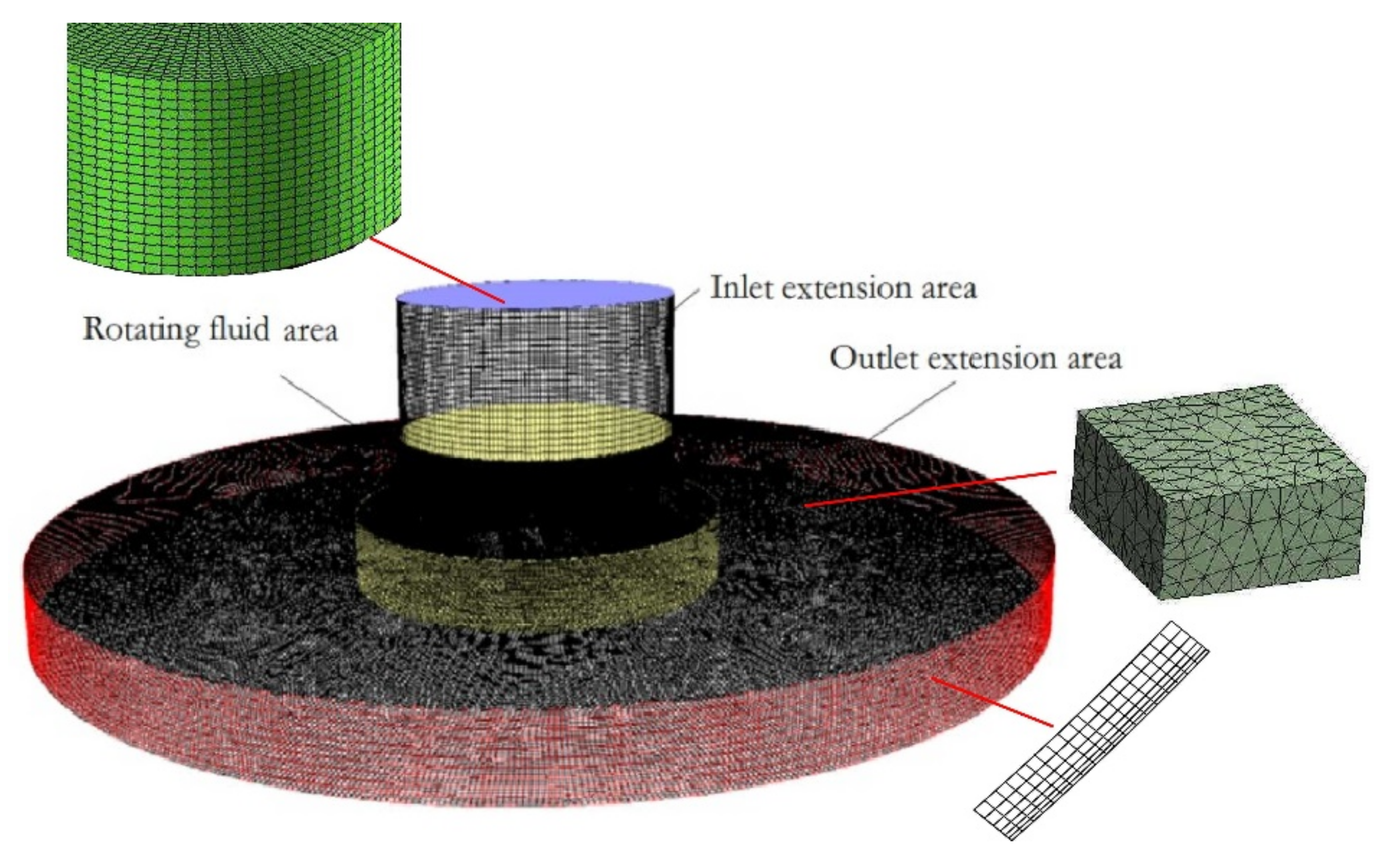
The finite volume analysis software Ansys Fluent [18] is used to simulate the centrifugal fan, and the flow field model of the fan is shown in Figure 5. The flow field model of fan is divided into three parts, which include inlet extension area, rotating fluid area, and outlet extension area. Besides, a multi-reference frame (MRF) approach is adopted for the rotating fluid area. The medium flowing in the fan channel is air, and the fluid in the fan moving area belongs to turbulence flow. The effect of gravity on the flow field is ignored. The standard k-ε model is used. In the simulation process, only the ambient pressure and its corresponding air physical properties are changed, while other boundary conditions are not changed. Given the complexity of the fan simulation model, a mixture of structured and unstructured grids is used to partition the fluid region. In the inlet extension and outlet extension areas, structured grid is adopted [19].

In the rotating fluid areas, the tetrahedral grid is used. The near-wall grids are locally encrypted. To assess the influence of the number of grids on the accuracy of the calculation, the grid independence is calculated. Five grid systems, 0.44 million, 0.72 million, 1 million,1.28 million, and 1.56 million, are tested. It is found that the relative errors of total pressure of fan between the solutions of 1.28 million and 1.56 million are less than 0.07%. It can be considered that the simulation calculation result is independent of the number of grids when the number of grids is encrypted to 1.28 million [20]. The inlet is set as “Velocity inlet”, the outlet is set as free “Outflow”, and the rotating fluid area is set as “no-slip boundary condition”.

4.2. Governing Equations

The governing equations mainly include mass conservation, momentum conservation, and energy conservation equations, which are

• Mass conservation equation

$$\frac{\partial \rho }{\partial \tau }+\nabla \cdot \left(\rho U\right)=0,$$

(6)

where U is the velocity vector, ρ is the density, and τ is time.

2.

Momentum conservation equation

$$\left.\begin{array}{l}\frac{\partial \left(\rho u_1\right)}{\partial \tau }+div(\rho u_1\cdot U)=div(\mu grad{u}_1)-\frac{\partial p}{\partial x}+S_u\\ \frac{\partial \left(\rho u_2\right)}{\partial \tau }+div(\rho u_2\cdot U)=div(\mu grad{u}_2)-\frac{\partial p}{\partial y}+S_v\\ \frac{\partial \left(\rho u_3\right)}{\partial \tau }+div(\rho u_3\cdot U)=div(\mu grad{u}_3)-\frac{\partial p}{\partial z}+S_w\end{array}\right\},$$

(7)

where μ is kinetic viscosity, p is pressure, u₁, u₂, and u₃ are the components of the velocity vector in the X, Y, and Z directions, and S_u, S_v, S_w are the generalized source terms.

3.

Energy conservation equation

$$\frac{\partial \left(\rho t\right)}{\partial t}+div\left(\rho Ut\right)=div(\frac{\lambda }{c_p}gradT)-\frac{\partial p}{\partial x}+S_T,$$

(8)

where T is the temperature, λ is the heat transfer coefficient of the fluid, c_p is the specific heat capacity, and S_T is the viscous dissipation term.

The solver uses the SEGREGATED separate implicit solver. The turbulence energy, turbulence dissipation term, and momentum conservation equations are all discretized using the second-order upwind scheme. The governing equations are solved using the transient-SIMPLE method. Second order upwind scheme is chosen to discretize these governing equations. Due to the strong nonlinear relationship between the variables, the iterative solution uses subrelaxation factors. The inlet and outlet turbulence are all set to 0.5%, and the detection surface of mass flow rate is set at the fan outlet section. For the mass conservation equation, when the results of two adjacent calculations are less than 10⁻⁶, the numerical simulation results can be considered to converge.

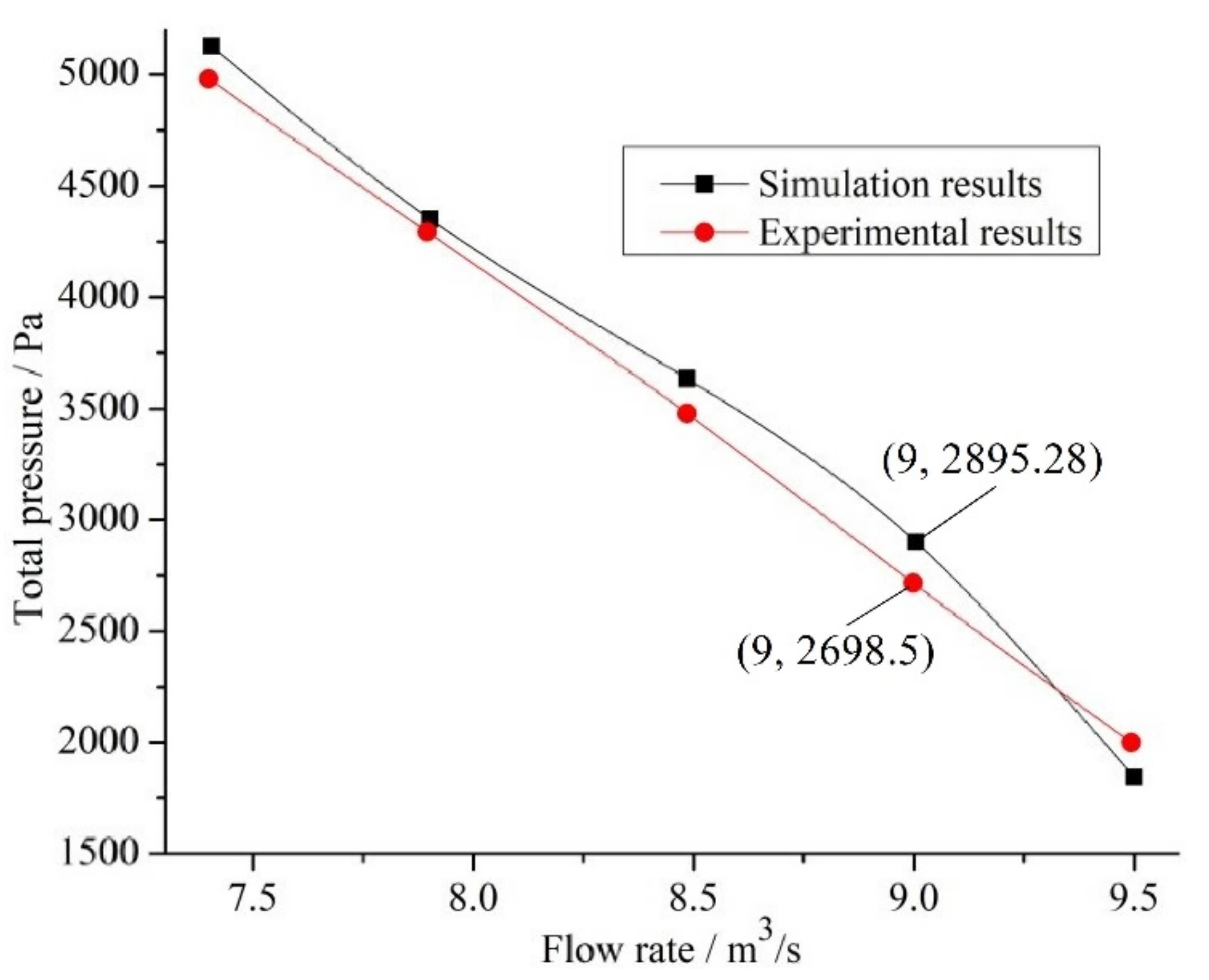
4.3. Simulation Model Verification

The diagram of the comparison between the simulation calculation results and the experimental results at the rotational speed of 5500 r/min under normal pressure is shown in Figure 6.

It can be seen from the figure that the error between the experimental value and the calculated value is within 6.8% in the whole experiment process, which indicates that the simulation model is reliable. The deviation between the simulation and the experimental results may be caused to some extent by the simplification of the fan model, measurement errors in the experimental process, and errors inherent in the simulation calculation method. At the same time, the simulation model is mainly used for comparative study. Therefore, the simulation model can be used to simulate the fan performance under different environmental pressures.

4.4. Numerical Calculation Results and Analysis

4.4.1. Pressure Analysis of the Fan under Different Ambient Pressures

Using this model, the performance of the fan under the same rotational speed (5500 r/min) and different ambient pressure is simulated, and the calculation results are shown in Figure 7.

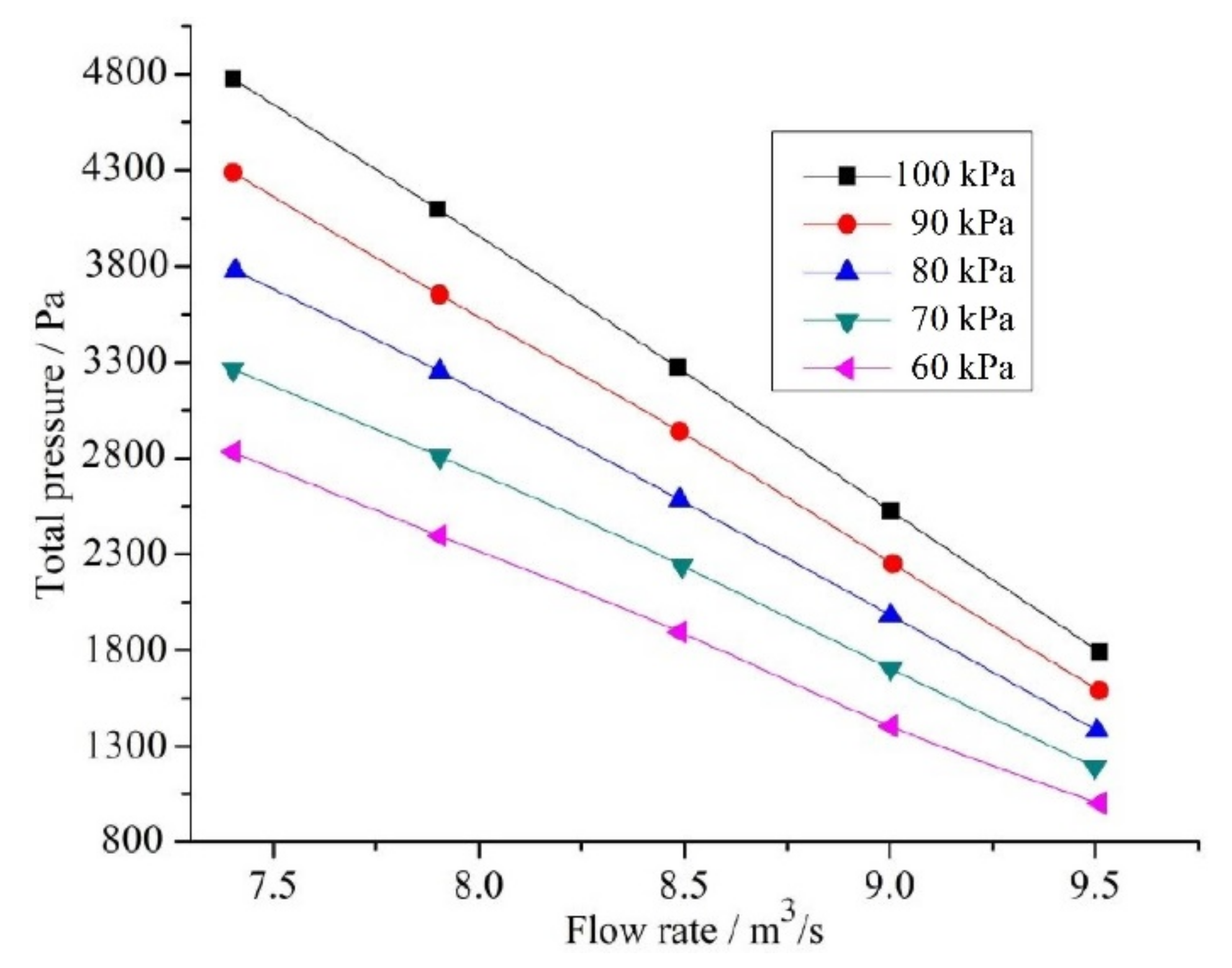
It can be seen from Figure 7 that the total pressure of the fan decreases with the decrease of flow rate, and the lower ambient pressure indicates that the total pressure of the fan is lower under the same condition. The quantitative analysis shows that compared with the normal pressure condition, the total pressure drop amplitude of the fan is basically the same at each working point under low pressure condition. Taking 60 kPa pressure operating point as an example, the average decrease range of total pressure of the fan is 42.3% compared with the normal pressure condition.

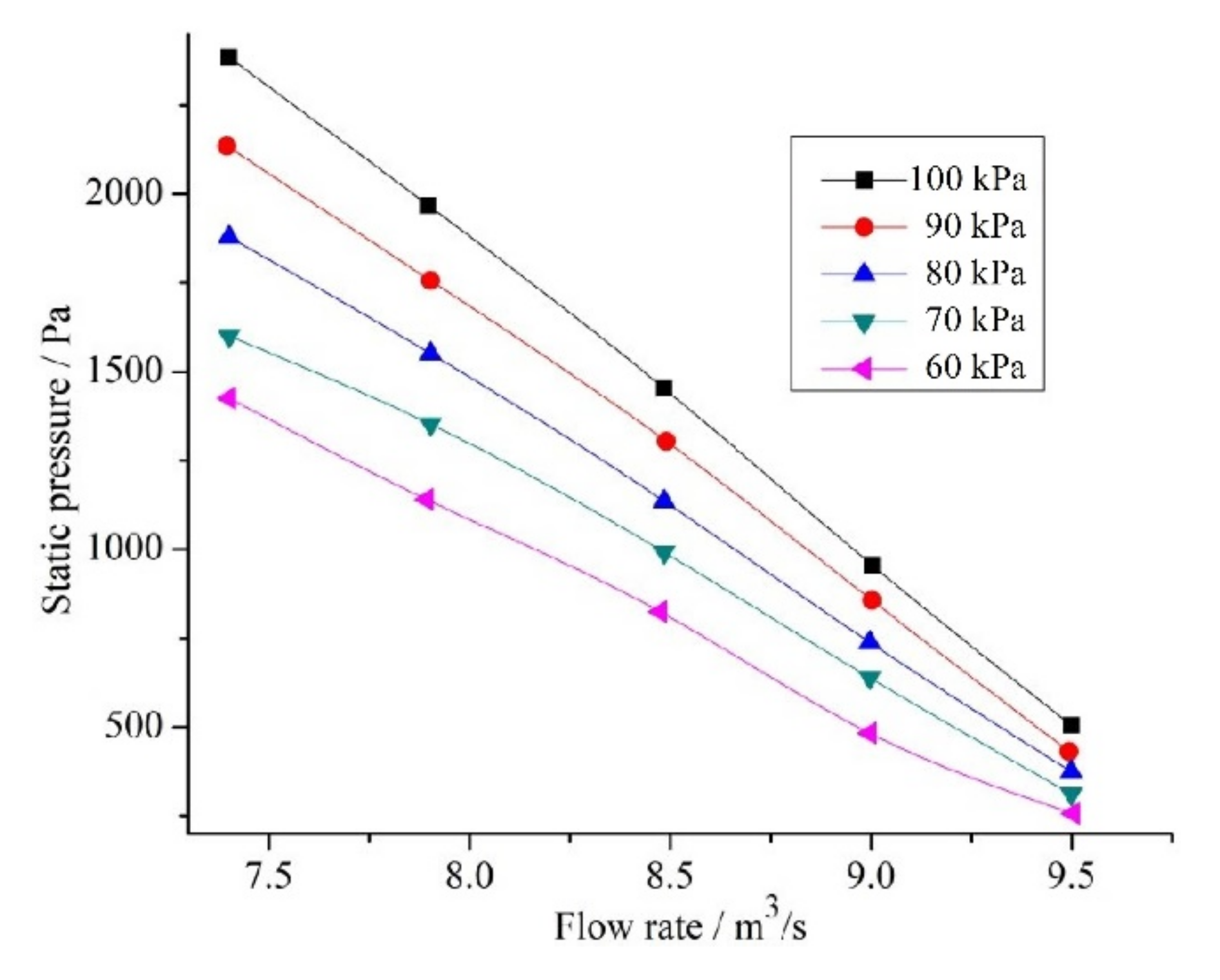
Figure 8 shows the changing curve of the static pressure versus flow rate of the fan under different ambient pressures. It can be seen from the figure that the variation trend of the fan static pressure and the total pressure is similar. The lower the ambient pressure, the lower the fan static pressure. Compared with the normal pressure condition, the static pressure drop extent of the fan is basically the same at each working point under the low-pressure condition. Taking 60 kPa pressure operating point as an example, the average decrease extent of fan static pressure is 38.3% compared with normal pressure operating point. At the same time, the air density at 60 kPa is about 39.5% lower than that at atmospheric pressure. Thus, the decline in the total pressure and static pressure performance of the fan is mainly due to the drop in the air density caused by the reduction of the environmental pressure.

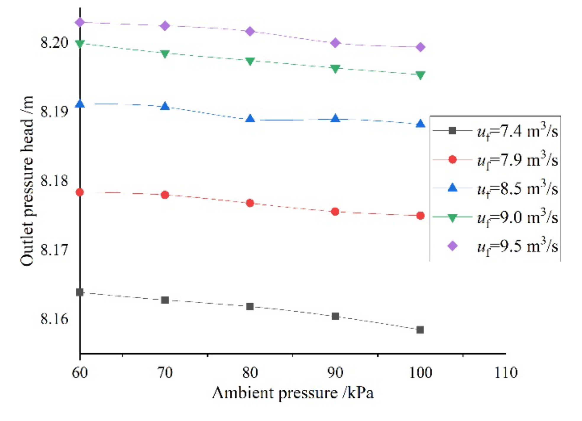
Figure 9 shows the change curve of fan outlet pressure head along with flow rate (u_f) under different ambient pressure. The figure shows that the outlet pressure head of the fan increases with the increase of flow rate (u_f) but changes little under different ambient pressure. It can be seen that the environmental pressure has little effect on the outlet pressure head of the fan. Although this change is not obvious, it can be found that the outlet pressure head decreases gradually with the increase of ambient pressure.

4.4.2. Noise Analysis under Different Ambient Pressure

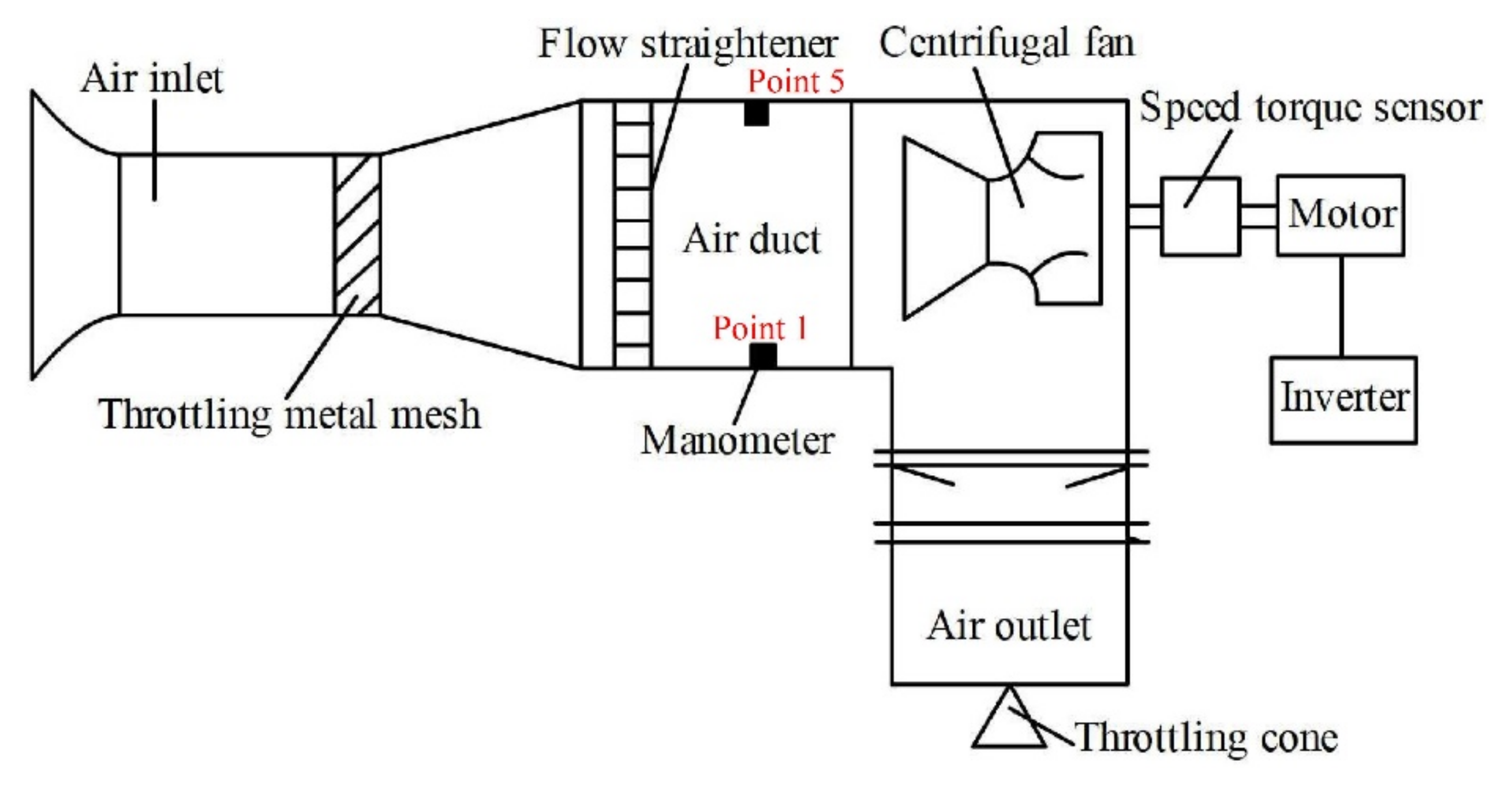
Fan noise propagation is an unsteady process. Large Eddy Simulation (LES) model is used to simulate the sound field, in which the time step is 0.01 ms and each time step is iterated 20 times. At the same time, two noise monitoring points (as shown in Figure 10) are set along the fan radial direction and axis central direction respectively for real-time monitoring of the sound pressure change of the fan. 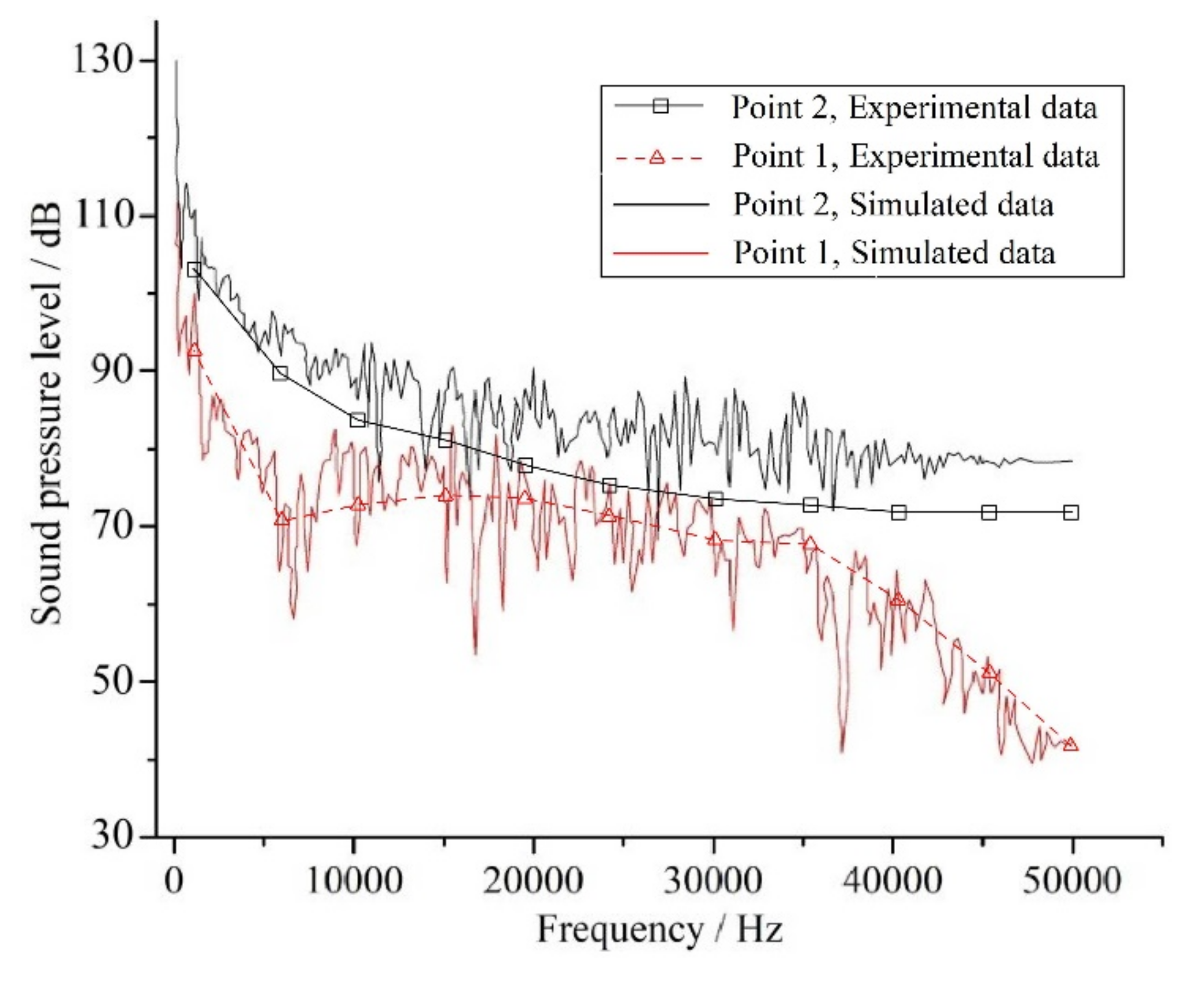The location of Point 1 and Point 2 are shown in Figure 10, and all dimensions are in millimetres [21,22]. The noise spectrogram of the prototype fan is shown in Figure 11 when the rotational speed of the fan is 5500 r/min and the flow rate is 8.5 m³/s at atmospheric pressure. It can also be seen from Figure 11 that although Point 1 is more than twice as far away from Point 2, the sound pressure level differs little at different frequencies. At the same time, for Point 2 in the axial direction, with the continuous increase of frequency (0–50,000 Hz), the sound pressure level gradually decreases and the trend eases. In the radial direction, with the increase of frequency, the variation of sound pressure level fluctuates greatly, which is the smallest when the frequency reaches 5000 Hz. This is because the change in axial pressure is much smaller than the change in radial pressure.

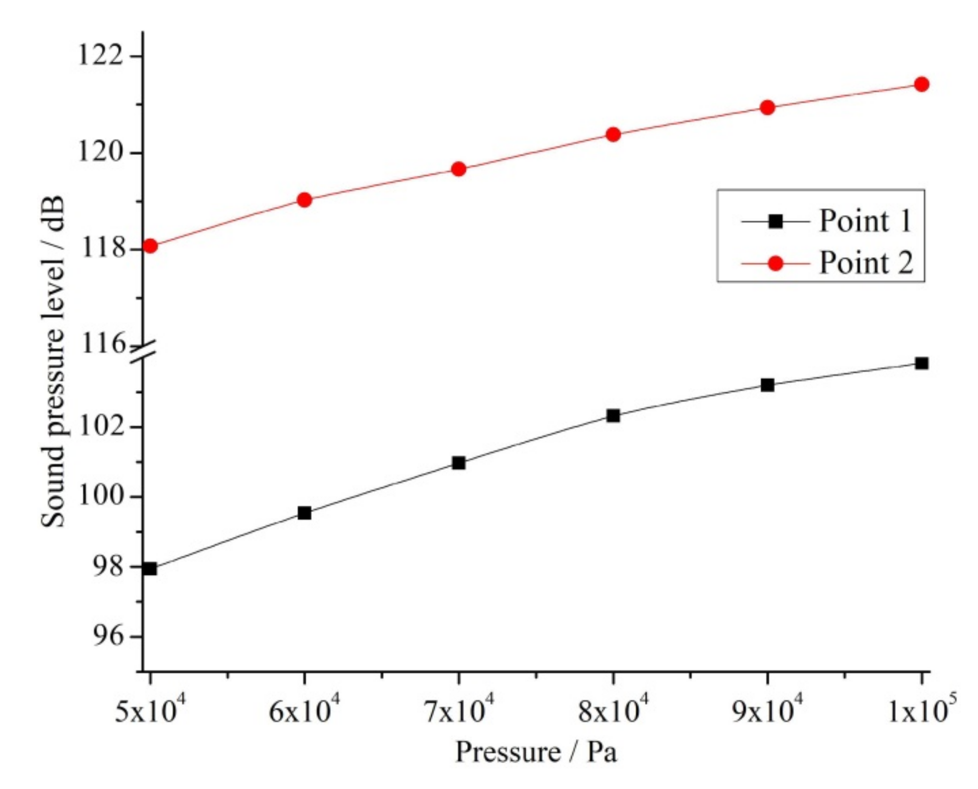
Changing the ambient pressure and fluid physical properties, the total sound pressure level of the prototype fan under different ambient pressures is obtained as shown in Figure 12. It can be seen from Figure 12 that as the ambient pressure decreases from 100 kPa to 50 kPa, the noise of the fan gradually becomes lower. In measurement Point 1, noise decreases from 103.85 dB to 98.2 dB. In measurement Point 2, it decreases from 121.45 dB to 118.1 dB. So, the sound pressure levels at the two measurement points decrease by about 5.8% and 2.8%, respectively. This means that the sound pressure level at negative pressure is smaller than that at one atmosphere. This also means that the noise produced by the centrifugal fan is less than that produced by one standard atmospheric pressure under the low-pressure environment such as the plateau environment. The general reason mainly lies in that the air density decreases when the air pressure is low, and the pressure variation range in the air during the operation of the centrifugal fan is small.

At the same time, with the decrease of ambient pressure, the sound pressure level of fan noise presents an approximate logarithmic reduction trend. The relationship between sound pressure level and sound power can be transformed into

$$L_P=10\lg \frac{W}{W_0}-20\lg r-11,$$

(9)

where W₀ is the reference sound power, and it is generally taken as 10⁻² W. As can be seen from Equation (9), we can obtain that L_p ~ lgW. Since the sound power W and the air density ρ are in a linear relationship, namely W ~ ρ, so L_p ~ lgρ, it can be seen that the logarithmic relationship of the sound pressure level and the air density is linear.

5. Conclusions

In this paper, the flow and noise characteristics of centrifugal fan in low-pressure environment (50 kPa–100 kPa) are studied; the following conclusions can be obtained:

• The sound power and sound pressure of the fan are proportional to the air density, while the sound pressure level of the fan is proportional to the logarithm of the air density.
• The total pressure and static pressure of the fan decrease with the decrease of environmental pressure. The total pressure and static pressure of the fan at 60 kPa pressure operating mode decrease by 42.3% and 38.3%, respectively, compared with the normal pressure. The main reason for this phenomenon is the decrease of air density due to the decrease of environmental pressure.
• Under the same working condition (fan rotational speed of 5500 r/min, flow rate of 8.5 m³/s), the sound pressure level at the two measuring points of the centrifugal fan increases by about 5.8% and 2.8%, respectively, as the ambient pressure increases from 50 kPa to 100 kPa. With the increase of ambient pressure, the sound pressure level of fan noise shows an approximate logarithmic growth trend.