Solution Polymerization of Acrylic Acid Initiated by Redox Couple Na-PS/Na-MBS: Kinetic Model and Transition to Continuous Process

Abstract

This work aims at modeling in detail the polymerization of non-ionized acrylic acid in aqueous solution. The population balances required to evaluate the main average properties of molecular weight were solved by the method of moments. The polymerization process considered is initiated by a persulfate/metabisulfate redox couple and, in particular, the kinetic scheme considers the possible formation of mid-chain radicals and transfer reactions. The proposed model is validated using experimental data collected in a laboratory-scale discontinuous reactor. The developed kinetic model is then used to intensify the discontinuous process by shifting it to a continuous one based on a tubular reactor with intermediate feeds. One of the experimental runs is selected to show how the proposed model can be used to assess the transition from batch to continuous process and allow faster scale-up to industrial scale using a literature approach.

1. Introduction

Poly(acrylic acid) (PAA) is a widely produced polymer with a growing, global annual production of $1.58\times {10}^9$ $\mathrm{k}\mathrm{g}$ as of 2008 [1] and with applications in many industrial sectors. The application is determined according to the molecular weight of the produced polymer: low molecular mass (less than 20 $\mathrm{k}$$\mathrm{Da}$) PAA is used as sequestrant, mid-low mass (20–80 $\mathrm{k}$$\mathrm{Da}$) PAA is adopted in paints, mid-high mass (0.1–1 $\mathrm{M}$$\mathrm{Da}$) PAA is useful in the textile and paper industry, and high weight (larger than 1 $\mathrm{M}$$\mathrm{Da}$) PAA is a flocculating agent and absorbent [1]. The accurate control of the average molecular weight and its distribution are thus critical for efficient production.

The synthesis of PAA is almost exclusively run in aqueous solutions through free-radical polymerization of acrylic-acid (AA) at 40–90 ${}^{\circ }\mathrm{C}$ in batch (BR) or semi-batch (SBR) chemical reactors. The reaction is highly exothermic (reaction heat of 63 $\mathrm{k}$$\mathrm{J}$ ${\mathrm{mol}}^{-1}$ [2]) and fast, posing a relevant hazard for its production in discontinuous BR systems. The SBR is then preferred as a more efficient thermal control can be achieved with respect to its BR counterpart. A SBR starved process is generally adopted to achieve such control in a monomer-depleted environment. This way AA is consumed at a faster rate than its dosing and no dangerous accumulation of monomer is taking place. On the other hand, this kind of process may require long reaction times and proper disposal of the high amount of water used.

A way to enhance the performance of the PAA production is to shift the discontinuous process to a continuous one by means, for example, of tubular reactors in the general framework of process intensification [3]. Tubular reactors are more efficient in the thermal control with respect to both BRs and SBRs [4] thanks to the higher heat-exchange-area-to-volume ratio. This way, more severe conditions can be used with reduction of both reaction times and downstream utilities. Several methods were developed to shift polymerization processes from batch to continuous, by means of modular reactors (given a particular process) [5,6] or tubular reactors with distributed and localized side injections (for any homogeneous system regardless the chemical kinetics) [7,8].

Typically, the process conditions are designed according to the selected initiating system and the desired product quality (its molecular weight distribution). Commonly used initiators are azo compunds, e.g., azobis-isobutyronitrile (AIBN) and 2,2′-azobis-(2-methyl propionamidine) dihydrochloride (V-50), peroxides, e.g., benzoyl peroxide, and redox initiators, such as persulfate/metabisulfate (PS/MBS) couples [9]. A detailed description of the chemical transformations happening in the reactor is thus paramount to develop processes (both discontinuous and continuous) able to produce the desired product in the most efficient way. A large body of work was carried out (in discontinuous reactors) to accurately determine the reaction rates of AA polymerization. Much effort was spent towards the description of propagation reactions, taking into account many effects such as the initial presence of monomer in the reaction environment [10,11], pH, and the degree of AA dissociation [12,13]. AA radicals also undergo backbiting, leading to the formation of mid-chain radicals (MCR) from which branching occurs [14]. According to the initiating system used, other reactions can occur such as radical transfer to the co-initiator in a redox system [15].

The aim of this work is the development of a comprehensive chemical reaction model for the polymerization of fully-undissociated AA in aqueous solution using the couple PS/MBS as redox initiator. The model is validated with experimental measurements on the discontinuous system. The developed model is then used for process intensification, with emphasis on the transition from discontinuous to continuous production processes.

2. Materials and Methods

2.1. Experimental Tests

2.1.1. Chemicals and Analytical Technique

The experimental tests were run using acrylic acid (99%), sodium persulfate (Na-PS, ≥$98\%$), sodium metabisulfate (Na-MBS, ≥$99\%$), hydroquinone (≥$99\%$), sodium nitrate (≥$99\%$), monobasic sodium phosphate monohydrate (≥$98\%$), and sodium azide (≥$99\%$). All chemicals were purchased from Sigma-Aldrich and were used as received without further purification.

For each reaction condition several samples were taken over time. The reaction was inhibited by adding the sample to cold hydroquinone. The samples were then analyzed using gel permeation chromatography (GPC) for the determination of the polymer molecular weight distributions. GPC measurements were carried out at 30 ${}^{\circ }\mathrm{C}$ using a pH 7 buffer mixture of aqueous solutions of sodium nitrate ($0.2$ M), monobasic sodium phosphate ($0.01$ M), and sodium azide ($3.1$ $\mathrm{m}$M) as eluent with a flowrate of 1 $\mathrm{m}$$\mathrm{L}$ ${\min }^{-1}$. The calibration of the instrument was made using PAA standards with certified peak molecular weights from 1250 to 392,600 $\mathrm{g}$ ${\mathrm{mol}}^{-1}$ (all details as Supplementary Materials), thus enabling especially accurate molecular weight evaluations in the range of interest.

Residual monomer was detected by high-performance liquid chromatography (HPLC) equipped with UV detector (wavelength 205 $\mathrm{n}$$\mathrm{m}$) and a column suitable for organic acids. In all cases, the eluent was an aqueous solution of sulfuric acid $0.05$ M and the flowrate $0.5$ $\mathrm{m}$$\mathrm{L}$ ${\min }^{-1}$.

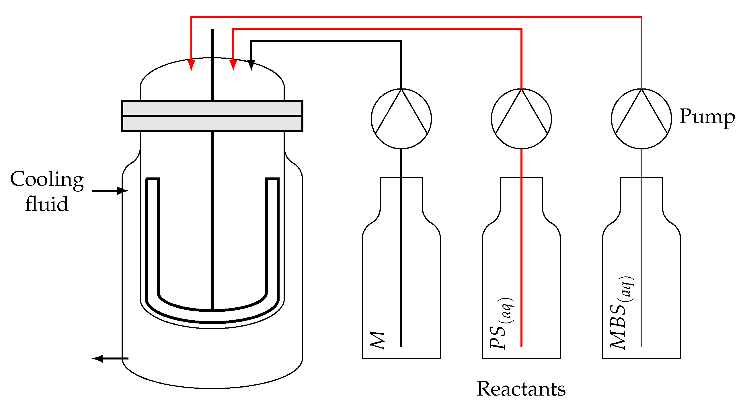
2.1.2. Discontinuous Reactor

The laboratory SBR is a jacketed glass reactor with a maximum volume of 1 $\mathrm{L}$, equipped with mechanical stirring and reflux condenser. The reagents were fed using three Metrohm 876 Dosimat plus dosing units. PS and MBS are fed into the reactor as aqueous solutions, while the monomer is fed as a pure stream. A schematic representation of the experimental setup is reported in Figure 1.

Species are fed into the reactor with a constant feedrate and different feed durations. In particular, PS and MBS are fed together from the beginning of the process into the reactor, which was initially charged with pure water. After a constant delay, $\Delta t_M^0$, the monomer feed is started. Once the entire mass of monomer, $m_M^F$, is fed over up to the dosing time $t_M^F$, the PS and MBS aqueous solutions are fed for some more time, $\Delta t_{PS}^F$ and $\Delta t_{MBS}^F$ respectively. The total quantities of salts fed into the reactor are $m_{PS}^F$ and $m_{MBS}^F$ for PS and MBS, respectively. Water is also fed into the reactor, as the salts are diluted in aqueous solution; the quantity of water used to dilute the salts is equal to $m_{W,PS}^F$ and $m_{W,MBS}^F$ for PS and MBS, respectively. All species were fed into the reactor at a constant rate. The experimental values of the aforementioned quantities can be found in

Table 1. Settings of the SBR tests and available number of specimen over time for each set.

Test	${\mathit{m}}_{\mathit{M}}^{\mathit{F}}$	${\mathit{m}}_{\mathit{PS}}^{\mathit{F}}$	${\mathit{m}}_{\mathit{MBS}}^{\mathit{F}}$	${\mathit{m}}_{\mathit{W},\mathit{PS}}^{\mathit{F}}$	${\mathit{m}}_{\mathit{W},\mathit{MBS}}^{\mathit{F}}$	${\mathit{m}}_{\mathit{W}}^0$	T	${\mathit{t}}_{\mathit{M}}^{\mathit{F}}$	N${}^{\circ }$ Data
	[g]	[g]	[g]	[g]	[g]	[g]	[${}^{\circ }$C]	[h]
SBR1	280	7.8	44.44	37.8	66.66	137.8	90	5	6
SBR2	280	7.8	44.44	37.8	66.66	137.8	90	0.5	4
SBR3	252	7.0	40.00	34.0	60.00	124.0	75	5	6
SBR4	280	7.8	22.24	37.8	33.36	137.8	70	5	6
SBR5	280	7.8	44.44	37.8	66.66	137.8	50	5	6
SBR6	280	7.8	22.24	37.8	33.36	137.8	90	5	6
SBR7	28	0.78	4.444	3.78	6.666	231.8	90	5	6
SBR8	315	8.8	50.00	42.5	75.00	155.0	90	2.5	6
SBR9	252	7.0	40.00	34.0	60.00	124.0	90	1.5	6
SBR10	280	7.8	44.44	37.8	66.66	137.8	90	5	6
SBR11	280	7.8	44.44	37.8	66.66	137.8	90	2.5	6
SBR12	280	7.8	44.44	37.8	66.66	137.8	90	1	6
SBR13	280	7.8	11.12	37.8	16.68	137.8	90	5	6
SBR14	28	0.78	0.00	3.78	0.00	231.8	90	5	6
SBR15	280	7.8	0.00	37.8	0.00	275.6	70	5	4
SBR16	280	7.8	11.12	37.8	16.68	137.8	70	5	6
SBR17	280	7.8	11.12	37.8	16.68	137.8	60	5	6

with the exception of the $\Delta t$ mentioned above. Such values cannot be disclosed because they are proprietary data.

3. Model Development

3.1. Kinetic Scheme

The considered kinetic scheme extends the basic structure of a polymerization process (initiation, propagation, and termination by both combination and disproportionantion) by adding the possibility of backbiting (formation of MCRs; such radicals are identified by the superscript s while regular terminal radicals by the superscript t) and transfer reactions. The monomer is assumed to be non-ionized, as the $p{K}_a$ of AA is equal to 4.25 at ambient temperature [16], thus corresponding to a degree of ionization lower than 1%. All reactions are treated as irreversible, elementary reactions, thus their reaction rate is given by a rate constant multiplied by the product of the molar concentrations (indicated in square brackets in the following) of the reactants involved.

The initiation step is due to a redox reaction between PS and MBS [17,18] as well as to the thermal decomposition reaction of PS [19], both reactions producing two radicals:

$$\underset{PS}{\underbrace{S_2{O}_8^{2-}}}+\underset{MBS}{\underbrace{S_2{O}_3^{2-}}}\to \underset{2R_0}{\underbrace{S{O}_4^{•-}+{}^{•}{S}_2{O}_3^{-}}}+S{O}_4^{2-}$$

(1)

$$PS\to \underset{2R_0}{\underbrace{2S{O}_4^{•-}}}$$

(2)

No distinction was done between the radicals formed in the initiation step, by assuming they have the same reactivity towards all other species, and they will be simply indicated as $R_0$.

Na-MBS is a known chain-transfer agent [15], thus the kinetic scheme also considers the transfer reactions to monomer and MBS. This is a particular reaction arising from the use of MBS and is generally not present in classical kinetic schemes. Transfer to the monomer can also occur [14], while the transfer reaction to dead chains (polymers) was observed to be negligible under the investigated conditions and it is generally not accounted for [14]. Transfer to water was considered negligible, compared to other transfer mechanisms [10].

Termination reactions can occur between any kind of radical, both of the same type (ss, tt) or of different types (st). The distinction between termination by combination or by disproportionation is quantified with a proper constant $\kappa$ according to the type of radicals involved in the termination reaction.

The complete set of chemical reactions is reported in

Table 2. Chemical reaction mechanism and reaction rates for the dissociated AA polymerization in water initiated by PS/MBS redox couple.

Name	Reaction	Rate
Initiation	$PS+MBS\to 2R_0+S{O}_4^{2-}$	$k_1\left[PS\right]\left[MBS\right]$
	$PS\to 2R_0$	$k_d\left[PS\right]$, efficiency f
Propagation	$R_n^s+M\to R_{n+1}^s$	$k_p^s\left[M\right]\left[R_n^s\right]$
	$R_n^t+M\to R_{n+1}^s$	$k_p^t\left[M\right]\left[R_n^t\right]$
Backbiting	$R_n^s\to R_n^t$	$k_{bb}\left[R_n^s\right]$
Transfer to monomer	$R_n^s+M\to P_n+R_1^s$	$k_{trM}^s\left[M\right]\left[R_n^s\right]$
	$R_n^t+M\to P_n+R_1^s$	$k_{trM}^t\left[M\right]\left[R_n^t\right]$
Transfer to MBS	$R_n^s+MBS\to P_n+R_0$	$k_{trMBS}^s\left[MBS\right]\left[R_n^s\right]$
	$R_n^t+MBS\to P_n+R_0$	$k_{trMBS}^t\left[MBS\right]\left[R_n^t\right]$
Termination by	$R_n^s+R_m^s\to P_{n+m}$	$k_t^{ss}(1-{\kappa }^{ss})\left[R_n^s\right]\left[R_m^s\right]$
combination	$R_n^s+R_m^t\to P_{n+m}$	$k_t^{st}(1-{\kappa }^{st})\left[R_n^s\right]\left[R_m^t\right]$
	$R_n^t+R_m^t\to P_{n+m}$	$k_t^{tt}(1-{\kappa }^{tt})\left[R_n^t\right]\left[R_m^t\right]$
Termination by	$R_n^s+R_m^s\to P_n+P_m$	$k_t^{ss}{\kappa }^{ss}\left[R_n^s\right]\left[R_m^s\right]$
disproportionation	$R_n^s+R_m^t\to P_n+P_m$	$k_t^{st}{\kappa }^{st}\left[R_n^s\right]\left[R_m^t\right]$
	$R_n^t+R_m^t\to P_n+P_m$	$k_t^{tt}{\kappa }^{tt}\left[R_n^t\right]\left[R_m^t\right]$

along with each reaction rate computed from the molar concentration of species (reported in square brackets). The monomer is indicated as M, terminal radicals of length n as $R_n^s$, MCRs of length n as $R_n^t$, while polymers of length n as $P_n$ (regardless their branching structure). It is assumed terminal radicals and MCR have different reactivity as reported in Table 2.

3.2. Governing Equations

It is assumed that all reactors are isothermal, then characterized by constant and uniform temperature value. Mixing is assumed to be perfect in the SBR while plug-flow behavior is assumed in the tubular reactor. AA monomer will be indicated as M, water as W, Na-PS as $PS$, Na-MBS as $MBS$, and polymer (PAA) as P.

The model for the SBR is initially developed and applied to validate the proposed kinetic scheme using experimental data. Then, the model for the continuous system is presented, with reference to tubular reactors. Finally, a kinetics-free procedure, which details can be found elsewhere [7,8], is applied to adapt the recipe already effective in SBR to a continuous production process based on a series of tubular reactors with intermediate feed streams.

3.2.1. SBR Model

For every species i it is possible to write a molar conservation equation:

$$\frac{d{n}_i}{dt}=F_i+R_{i}V$$

(3)

for $i=1\cdots NC$, where $NC$ is the number of components (species), $n_i$ the number of moles of species i in the SBR at a given time, t, $F_i$ the (possibly-non-constant) molar feed-rate of species i at a given time, $R_i$ the production rate of species i as a function of temperature, T, and composition, and V the reaction volume at a given time. This equation is equipped with the initial condition:

$$n_i\left(0\right)=\frac{m_i^0}{M{W}_i}$$

(4)

where $m_i^0$ is the mass of species i which is initially charged into the reactor and $M{W}_i$ is species i molecular weight. For the test run in this work, only water is initially charged into the reactor, thus $m_i^0=0$ for all species except water.

The molar flowrate changes in time according to:

$$F_M=\frac{m_M^F}{M{W}_M(t_M^F-\Delta t_M^0)}H(t-\Delta t_M^0)H(t_M^F-t)$$

(5)

$$F_{PS}=\frac{m_{PS}^F}{M{W}_{PS}(t_M^F+\Delta t_{PS}^F)}H(t_M^F+\Delta t_{PS}^F-t)$$

(6)

$$F_{MBS}=\frac{m_{MBS}^F}{M{W}_{MBS}(t_M^F+\Delta t_{MBS}^F)}H(t_M^F+\Delta t_{MBS}^F-t)$$

(7)

$$F_W=\frac{m_{W,PS}^F}{M{W}_W(t_M^F+\Delta t_{PS}^F)}H(t_M^F+\Delta t_{PS}^F-t)+\frac{m_{W,MBS}^F}{M{W}_W(t_M^F+\Delta t_{MBS}^F)}H(t_M^F+\Delta t_{MBS}^F-t)$$

(8)

where $H\left(t\right)$ the Heaviside function. These functions take into account all the delays happening in the experimental runs. All other species (namely, radicals and polymers) have a null feedrate. The species production rate is given by:

$$R_i=\sum _n^{NR}{\nu }_{in}{r}_n$$

(9)

where $NR$ is the number of reactions happening in the system, ${\nu }_{in}$ the stoichiometric coefficient of species i in reaction n, and $r_n$ the n-th reaction rate, as from Table 2.

Under the assumption of ideal mixtures, species volumes can be considered to be additive, meaning:

$$V=\sum _i^{NC}\frac{m_i}{{\rho }_i}\approx \frac{m_W+m_{PS}+m_{MBS}}{{\rho }_W}+\frac{m_M}{{\rho }_M}+\frac{m_P}{{\rho }_P}$$

(10)

where $m_i=n_{i}M{W}_i$ is the mass of species i at a given time, and ${\rho }_i$ the density of pure species i at a given temperature. The pure species density is provided in

Table 3. Pure species density as a function of temperature [14,20]. Temperature in [${}^{\circ }\mathrm{C}$].

Species	Density [g cm${}^{-3}$]
W	$0.9999+2.3109\times {10}^{-5}T-\mathrm{5.448,07}\times {10}^{-6}{T}^2$
M	$1.0731-1.0826\times {10}^{-3}T-7.2379\times {10}^{-7}{T}^2$
P	$1.7-6.0\times {10}^{-4}T$

as a polynomial function of temperature.

To solve the polymer population balances in an effective way, the method of moments (MoM) is used. By definition, the moments of a generic order k are:

$${\lambda }_k^s=\sum _{j=1}^{\infty }{j}^k{n}_{R_j^s}$$

(11)

$${\lambda }_k^t=\sum _{j=1}^{\infty }{j}^k{n}_{R_j^t}$$

(12)

$${\mu }_k=\sum _{j=1}^{\infty }{j}^k{n}_{P_j}$$

(13)

respectively, the k-th order moment of the secondary radicals, tertiary radicals, and dead polymers. $n_{R_j^s}$ is the number of moles of the secondary radicals of length j, $n_{R_j^t}$ for tertiary radicals, and $n_{P_j}$ for dead chains. The moments behave as pseudo-species, representing the ensemble of radicals and polymers, thus they change in time as reaction proceeds.

This way the main average properties of the molecular weight distribution can be easily computed. In particular, the number-average chain length (number-average degree of polymerization) is:

$$D{P}_n=\frac{{\sum }_{j=1}^{\infty }j{n}_{P_j}}{{\sum }_{j=1}^{\infty }{n}_{P_j}}=\frac{{\mu }_1}{{\mu }_0}$$

(14)

the weight-average chain length (weight-average degree of polymerization) is:

$$D{P}_w=\frac{{\sum }_{j=1}^{\infty }{j}^2{n}_{P_j}}{{\sum }_{j=1}^{\infty }j{n}_{P_j}}=\frac{{\mu }_2}{{\mu }_1}$$

(15)

and the polydispersity is:

$$Đ=\frac{D{P}_w}{D{P}_n}=\frac{{\mu }_2{\mu }_0}{{\mu }_1^2}$$

(16)

Furthermore, the average radical chain length can be computed as:

$$D{P}_n^R=\frac{{\lambda }_1^s+{\lambda }_1^t}{{\lambda }_0^s+{\lambda }_0^t}$$

(17)

The minimum number of moments to be computed is therefore three for the polymer (${\mu }_0$, ${\mu }_1$, ${\mu }_2$) and two for each type of radicals (${\lambda }_0^s$, ${\lambda }_0^t$, ${\lambda }_1^s$, ${\lambda }_1^t$). If of interest, additional moments could be used to get more detailed information on the molecular weight distribution.

Using the definitions of moments, it is possible to write equations describing their change in time, exploiting the fact that for radicals and polymers no convective term is present (the feedrate is null). From Equation (3):

$$\frac{d{\lambda }_k^s}{dt}=\sum _{j=1}^{\infty }{j}^k\frac{d{n}_{R_j^s}}{dt}=\sum _{j=1}^{\infty }{j}^k{R}_{R_j^s}V=R_{{\lambda }_k^s}V$$

(18)

$$\frac{d{\lambda }_k^t}{dt}=\sum _{j=1}^{\infty }{j}^k\frac{d{n}_{R_j^t}}{dt}=\sum _{j=1}^{\infty }{j}^k{R}_{R_j^t}V=R_{{\lambda }_k^t}V$$

(19)

$$\frac{d{\mu }_k}{dt}=\sum _{j=1}^{\infty }{j}^k\frac{d{n}_{P_j}}{dt}=\sum _{j=1}^{\infty }{j}^k{R}_{P_j}V=R_{{\mu }_k}V$$

(20)

Furthermore, as no radical nor polymer is present at the beginning of the reaction, the initial quantity of all moments is null, meaning ${\lambda }_k^s\left(0\right)={\lambda }_k^t\left(0\right)={\mu }_k\left(0\right)=0$.

Using the reaction rates reported in Table 2, one can write the production rates of the molecular species, as well as those of the moments:

$$R_M=-k_p^s\left[M\right]\left[R_0\right]-(k_p^s+k_{trM}^s)\left[M\right]\left[{\lambda }_0^s\right]-(k_p^t+k_{trM}^t)\left[M\right]\left[{\lambda }_0^t\right]$$

(21)

$$R_W=0$$

(22)

$$R_{PS}=-k_1\left[PS\right]\left[MBS\right]-k_d\left[PS\right]$$

(23)

$$R_{MBS}=-k_1\left[PS\right]\left[MBS\right]-(k_{trMBS}^s\left[{\lambda }_0^s\right]+k_{trMBS}^t\left[{\lambda }_0^t\right])\left[MBS\right]$$

(24)

$$\begin{array}{cc}\hfill R_{{\lambda }_k^s}& =k_p^s\left[M\right]\left[R_0\right]+k_p^s\left[M\right]\sum _{l=0}^k\left(\genfrac{}{}{0pt}{}{k}{l}\right)\left[{\lambda }_l^s\right]-k_p^s\left[M\right]\left[{\lambda }_k^s\right]-k_{bb}\left[{\lambda }_k^s\right]+k_p^t\left[M\right]\sum _{l=0}^k\left(\genfrac{}{}{0pt}{}{k}{l}\right)\left[{\lambda }_l^t\right]+\hfill \\ \hfill & +k_{trM}^s\left[M\right](\left[{\lambda }_0^s\right]-\left[{\lambda }_k^s\right])+k_{trM}^t\left[M\right]\left[{\lambda }_0^t\right]-k_{trMBS}^s\left[{\lambda }_k^s\right]\left[MBS\right]-k_t^{ss}\left[{\lambda }_0^s\right]\left[{\lambda }_k^s\right]-k_t^{st}\left[{\lambda }_k^s\right]\left[{\lambda }_0^t\right]\hfill \end{array}$$

(25)

$$R_{{\lambda }_k^t}=k_{b}b\left[{\lambda }_k^s\right]-k_p^t\left[M\right]\left[{\lambda }_k^t\right]-k_{trMBS}^t\left[{\lambda }_k^t\right]\left[MBS\right]-k_t^{st}\left[{\lambda }_0^s\right]\left[{\lambda }_k^t\right]-k_t^{tt}\left[{\lambda }_0^t\right]\left[{\lambda }_k^t\right]$$

(26)

$$\begin{array}{cc}\hfill R_{{\mu }_k}& =k_{trM}^s\left[M\right]\left[{\lambda }_k^s\right]+k_{trM}^t\left[M\right]\left[{\lambda }_k^t\right]+\left(k_{trMBS}^s\left[{\lambda }_k^s\right]+k_{trMBS}^t\left[{\lambda }_k^t\right]\right)\left[MBS\right]+\hfill \\ \hfill & +\frac{1}{2}\left(k_t^{ss}(1-{\kappa }^{ss})\sum _{l=0}^k\left(\genfrac{}{}{0pt}{}{k}{l}\right)\left[{\lambda }_l^s\right]\left[{\lambda }_{k-l}^s\right]+k_t^{st}(1-{\kappa }^{st})\sum _{l=0}^k\left(\genfrac{}{}{0pt}{}{k}{l}\right)\left[{\lambda }_l^s\right]\left[{\lambda }_{k-l}^t\right]+\right.\hfill \\ \hfill & \left.+k_t^{tt}(1-{\kappa }^{tt})\sum _{l=0}^k\left(\genfrac{}{}{0pt}{}{k}{l}\right)\left[{\lambda }_l^t\right]\left[{\lambda }_{k-l}^t\right]\right)+k_t^{ss}{\kappa }^{ss}\left[{\lambda }_0^s\right]\left[{\lambda }_k^s\right]+k_t^{st}{\kappa }^{st}\left(\left[{\lambda }_k^s\right]\left[{\lambda }_0^t\right]+\left[{\lambda }_0^s\right]\left[{\lambda }_k^t\right]\right)+\hfill \\ \hfill & +k_t^{tt}{\kappa }^{tt}\left[{\lambda }_0^t\right]\left[{\lambda }_k^t\right]\hfill \end{array}$$

(27)

The molar concentration of species i is given by the ratio $n_i/V$, while the concentration of moments is given by the ratio between moment and volume.

Assuming quasi-steady-state conditions for the radicals produced during initiation, the consumption rate is approximated by the propagation rate only (being this term much higher than any other consumption term), meaning:

$$R_{R_0}\approx 2f{k}_d\left[PS\right]+2k_1\left[PS\right]\left[MBS\right]+(k_{trMBS}^s\left[{\lambda }_0^s\right]+k_{trMBS}^t\left[{\lambda }_0^t\right])\left[MBS\right]-k_p^S\left[M\right]\left[R_0\right]=0$$

(28)

from which it is possible to compute analytically the concentration of radicals (of length zero):

$$\left[R_0\right]=\frac{2f{k}_d\left[PS\right]+2k_1\left[PS\right]\left[MBS\right]+(k_{trMBS}^s\left[{\lambda }_0^s\right]+k_{trMBS}^t\left[{\lambda }_0^t\right])\left[MBS\right]}{k_p^S\left[M\right]}$$

(29)

The mass fraction of species i can be expressed as:

$${\omega }_i=\frac{m_i}{{\displaystyle \sum _i^{NC}\left(m_i^0+M{W}_i{\int }_0^t{F}_i\left(\tau \right)d\tau \right)}}$$

(30)

where $\tau$ is an auxiliary variable of integration. The initial mass fraction of monomer is ${\omega }_M^0=m_M^0/{\sum }_i^{NC}{m}_i^0$.

The monomer overall conversion at a given time is defined, for the SBR, as

$$\chi =\frac{{\displaystyle m_M^0+M{W}_M{\int }_0^t{F}_M\left(\tau \right)d\tau -M{W}_M{n}_M}}{m_M^0+m_M^F}$$

(31)

while the instantaneous conversion is

$$\mathcal{I}=1-\frac{M{W}_M{n}_M}{{\displaystyle m_M^0+M{W}_M{\int }_0^t{F}_M\left(\tau \right)d\tau }}$$

(32)

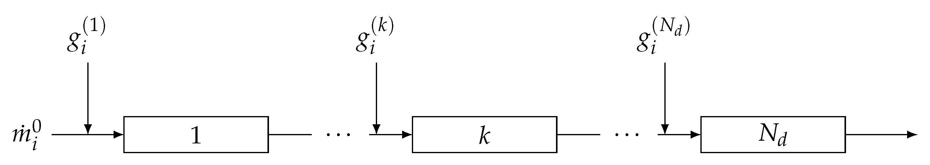
3.2.2. Tubular Reactor Model

In a similar manner, a tubular reactor model can be written under the assumption of uniform distribution of species over the cross section of the reactor. This condition can be fulfilled in different ways, e.g., by using static mixers. Accordingly the tubular reactor can be modeled as a plug-flow reactor (PFR) [21]. A series of PFRs with intermediate feedings (depicted in Figure 2) can be modeled by noting that the inlet stream to one reactor is equal to the outlet stream from the previous one with the addition of the intermediate stream. The model is therefore able to describe the single PFR and proper boundary conditions are used to link the PFRs in the series.

For each species i the molar conservation equation along the axial coordinate of the reactor, x, in terms of molar flowrates reads:

$$\frac{d{\dot{n}}_i}{dx}=R_i\mathcal{A}$$

(33)

where ${\dot{n}}_i$ is species i molar flowrate at a given axial position, and $\mathcal{A}$ is the cross-sectional area of the reactor (assumed uniform along the axial coordinate). $R_i$ is computed as from Equation (9). The boundary condition at the entrance of the reactor is:

$${\dot{n}}_i\left(0\right)=\frac{{\dot{m}}_i^{prev}+g_i}{M{W}_i}$$

(34)

where ${\dot{m}}_i^{prev}$ is the outlet mass flowrate of species i from the previous reactor and $g_i$ the intermediate feedrate of species i pertaining to the considered PFR of the series (note that $g_i$ can be non-uniform along the series of PFRs). For the first reactor in the series ${\dot{m}}_i^{prev}={\dot{m}}_i^0$ is the mass flowrate of species i fed at the entrance of the series of PFRs. The values of the inlet and intermediate feedrates, along with their composition, are computed through a kinetics free procedure according to the number of reactors in the series, $N_d$, starting from a given SBR recipe [7,8]. All reactors in the series are assumed to have the same geometrical parameters (length and cross-sectional area).

Under the assumption of ideal mixtures, the volumetric flowrate can be computed in a given position as:

$$\dot{V}=\sum _i^{NC}\frac{{\dot{m}}_i}{{\rho }_i}\approx \frac{{\dot{m}}_W+{\dot{m}}_{PS}+{\dot{m}}_{MBS}}{{\rho }_W}+\frac{{\dot{m}}_M}{{\rho }_M}+\frac{{\dot{m}}_P}{{\rho }_P}$$

(35)

where ${\dot{m}}_i={\dot{n}}_{i}M{W}_i$ is the mass flowrate of species i in the same position.

The MoM is again applied with the following definitions:

$${\lambda }_k^s=\sum _{j=1}^{\infty }{j}^k{\dot{n}}_{R_j^s}$$

(36)

$${\lambda }_k^t=\sum _{j=1}^{\infty }{j}^k{\dot{n}}_{R_j^t}$$

(37)

$${\mu }_k=\sum _{j=1}^{\infty }{j}^k{\dot{n}}_{P_j}$$

(38)

and Equations (14)–(17) still apply. The change of the moments along the axial coordinate is described by:

$$\frac{d{\lambda }_k^s}{dx}=\sum _{j=1}^{\infty }{j}^k\frac{d{\dot{n}}_{R_j^s}}{dx}=\sum _{j=1}^{\infty }{j}^k{R}_{R_j^s}\mathcal{A}=R_{{\lambda }_k^s}\mathcal{A}$$

(39)

$$\frac{d{\lambda }_k^t}{dx}=\sum _{j=1}^{\infty }{j}^k\frac{d{\dot{n}}_{R_j^t}}{dx}=\sum _{j=1}^{\infty }{j}^k{R}_{R_j^t}\mathcal{A}=R_{{\lambda }_k^t}\mathcal{A}$$

(40)

$$\frac{d{\mu }_k}{dx}=\sum _{j=1}^{\infty }{j}^k\frac{d{\dot{n}}_{P_j}}{dx}=\sum _{j=1}^{\infty }{j}^k{R}_{P_j}\mathcal{A}=R_{{\mu }_k}\mathcal{A}$$

(41)

with the boundary conditions ${\lambda }_k^s\left(0\right)={\lambda }_k^{s,prev}$, ${\lambda }_k^t\left(0\right)={\lambda }_k^{t,prev}$, and ${\mu }_k\left(0\right)={\mu }_k^{prev}$, as the outlet of a reactor is entirely fed to the following in the series and no radical nor polymer is assumed to be fed through the intermediate stream. The values used for the boundary conditions at the first reactor of the series are ${\lambda }_k^{s,prev}={\lambda }_k^{t,prev}={\mu }_k^{prev}=0$ being that neither radicals nor polymer are assumed to be present in the inlet stream.

The production rates of all species and moments are computed in the same manner of the SBR using Equations (21)–(29), with the definition of molar concentration given by ${\dot{n}}_i/\dot{V}$ for the different species, and the ratio between the moment and the volumetric flowrate for the moment concentration.

The i-th species mass fraction is given by:

$${\omega }_i=\frac{{\dot{m}}_i}{{\displaystyle \sum _i^{NC}({\dot{m}}_i^{prev}+g_i)}}$$

(42)

and the inlet monomer mass fraction to the series of PFRs with intermediate feed streams is defined as ${\omega }_M^0={\dot{m}}_M^0/{\sum }_i^{NC}{\dot{m}}_i^0$.

The monomer overall conversion for the series of PFRs at a given axial position is equal to:

$$\chi =\frac{{\dot{m}}_M^0+G_M-M{W}_M{\dot{n}}_M}{{\dot{m}}_M^0+G_M^{tot}}$$

(43)

where $G_M$ is the sum of the monomer intermediate feedrates, $g_M$, from the first up to the considered reactor of the series and $G_M^{tot}$ is the sum of all the monomer intermediate feedrates, corresponding to the value of $G_M$ for the last reactor of the series. The instantaneous conversion is instead equal to:

$$\mathcal{I}=1-\frac{M{W}_M{\dot{n}}_M}{{\dot{m}}_M^0+G_M}$$

(44)

3.2.3. Parameter Evaluation

Table 4. Chemical reaction rate constants and sources. Temperature in [$\mathrm{K}$], first-order constants in [${\mathrm{s}}^{-1}$], second-order constants in [$\mathrm{L}{\mathrm{mol}}^{-1}{\mathrm{s}}^{-1}$].

Rate Constant	Expression	Source
$k_1$	$k_1^{45}exp\left[-E_1\left({\displaystyle \frac{1}{T}}-{\displaystyle \frac{1}{318.15}}\right)\right]$	This study
$k_d$	$1.11\times {10}^{12}exp\left(-{\displaystyle \frac{13110}{T}}\right)$	[19]
$k_p^s$	$3.2\times {10}^7{\eta }_{p}exp\left(-{\displaystyle \frac{1564}{T}}\right)$	[14]
$k_p^t$	$0.755k_p^{s}exp\left(-{\displaystyle \frac{2464}{T}}\right)$	[14]
$k_{bb}$	$9.94\times {10}^{8}exp\left(-{\displaystyle \frac{4576}{T}}\right)$	[14]
$k_{trM}^s$	$7.5\times {10}^{-5}{k}_p^s$	[14]
$k_{trM}^t$	$7.5\times {10}^{-5}{k}_p^t$	[14]
$k_{trMBS}^s$	$0.039k_p^s$	[22]
$k_{trMBS}^t$	$0.039k_p^t$	[22]
$k_t^{ss}$	$k_t^{1,1,ss}{N}^{*}$	[11,14]
$k_t^{st}$	$0.3k_t^{ss}$	[11,14]
$k_t^{tt}$	$0.01k_t^{ss}$	[11,14]

reports the expressions required to calculate every reaction rate constant, as an Arrhenius-like function of temperature, T, and of other process parameters, namely species i mass fraction, ${\omega }_i$, initial/inlet monomer mass fraction, ${\omega }_M^0$, and the average radical chain length, $D{P}_n^R$.

Table 5. Auxiliary variables for the computation of the rate constants.

Variable	Expression	Source
f	0.5	[22,23]
$k_1^{45}$	2.033 × 10–2	[22]
${\eta }_p$	$0.11+(1-0.11)exp(-3{\omega }_M^{\prime })$	[14]
${\omega }_M^{\prime }$	${\omega }_M/({\omega }_M+{\omega }_W+{\omega }_{PS}+{\omega }_{MBS})$	[14]
$k_t^{1,1,ss}$	$9.78\times {10}^{11}exp\left(-{\displaystyle \frac{1860}{T}}\right)\xi$	[14]
$\xi$	$1.56-1.77{\omega }_M^0-1.2{\left({\omega }_M^0\right)}^2+{\left({\omega }_M^0\right)}^3$	[11,14]
$N^{*}$	$\left\{\begin{array}{cc}{\left(D{P}_n^R\right)}^{-0.66}\hfill & D{P}_n^R\le 30\hfill \\ {30}^{-0.44}{\left(D{P}_n^R\right)}^{-0.16}\hfill & D{P}_n^R>30\hfill \end{array}\right.$	[11,14]
${\kappa }^{ss}$	0.05	[14,23]
${\kappa }^{st}$	0.4	[14,23]
${\kappa }^{tt}$	0.8	[14,23]

lists auxiliary variables necessary to compute the reaction rate constants available in literature. It can be noted that only one parameter is unknown from literature, namely $E_1$. Generally, this parameter ranges between 4811 and 7217 $\mathrm{K}$ for redox initiators [18]. The actual value of this parameter will be found fitting the model predictions to the experimental data.

Namely, parameter $E_1$ was evaluated considering a subset of SBR runs (SBR1 to SBR5 in Table 1). The remaining experiments will be instead used for model validation. The optimal value of the parameter $E_1$ was determined by minimizing the sum of the square errors of the model predictions with respect to the experimental data of weight-average chain length of the polymer at a given monomer conversion. The problem to be solved is therefore the minimization of an objective function, $\mathcal{O}$:

$$\underset{E_1}{min}\mathcal{O}=\underset{E_1}{min}\sum _{l=1}^5\sum _m^{\exp }{\left(D{P}_{w,m}^{\mathrm{EXP}l}-D{P}_{w,m}^{\mathrm{MOD}l}\right)}^2$$

(45)

where $D{P}_{w,m}^{\mathrm{MOD}l}$ is the calculated weight-average chain length at a given time for the m-th sample of the l-th SBR test, when $D{P}_{w,m}^{\mathrm{EXP}l}$ is measured experimentally. The total number of experimental values used for the fitting procedure is 28, as reported in Table 1.

4. Results and Discussion

The fitting procedure was carried out by evaluating the objective function at different values according to the range proposed in [18]. The objective function, $\mathcal{O}$, behavior at changing values of the fitting parameter $E_1$ is reported in Figure 3. The optimum value of the parameter is found to be 5000 $\mathrm{K}$. This value will be used in the following for the validation procedure.

An example among those used for the fitting (test SBR4) is shown in Figure 4, where the weight-average chain length and polydispersity are plotted as a function of the overall monomer conversion for both the model predictions and the experimental results. A very good agreement is achieved for the polymer properties (in terms of degree of polymerization and polydispersity) during the reaction process. This means the model is consistent at any degree of monomer conversion. All other cases used in the fitting procedure can be found in the Supplementary Materials.

The kinetic model can now be used to simulate all other tests for the SBR (namely tests SBR6-SBR17) reported in Table 1. An example of the results is depicted in Figure 5 (test SBR6). A good agreement between the experiments and the model predictions is verified, both on qualitative and quantitative standpoint. Both the weight-average chain length and the polydispersity are accurately predicted as a function of conversion. The instantaneous conversion profile, for this case, is typical of starved processes. The monomer is immediately consumed as soon as it is fed into the reactor, leading to almost complete conversion at every time. Another case is reported in Figure 6, where again the prediction of $D{P}_w$ and Đ is reasonably accurate. In this case the instantaneous conversion profile is not typical of a starved process, being not complete at each instant. The model is therefore capable of predicting both starved and non-starved systems for the PAA synthesis in SBR. The results for all other cases can be found in the Supplementary Materials. It was observed that the contribution of transfer reactions and backbiting was crucial for the model predictions. In fact, the contributions of these reaction rates are shown in Figure 7 as ratio with respect to the propagation rate along the reaction coordinate for the case SBR7. The relevance of the backbiting reaction is confirmed, while chain transfer to MBS is indeed more effective to determine the molecular weight than chain transfer to monomer, as expected from [22].

All SBR tests are summarized in parity plots, reporting the predicted weight-average chain length versus the corresponding experimental values (Figure 8a), and similar plots for the number-average chain length (Figure 8b), the polydispersity (Figure 8c), and the overall conversion (Figure 8d). The cases used in the fitting procedure are denoted as crosses, while the others are indicated as circles. For each test all data in time are reported. Notably, the values of chain length are predicted accurately up to a factor of 2 (reported in Figure 8a,b as dotted lines). The polydispersity is predicted fairly well, with most of the experimental data within an interval of $\pm 0.5$ (dotted lines in Figure 8c). The conversion is always slightly underestimated with differences of up to 4% (dotted lines in Figure 8d). These deviations are deemed acceptable and the model is considered to be validated in both starved and non-starved conditions.

The validated kinetic model can now be applied to the tubular reactor model. The recipe of tests SBR7 was chosen for the transition to a continuous process. The kinetics-free procedure for isothermal systems detailed in [7] was used to determine the process and geometrical parameters of the continuous series of PFRs at different number of reactors in the series, $N_d$. The procedure allows to choose arbitrarily the total inlet mass flowrate and the cross-sectional area, which were set to $1.00$ $\mathrm{g}$ ${\mathrm{s}}^{-1}$ and $20.3$ $\mathrm{c}$$\mathrm{m}$, respectively. The total length of the series of PFRs, L, using these conditions is equal to $10.3$ $\mathrm{m}$, thus every single reactor has a length equal to $L/N_d$. The inlet feed stream is, in this case, pure water. The intermediate feed policy for each fed species can be computed through this procedure and an example result for $N_d=10$ is shown in Figure 9 as a function of the location along the series of reactors.

The kinetic model can be used to optimize the number of reactors in the series such that the polymer produced in the continuous reactor has similar properties to the one produced in the discontinuous system. The aforementioned procedure guarantees perfect reproduction of the discontinuous reactor product when an infinite number of PFRs in the series is applied. This is of course only an idealized situation and a finite (possibly low) number of reactors is desirable. Such finite value has been identified by parametrically changing $N_d$ and evaluating the difference in performance between the SBR final product and the continuous reactor product in terms of molecular weight and polydispersity. The performance of the continuous system is evaluated through the following quantities:

$$D{P}_w^R=\frac{D{P}_w^{cont.}}{D{P}_w^{SBR}}$$

(46)

$$\Delta Đ={Đ}^{cont.}-{Đ}^{SBR}$$

(47)

where $cont.$ refers to value of the quantity at the outlet of the last PFR in the series, while $SBR$ refers to the value at the end of the process in the SBR. It is desired to have a $D{P}_w^R$ as close to 1 as possible and a $\Delta Đ$ as close to 0 as possible. These quantities are reported in Figure 10 as a function of $N_d$. Low values of $N_d$ will have higher deviations from the desired properties as these configurations are more similar to a batch reactor rather than a SBR [7]. It can be seen that for a high number of reactors in series (above 20 elements), the continuous system perfectly reproduces the SBR product both in terms of average molecular weight and polydispersity. During the validation procedure, a difference in dispersity equal to 0.5 was deemed acceptable, as well as variations of up to two times in terms of molecular weight. To fulfill the same criteria at least 7 reactors in series are needed. For the sake of example, the trends of $D{P}_w$ and Đ as a function of $\chi$, and $\mathcal{I}$ along the axial coordinate are reported in Figure 11 for the case of $N_d=10$. While the discontinuities in the plots are related to the addition of species between the reactors, the reproduction of polymer quality is indeed satisfactory.

On the other hand, the major advantage of this continuous system is that the productivity of the system can be scaled arbitrarily by adding more reactors in parallel. This can be readily implemented when a compact configuration of heat-exchanger reactors is considered, that is multiple parallel tubes with especially large surface-to-volume ratio. Furthermore, to achieve the same productivity (also considering dead times), an industrial SBR would require a reaction volume that is 30% larger than the continuous reactor. Therefore, the continuous process is intrinsically safer, since smaller holdups of the different species are involved at constant productivity. The transition from the SBR to the continuous system achieves higher degree of process intensification and enables less demanding scale-up procedure from laboratory to industrial scale. This is due to the arbitrary value of the inlet flowrate to the continuous reactor, which allows an arbitrary change in the productivity together with the possibility to have a simple configuration with reactors in parallel, exploiting a scale-out procedure. If the parallel configuration is adopted (e.g., heat-exchanger reactor), then a single tube is representative of the whole ensemble and can be used as a pilot for testing.

It is industrial practice to adopt a series of mixed reactors to run continuous polymerizations. The proposed method could be in principle applied also to a series of continuous stirred-tank reactors (CSTRs) with intermediate injections, replacing each single PFR with a CSTR [24]. Nevertheless from a practical standpoint, the tubular reactor retains the aforementioned advantages with respect to a mixed vessel, especially in terms of compactness, safety, and ease of scaling with a parallel configuration. Rescaling a series of CSTRs could require extensive plant changes or pose safety issues given the fact that industrial CSTRs have a lower thermal efficiency than tubular reactors.

5. Conclusions

A detailed kinetic model for the polymerization of non-ionized acrylic acid initiated with a redox couple (Na-PS/Na-MBS) in aqueous solution was presented and validated using experimental data obtained from a laboratory scale SBR under isothermal conditions. The model takes into account the formation of MCRs and the transfer reactions to one of the species in the redox couple and to the monomer. The population balances of the resulting model were solved through the MoM and the governing equations are generalized to consider any number of moments. The kinetic model was validated over temperatures ranging from 50 to 90 ${}^{\circ }\mathrm{C}$.

Afterwards, the kinetic model was used to intensify one of the test cases by shifting it to the continuous mode using a literature approach. The continuous reactor, a series of tubular reactors with intermediate feed streams, enabled a scale-up of the recipe which would considerably reduce the volume of an equivalent (in terms of productivity) industrial SBR. In particular, a volume reduction up to 30% was found for the examined test case. Therefore, this model is a valuable tool to drive the transition of discontinuous polymerization processes to continuous ones in the framework of process intensification.

References

1. Herth, G.; Schornick, G.; Buchholz, F.L. Polyacrylamides and Poly(Acrylic Acids). In Ullmann’s Encyclopedia of Industrial Chemistry; American Cancer Society: Atlanta, GA, USA, 2015; pp. 1–16. [Google Scholar]
2. Roberts, D. Heats of Polymerization. A Summary of Published Values and Their Relation to Structure. J. Res. Natl. Bur. Stand. 1950, 44, 221–232. [Google Scholar] [CrossRef]
3. Stankiewicz, A.I.; Yan, P. 110th Anniversary: The Missing Link Unearthed: Materials and Process Intensification. Ind. Eng. Chem. Res. 2019, 58, 9212–9222. [Google Scholar] [CrossRef] [Green Version]
4. Anxionnaz, Z.; Cabassud, M.; Gourdon, C.; Tochon, P. Transposition of an Exothermic Reaction From a Batch Reactor to an Intensified Continuous One. Heat Transf. Eng. 2010, 31, 788–797. [Google Scholar] [CrossRef]
5. Goerke, T.; Kohlmann, D.; Engell, S. Transfer of Semibatch Processes to Continuous Processes with Side Injections—Opportunities and Limitations. Macromol. React. Eng. 2016, 10, 364–388. [Google Scholar] [CrossRef]
6. Kohlmann, D.; Chevrel, M.C.; Hoppe, S.; Meimaroglou, D.; Chapron, D.; Bourson, P.; Schwede, C.; Loth, W.; Stammer, A.; Wilson, J.; et al. Modular, Flexible, and Continuous Plant for Radical Polymerization in Aqueous Solution. Macromol. React. Eng. 2016, 10, 339–353. [Google Scholar] [CrossRef]
7. Florit, F.; Busini, V.; Storti, G.; Rota, R. From semi-batch to continuous tubular reactors: A kinetics-free approach. Chem. Eng. J. 2018, 354, 1007–1017. [Google Scholar] [CrossRef] [Green Version]
8. Florit, F.; Busini, V.; Storti, G.; Rota, R. Kinetics-free transformation from non-isothermal discontinuous to continuous tubular reactors. Chem. Eng. J. 2019, 373, 792–802. [Google Scholar] [CrossRef]
9. Omidian, H.; Zohuriaan-Mehr, M.; Bouhendi, H. Aqueous solution polymerization of neutralized acrylic acid using Na2S2O5/(NH4)2S2O8 redox pair system under atmospheric conditions. Int. J. Polym. Mater. Polym. Biomater. 2003, 52, 307–321. [Google Scholar] [CrossRef]
10. Ebdon, J.; Huckerby, T.; Hunter, T. Free-radical aqueous slurry polymerizations of acrylonitrile: 1. End-groups and other minor structures in polyacrylonitriles initiated by ammonium persulfate/sodium metabisulfite. Polymer 1994, 35, 250–256. [Google Scholar] [CrossRef]
11. Barth, J.; Meiser, W.; Buback, M. SP-PLP-EPR Study into Termination and Transfer Kinetics of Non-Ionized Acrylic Acid Polymerized in Aqueous Solution. Macromolecules 2012, 45, 1339–1345. [Google Scholar] [CrossRef]
12. Anseth, K.S.; Scott, R.A.; Peppas, N.A. Effects of Ionization on the Reaction Behavior and Kinetics of Acrylic Acid Polymerizations. Macromolecules 1996, 29, 8308–8312. [Google Scholar] [CrossRef]
13. Çatalgil Giz, H.; Giz, A.; Alb, A.M.; Reed, W.F. Absolute online monitoring of acrylic acid polymerization and the effect of salt and pH on reaction kinetics. J. Appl. Polym. Sci. 2004, 91, 1352–1359. [Google Scholar] [CrossRef]
14. Wittenberg, N.F.G.; Preusser, C.; Kattner, H.; Stach, M.; Lacík, I.; Hutchinson, R.A.; Buback, M. Modeling Acrylic Acid Radical Polymerization in Aqueous Solution. Macromol. React. Eng. 2016, 10, 95–107. [Google Scholar] [CrossRef]
15. Ebdon, J.; Huckerby, T.; Hunter, T. Free-radical aqueous slurry polymerizations of acrylonitrile: 2. End-groups and other minor structures in polyacrylonitriles initiated by potassium persulfate/sodium bisulfite. Polymer 1994, 35, 4659–4664. [Google Scholar] [CrossRef]
16. Riddick, J.A.; Bunger, W.B.; Sakano, T.K. Organic Solvents: Physical Properties and Methods of Purification, 4th ed.; John Wiley & Sons: Hoboken, NJ, USA, 1986; p. 376. [Google Scholar]
17. Misra, G.; Bajpai, U. Redox polymerization. Prog. Polym. Sci. 1982, 8, 61–131. [Google Scholar] [CrossRef]
18. Odian, G. Radical Chain Polymerization. In Principles of Polymerization; John Wiley & Sons, Ltd.: Hoboken, NJ, USA, 2004; Chapter 3; pp. 198–349. [Google Scholar]
19. Costa, C.; Santos, V.; Araujo, P.; Sayer, C.; Santos, A.; Fortuny, M. Microwave-assisted rapid decomposition of persulfate. Eur. Polym. J. 2009, 45, 2011–2016. [Google Scholar] [CrossRef]
20. Kuchta, F.D.; van Herk, A.M.; German, A.L. Propagation Kinetics of Acrylic and Methacrylic Acid in Water and Organic Solvents Studied by Pulsed-Laser Polymerization. Macromolecules 2000, 33, 3641–3649. [Google Scholar] [CrossRef]
21. Thakur, R.; Vial, C.; Nigam, K.; Nauman, E.; Djelveh, G. Static mixers in the process industries—A review. Chem. Eng. Res. Des. 2003, 81, 787–826. [Google Scholar] [CrossRef]
22. Gutierrez, C.G.; Cáceres Montenegro, G.; Minari, R.J.; Vega, J.R.; Gugliotta, L.M. Scale Inhibitor and Dispersant Based on Poly(Acrylic Acid) Obtained by Redox-Initiated Polymerization. Macromol. React. Eng. 2019, 13, 1900007. [Google Scholar] [CrossRef]
23. Minari, R.J.; Caceres, G.; Mandelli, P.; Yossen, M.M.; Gonzalez-Sierra, M.; Vega, J.R.; Gugliotta, L.M. Semibatch Aqueous-Solution Polymerization of Acrylic Acid: Simultaneous Control of Molar Masses and Reaction Temperature. Macromol. React. Eng. 2011, 5, 223–231. [Google Scholar] [CrossRef]
24. Florit, F.; Busini, V.; Rota, R. Kinetics-free process intensification: From semi-batch to series of continuous chemical reactors. Chem. Eng. Process. Process. Intensif. 2020, 154, 108014. [Google Scholar] [CrossRef]
Figure 1. Laboratory SBR scheme. Jacketed reactor equipped with three pumps for the feed of pure monomer and aqueous solutions of PS and MBS.
Processes 08 00850 g001
Figure 2. Series of N d PFRs with intermediate injections.
Processes 08 00850 g002
Figure 3. Minimization of the objective function O to find fitting parameter E 1 . The range indicated by [18] is highlighted.
Processes 08 00850 g003
Figure 4. Fitting test SBR4: weight-average degree of polymerization ( D P w ) and polydispersity (Đ) as a function of the monomer overall conversion. Curves: model results; symbols: experimental data.
Processes 08 00850 g004
Figure 5. Test SBR6: (a) weight-average degree of polymerization ( D P w ) and polydispersity (Đ) as a function of the monomer overall conversion; (b) instantaneous conversion as a function of time. Curves: model results; symbols: experimental data.
Processes 08 00850 g005
Figure 6. Test SBR7: (a) weight-average degree of polymerization ( D P w ) and polydispersity (Đ) as a function of the monomer overall conversion; (b) instantaneous conversion as a function of time. Curves: model results; symbols: experimental data.
Processes 08 00850 g006
Figure 7. Ratio of selected reaction rates to the propagation rate of terminal radicals as a function of conversion for case SBR7.
Processes 08 00850 g007
Figure 8. Parity plots for the SBR tests: (a) weight-average chain length; (b) number-average chain length; (c) polydispersity; (d) overall conversion. Crosses indicate data used for the fitting procedure.
Processes 08 00850 g008
Figure 9. Intermediate species feedrates positioned along the dimensionless axial coordinate of a series of N d = 10 PFRs as computed from the recipe of test SBR7.
Processes 08 00850 g009
Figure 10. Quality measures for the reproducibility of the product of tests SBR7 in a continuous series of PFRs according to the number of reactors in the series.
Processes 08 00850 g010
Figure 11. Series of N d = 10 PFRs with intermediate feed streams: (a) weight-average degree of polymerization ( D P w ) and polydispersity (Đ) as a function of the monomer overall conversion; (b) instantaneous conversion along the dimensionless axial coordinate. Curves: model results for the continuous reactor; symbols: experimental data for the SBR.
Processes 08 00850 g011