A Novel Bearing Fault Diagnosis Method Based on GL-mRMR-SVM

Abstract

A convolutional neural network (CNN) has been used to successfully realize end-to-end bearing fault diagnosis due to its powerful feature extraction ability. However, the CNN is prone to focus on local information, ignoring the relationship between the whole and the part of the signal due to its unique structure. In addition, it extracts some fault features with poor robustness under noisy environment. A novel diagnosis model based on feature fusion and feature selection, GL-mRMR-SVM, is proposed to address this problem in this paper. First, the model combines the global features in the time-domain and frequency-domain of the raw data with the local features extracted by CNN to make full use of the signal information and overcome the weakness of traditional CNNs neglecting the overall signal. Then, the max-relevance min-redundancy (mRMR) algorithm is used to automatically extract the discriminative features from the fused features without any prior knowledge. Finally, the extracted discriminative features are input into the SVM for training and output the fault recognition results. The proposed GL-mRMR-SVM model was evaluated through experiments on bearing data of Case Western Reserve University (CWRU) and CUT-2 platform. The experimental results show that the proposed method is more effective than other intelligent diagnosis methods.

1. Introduction

Rolling bearings play an important role in maintaining the stability of the mechanical system, but they are extremely susceptible to damage. The proportion of rolling bearing faults exceeds 40% based on statistics of mechanical faults [1,2]. The damage of rolling bearings will lead to the shutdown of mechanical systems, which will cause significant economic losses and personnel safety problems.

Due to the richness and variability of natural data, early pattern recognition algorithms have difficulty directly utilizing raw data, thus most fault diagnosis algorithms adopt a fault diagnosis mode in which feature extraction is performed first and then input into the machine learning algorithm. Many signal processing methods have been developed to extract discriminative features from complex non-stationary signals, such as empirical mode decomposition (EMD) [3], wavelet transform [4], Fourier transform [5], Hilbert transform [6], etc. Then, the extracted features are used for training the machine learning models such as K-nearest neighbor [7], decision tree [8], support vector machine [9], etc. However, fault features extraction requires researchers to have prior knowledge, and artificially extracted features are often only sensitive to specific datasets [10].

Various deep learning methods have been successfully applied in the field of fault diagnosis with the development of intelligent fault diagnosis technology. The convolutional neural network (CNN) is a commonly used deep learning method, which directly acts on the original signal through weight sharing and local connection to achieve end-to-end fault diagnosis. In recent years, scholars have developed many fault diagnosis methods based on CNN. Liu et al. [11] extracted periodic fault information between nonadjacent signals by inputting dislocation time series into CNN, which improved the accuracy of the model. Jiang et al. [12] used multiscale learning in CNN, which greatly improved the model’s ability to learn fault features and achieved better diagnostic performance. Gong et al. [13] proposed an improved CNN-SVM method and inputted multiple sensors data to the model. Wang et al. [14] proposed a method of converting vibration signals of multiple sensors into images. By this method, CNN can extract richer features. Liu et al. [15] solved the problem of performance degradation of the model in noisy environment by using random destroyed signals as training samples, and 1DCNN was combined with one-dimensional (1D) denoising convolutional autoencoder (DCAE) to construct a noise reduction model. Although CNN has made some achievements in fault diagnosis, there are still two problems. The first is that CNN pays more attention to local features. Convolutional and pooling layers of CNN may result in the loss of some fault information, and the relationship between the whole and local region of the original signal is easily ignored by CNN [16]. The second is that the bearing working condition is affected by different loads, environmental noise, etc. in real industry, resulting in differences in the distribution of training data and test data, which severely affects the validity of CNN [17,18,19].

To overcome the problems above, inspired from the work of Yan et al. [20], an intelligent fault diagnosis model (GL-mRMR-SVM) based on feature fusion and feature selection is proposed. The local and global features can be effectively used by the model. The main contributions of this paper are as follows.

(1)

This paper proposes a new diagnostic model in which feature fusion and feature selection are applied. The model is relatively easy to implement, and the information of the raw signal can be fully utilized by the model.

(2)

This model performs well in noisy environment and can process the raw data directly without any pre-denoising method.

(3)

The model has good generalization ability, thus it can achieve high accuracy in the face of compound faults diagnosis.

The rest of this paper is arranged as follows. The basic knowledge of CNN and mRMR is explained in Section 2. The proposed GL-mRMR-SVM architecture is described in detail in Section 3. The experimental settings, time-domain and frequency-domain global features, and the experimental results based on Case Western Reserve University (CWRU) and CUT-2 platform bearing data are described in Section 4. The conclusion and the research direction of future work are given in Section 5.

2. Fundamental Theories

2.1. CNN Model

CNN originated from experiments in neuroscience, mainly influenced by Hubel and Wiesel’s early work on the vision cortex working mechanisms of mammalian brain [21,22]. As an important method of deep learning, CNN has good effects in speech and image processing. The input layer, convolutional layer, pooling layer, fully connected layer, and output layer are the main structures of CNN. A typical CNN model is shown in Figure 1. The convolution layer and pooling layer are mainly responsible for feature extraction, and the fully connection layer is mainly responsible for classification.

The input image is convoluted in the convolution layer using different convolution kernels. With bias, the corresponding feature map can be obtained by activation function. The mathematical expression for the convolution operation is as follows:

$$x_j^l=f\left({\displaystyle \sum }_{i\in M_j}{x}_i^{l-1}\ast k_{ij}^l+b_j^l\right)$$

(1)

where l is the l layer; $b_j^l$ is the bias; $k_{ij}^l$ is the weight matrix; $x_j^l$ is the output of the l layer; $x_i^{l-1}$ is the input of the l layer; M_j is the j convolution area of the l − 1 layer feature map; and f(•) is the nonlinear activation function. In CNN, the activation function usually uses ReLU, and its mathematical expression is:

$$f\left(x\right)=max\left(0,x\right)$$

(2)

The feature map after the convolution operation usually needs to go through the pooling layer. Its function is to keep the valid information while reducing the amount of data processing. Maxing Pooling, Average Pooling, and Stochastic Pooling are commonly used pooling methods. The mathematical expression for the pooling operation is as follows:

$$x_{i+1}=f\left(\beta down\left(x_i\right)+b\right)$$

(3)

where x_i is the input; x_i+1 is the output; β is multiplicative bias; b is additive bias; down(•) is pooling function; and f(•) is the nonlinear activation function. As shown in Figure 2, the single convolutional neural network uses a pooling layer with a window size of 2 × 2 and a step size of 2 to down-sample the feature map after convoluted, reducing the dimension of the feature map while retaining the valid information. After a series of convolution pooling operations, the high-level features of the input image can be obtained. These advanced features are weighted by the fully connected layer, and then activated using the activation function to get the output. The mathematical expression of the fully connected layer is defined as follows:

$$y^k=f\left({\omega }^k{x}^{k-1}+b^k\right)$$

(4)

where y^k is the output of the fully connected layer; f(•) denotes the activation function; w^k is the weight of the fully connected layer; x^k−1 is the input of the fully connected layer; b^k is the bias of the fully connected layer; and k is the network layer number. The fully connected layer usually uses the Softmax activation function to achieve multi-classification tasks.

2.2. Feature Selection Algorithm mRMR

Peng et al. first proposed max-relevance and min-redundancy (mRMR) in 2005 [23]. mRMR has been successfully applied to the field of mechanical fault diagnosis as a new feature selection algorithm, showing its superiority [24,25,26]. Compared with other feature selection algorithms, mRMR has the advantages of fast calculation speed and strong robustness, because it automatically selects important features according to the maximum correlation and minimum redundancy criteria.

Mutual information can be used to measure the correlation between features and categories for classification problems. The mathematical expression of mutual information is as follows:

$$I\left(X;Y\right)={\displaystyle \sum }_{x\in X}{\displaystyle \sum }_{y\in Y}p\left(x,y\right)log\frac{p\left(x,y\right)}{p\left(x\right)p\left(y\right)}$$

(5)

where X and Y are two random variables; p(x, y) is the joint probability mass function of (X, Y); p(x) and p(y) are the marginal probability mass functions of X and Y, respectively; and I(X; Y) is the mutual information of X and Y. Regard categories as variables and features as random variables. Then, (X; C) can be seen as the mutual information between feature X and category C. Max-relevance criterion is to select the feature that has greater mutual information with the category from the feature subset. The mathematical expression of the process is as follows:

$$\max D\left(S,c\right), D=\frac{1}{\left|S\right|}{\displaystyle \sum }_{x_i\in S}I\left(x_i;c\right)$$

(6)

where S is the seeking feature subset and |S| is the number of features. However, the max-relevance criterion will fail when there is a high dependency between features, which also means that the features selected after the max-relevance criterion have rich redundancy. Therefore, the min-redundancy criterion is implemented between features. The mathematical expression of this process is as follows:

$$minR\left(s\right), R=\frac{1}{{\left|S\right|}^2}{\displaystyle \sum }_{x_i{x}_j\in S}I\left(x_i,x_j\right)$$

(7)

Combining D criterion with R criterion, the process is defined as follows:

$$max\Phi \left(D,R\right), \Phi =D-R$$

(8)

The main task of mRMR is to select the mth features from the set {X − S_m−1}. The criterion for selecting m − 1 features are as follows:

$$\begin{array}{c}\underset{x_{j\in S_{m-1}}}{\max }\left[I\left(x_j;c\right)-\frac{1}{m-1}{\displaystyle {\displaystyle \sum }_{x_i\in S_{m-1}}}I\left(x_j;x_i\right)\right]\end{array}$$

(9)

3. GL-mRMR-SVM Model

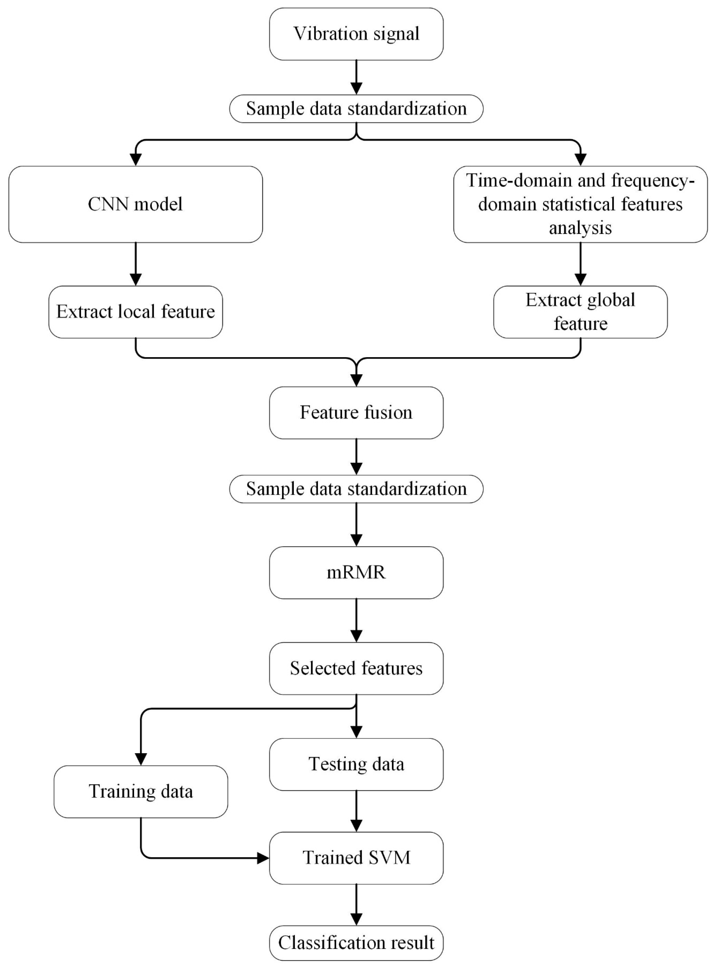
In GL-mRMR-SVM model, firstly, the global features from time-domain and frequency-domain statistical features are combined with the local features extracted by CNN from vibration signals. These global features can further enhance the model’s ability to identify different faults and make full use of the information in the raw data. It is worth noting that, in CNN, the extracted local features are not activated by the Softmax function. Then, the mRMR algorithm is used to automatically extract the discriminative features from the fused features without any prior knowledge. Through the mRMR algorithm, we can eliminate local features with poor robustness and global features that do not well characterize fault information. This will further improve the classification accuracy and reduce the training time of the model. Finally, the selected discriminative features are input into support vector machines (SVM). Although we introduce the handcrafted features into the proposed model, we do not need any prior knowledge due to the existence of feature selection algorithms. The architecture of the GL-mRMR-SVM model is shown in Figure 3.

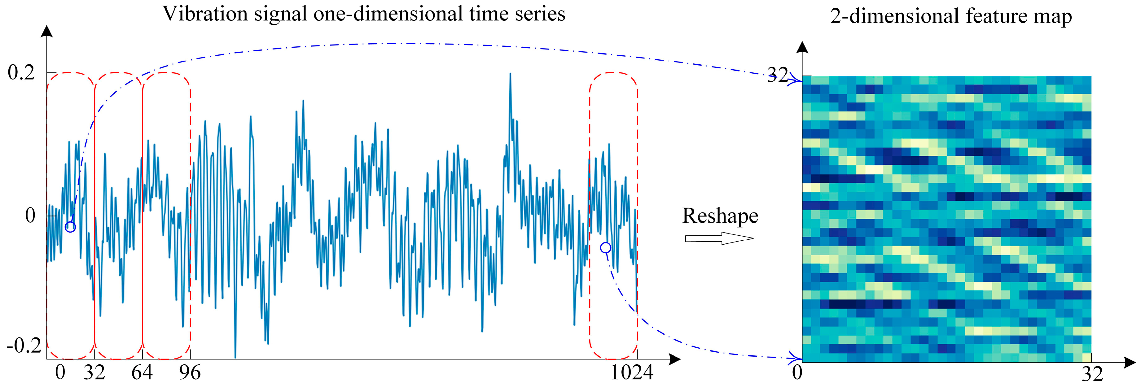
The CNN consists of one input layer, two convolution layers, two pooling layers, one fully connected layer, and one output layer (Figure 3). Dropout [27] is used after the pooling layer to prevent overfitting. The input of CNN is usually two-dimensional grid data or three-dimensional data [28]. A data reconstruction method that reconstructs one-dimensional time series of vibration signals into two-dimensional feature maps is used in this paper. Figure 4 shows the process of data reconstruction.

Table 1. GL-mRMR-SVM parameters.

CNN			SVM
Layers	Hyper-Parameter Settings	Training Parameters	The penalty factor C = 128; Kernel function is Gaussian Radial basis function (RBF); Kernel function parameters = 0.5
Input layer	32 × 32 inputs	Adam Batch size = 64 Learning rate = 0.003 Epoch = 20 Dropout = 0.3 (Ks is kernel size, Kn is kernel number, S is sub-sampling rate, N is number of hidden layer neuron nodes)
C1	Ks = 5 × 5, Kn = 32, Stride = 2, activation = ReLU
P2	S = 2
C3	Ks = 3 × 3, Kn = 64, Stride = 1, activation = ReLU
P4	S = 2
F5	N = 128, activation = ReLU
Output layer	The output is the number of classes, activation = Softmax

shows the detailed parameters of the GL-mRMR-SVM model.

As shown in Figure 3, the main parameters in GL-mRMR-SVM are m, n, and k. n is the number of categories. m affects the effect of the proposed method. The larger the m is, the more statistical features from time-domain and frequency-domain are candidates, the greater is the probability of occurrence of robust features, thus the more accurate are the results. However, as m increases, the computational capacity also increases. Fortunately, m does not need to be very large in most case if the value of k is appropriate. There is no accurate way to determine the value of k. However, when the statistical features from time-domain and frequency-domain inputted into the model are the same, the value of k is relatively determined for similar classification problems.

In GL-mRMR-SVM model, the forward and backward propagation of CNN is implemented by the CNN-Softmax model. Figure 5 shows the intelligent fault diagnosis process of the GL-mRMR-SVM model.

4. Experimental Evaluation

Experiments were carried out on the bearing data platform of CWRU to verify the robustness of the proposed method. The generalization of the proposed method was verified on the bearing data platform of CUT-2.

4.1. Robustness Experiment

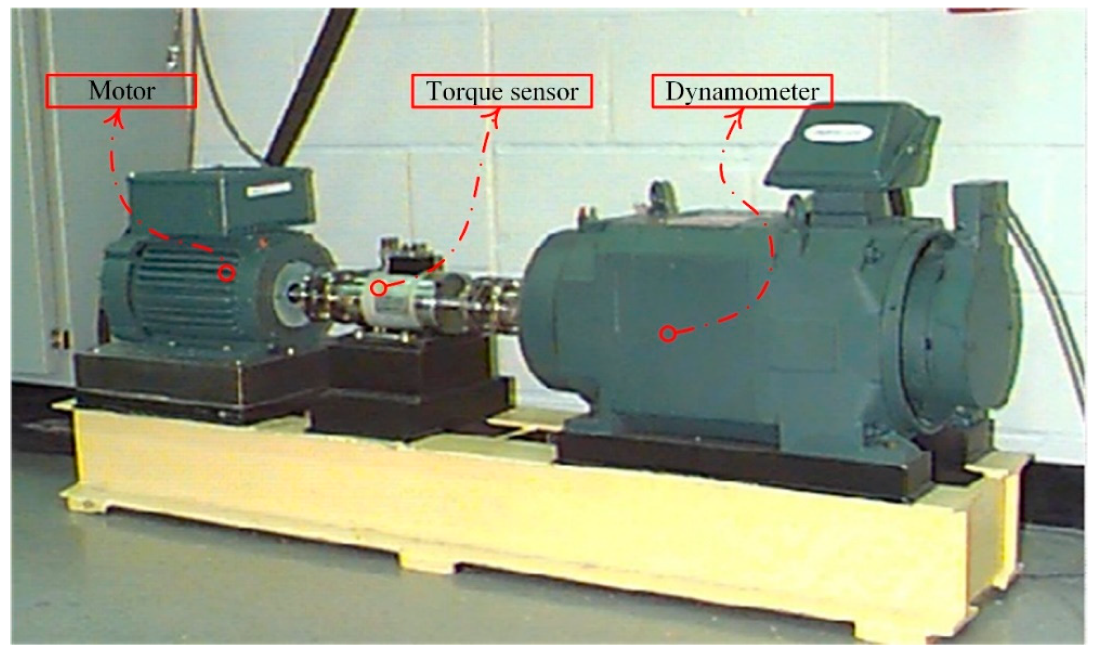
Open bearing data of CWRU were used for the experiment [29]. The experimental platform is shown in Figure 6. The left side of the diagram is a 1.5-kW motor, the middle is a torque sensor, and the right side is a dynamometer. The experimental bearing is 6205-2RS JEM SKF deep groove ball bearing, which was installed in the drive end of the motor housing to support the motor shaft.

The motor load is about 1 horsepower and the bearing speed is 1772 r/min. Single faults were placed on the inner race, the ball, and the outer race of the experimental bearing by electric discharge machining (EDM) technology. The diameter of faults were 0.007, 0.014, and 0.021 inches, respectively. The fault location of the outer race of the bearing was six o’clock and the sampling frequency was 12 K. The dataset size of each fault type was determined based on sampling without replacement, and the sampling length was set to 1024 unit. The specific experimental sample information is shown in

Table 2. Composition of CWRU experimental samples.

Fault Location	Fault Diameter (Inches)	Training	Testing	Condition Label
Normal	None	150	50	0
Inner Race	0.007	150	50	1
Ball	0.007	150	50	2
Outer Race	0.007	150	50	3
Inner Race	0.014	150	50	4
Ball	0.014	150	50	5
Outer Race	0.014	150	50	6
Inner Race	0.021	150	50	7
Ball	0.021	150	50	8
Outer Race	0.021	150	50	9

.

When a mechanical equipment fails, the probability distribution of its time-domain and frequency-domain signals change accordingly. Therefore, the fault information of mechanical equipment can be reflected by global features from time-domain and frequency-domain. The global features from time-domain and frequency-domain used in this work are shown in

Table 3. Global features in the time-domain and frequency-domain [30,31].

Features in Time-Domain		Features in Frequency-Domain
$f_0=\frac{{{\displaystyle \sum }}_{n=1}^{N}x\left(n\right)}{N}$	$f_6=\frac{{{\displaystyle \sum }}_{n=1}^N{\left(x\left(n\right)-f_0\right)}^4}{\left(N-1\right)f_2^4}$	$f_{12}=\frac{{{\displaystyle \sum }}_{k=1}^{K}s\left(k\right)}{K}$	$f_{19}=\sqrt{\frac{{{\displaystyle \sum }}_{k=1}^K{f}_k{}^{4}s\left(k\right)}{{{\displaystyle \sum }}_{k=1}^K{f}_k{}^{2}s\left(k\right)}}$
$f_1=\sqrt{\frac{{{\displaystyle \sum }}_{n=1}^N{\left(x\left(n\right)\right)}^2}{N-1}}$	$f_7=\frac{f_4}{f_3}$	$f_{13}=\frac{{{\displaystyle \sum }}_{k=1}^K{\left(s\left(k\right)-f_{12}\right)}^2}{K-1}$	$f_{20}=\sqrt{\frac{{{\displaystyle \sum }}_{k=1}^K{f}_k{}^{2}s\left(k\right)}{{{\displaystyle \sum }}_{k=1}^{K}s\left(k\right){{\displaystyle \sum }}_{k=1}^K{f}_k{}^{4}s\left(k\right)}}$
$f_2={\left(\frac{{{\displaystyle \sum }}_{n=1}^N\sqrt{\left|x\left(n\right)\right|}}{N}\right)}^2$	$f_8=\frac{f_4}{f_2}$	$f_{14}=\frac{{{\displaystyle \sum }}_{k=1}^K{\left(s\left(k\right)-f_{12}\right)}^3}{K{\left(\sqrt{f_{13}}\right)}^3}$	$f_{21}=\frac{f_{17}}{f_{16}}$
$f_3=\sqrt{\frac{{{\displaystyle \sum }}_{n=1}^N{\left(x\left(n\right)\right)}^2}{N}}$	$f_9=\frac{f_3}{\frac{1}{N}{{\displaystyle \sum }}_{n=1}^N\left|x\left(n\right)\right|}$	$f_{15}=\frac{{{\displaystyle \sum }}_{k=1}^K{\left(s\left(k\right)-f_{12}\right)}^4}{K{\left(f_{13}\right)}^2}$	$f_{22}=\frac{{{\displaystyle \sum }}_{k=1}^K{\left(f_k-f_{16}\right)}^{3}s\left(k\right)}{K{f}_{17}{}^3}$
$f_4=\max \left|x\left(n\right)\right|$	$f_{10}=\frac{f_4}{\frac{1}{N}{{\displaystyle \sum }}_{n=1}^N\left|x\left(n\right)\right|}$	$f_{16}=\frac{{{\displaystyle \sum }}_{k=1}^K{f}_{k}s\left(k\right)}{{{\displaystyle \sum }}_{k=1}^{K}s\left(k\right)}$	$f_{23}=\frac{{{\displaystyle \sum }}_{k=1}^K{\left(f_k-f_{16}\right)}^{4}s\left(k\right)}{K{f}_{17}{}^4}$
$f_5=\frac{{{\displaystyle \sum }}_{n=1}^N{\left(x\left(n\right)-f_1\right)}^3}{\left(N-1\right)f_2^3}$.	$f_{11}={\displaystyle {\displaystyle \sum }_{n=1}^N}{\left|x\left(n\right)\right|}^2$	$f_{17}=\sqrt{\frac{{{\displaystyle \sum }}_{k=1}^K{\left(f_k-f_{16}\right)}^{2}s\left(k\right)}{K}}$	$f_{24}=\frac{{{\displaystyle \sum }}_{k=1}^K{\left(f_k-f_{16}\right)}^{1/2}s\left(k\right)}{K\sqrt{f_{17}}}$
		$f_{18}=\sqrt{\frac{{{\displaystyle \sum }}_{k=1}^K{f}_k{}^{2}s\left(k\right)}{{{\displaystyle \sum }}_{k=1}^{K}s\left(k\right)}}$.
$x\left(n\right)$ is the time-domain signal sequence, $n=1,2,\dots ,N$, $N$ is the number of each sample points.		$s\left(k\right)$ is the frequency-domain signal sequence, $k=1,2,\dots ,K$, $K$ is the number of spectral lines.

.

In this experiment, m was set to be 25. k was chosen based on its uncertainty and importance. k was set to be 8, 10, 12, 14, 16, 18, and 20, respectively. The precision ratio p, recall ratio r, accuracy, and F1 measure f1 are used for model performance analysis, and their corresponding mathematical expressions are as follows:

$$\begin{array}{c}\{\begin{array}{c}\begin{array}{c}p = \frac{TP}{TP+FP}\\ r = \frac{TP}{TP+FN}\\ accuracy = \frac{TP+TN}{TP+FP+TN+FN}\end{array}\\ f1 = \frac{2}{\frac{1}{p}+\frac{1}{r}}\end{array}\end{array}$$

(10)

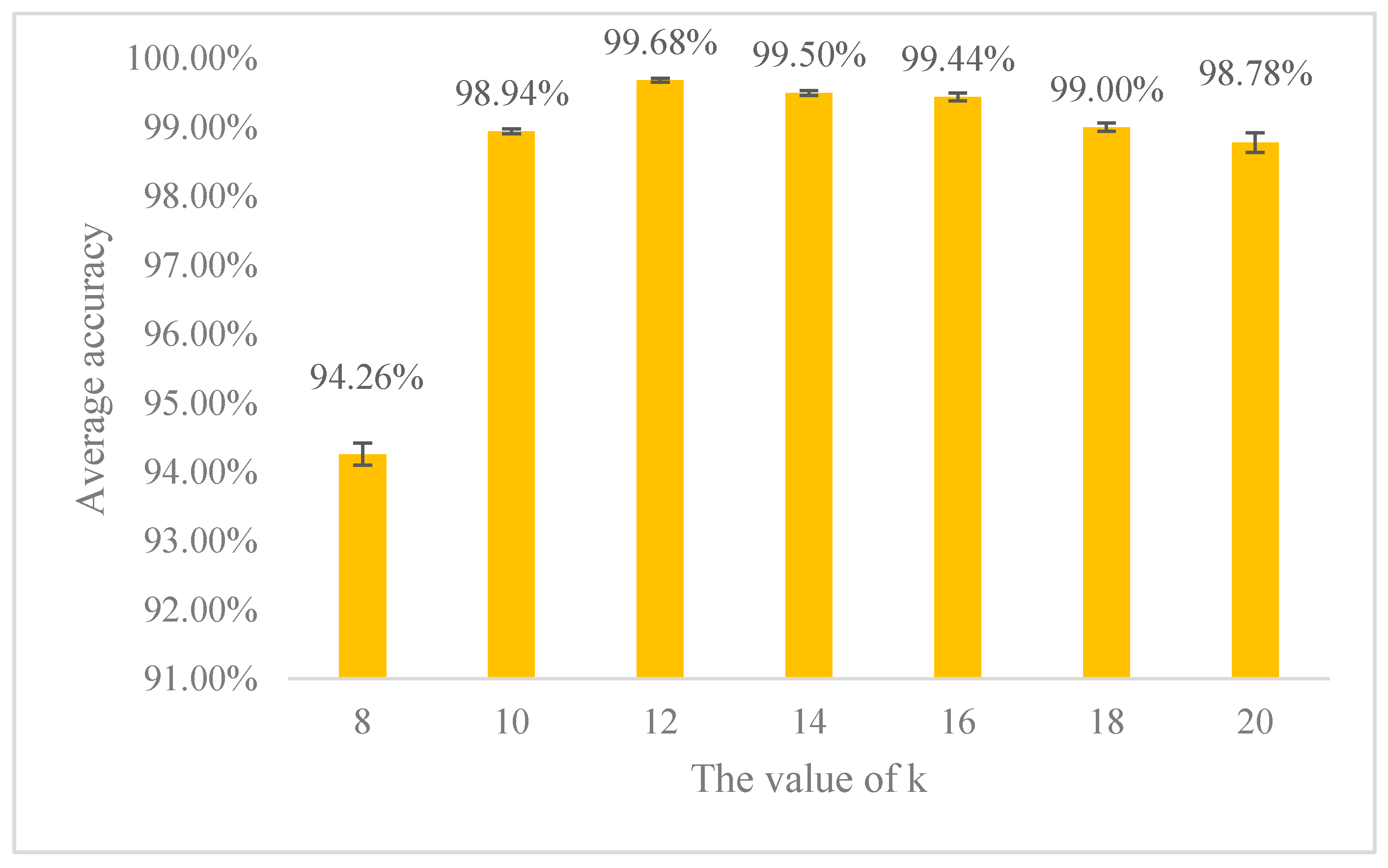
where TP is the number of true positive samples, TN is the number of true negative samples, FP is the number of false positive samples, and FN is the number of false negative samples. To rule out contingency, 10 random trials were performed for each model; all trials in this study used this standard. The average test accuracy and standard deviation of different values of k are illustrated in Figure 7.

First, as shown in Figure 7, GL-mRMR-SVM obtains similar results and excellent accuracy with different k values except k = 8. When k = 8, the average accuracy of the model is only 94.26%. The reason for this situation is that, when k = 8, the number of features selected is less than the dimension of CNN model output, which will inevitably lead to the loss of effective local features, and the global features that can represent fault information cannot be well utilized. When k ≥ 10, the average accuracy of the model is above 98.78%, which indicates that the proposed GL-mRMR-SVM model has excellent performance in fault diagnosis. In addition, Figure 7 also shows that the average accuracy of the model increases first and then decreases with the increase of k value. With the increase of k, the feature selection algorithm can select more discriminative features from the fused features, thus increasing the accuracy of the model. However, when k is increased to a certain extent, if k continues to increase, then the feature selection algorithm has to select some features with relatively poor robustness from the fused features. These indiscriminative features will inevitably lead to the decline of model accuracy. When k = 12, the average accuracy of the model reaches 99.68% and the standard deviation of accuracy reaches the minimum, which shows that the features selected by GL-mRMR-SVM have robustness.

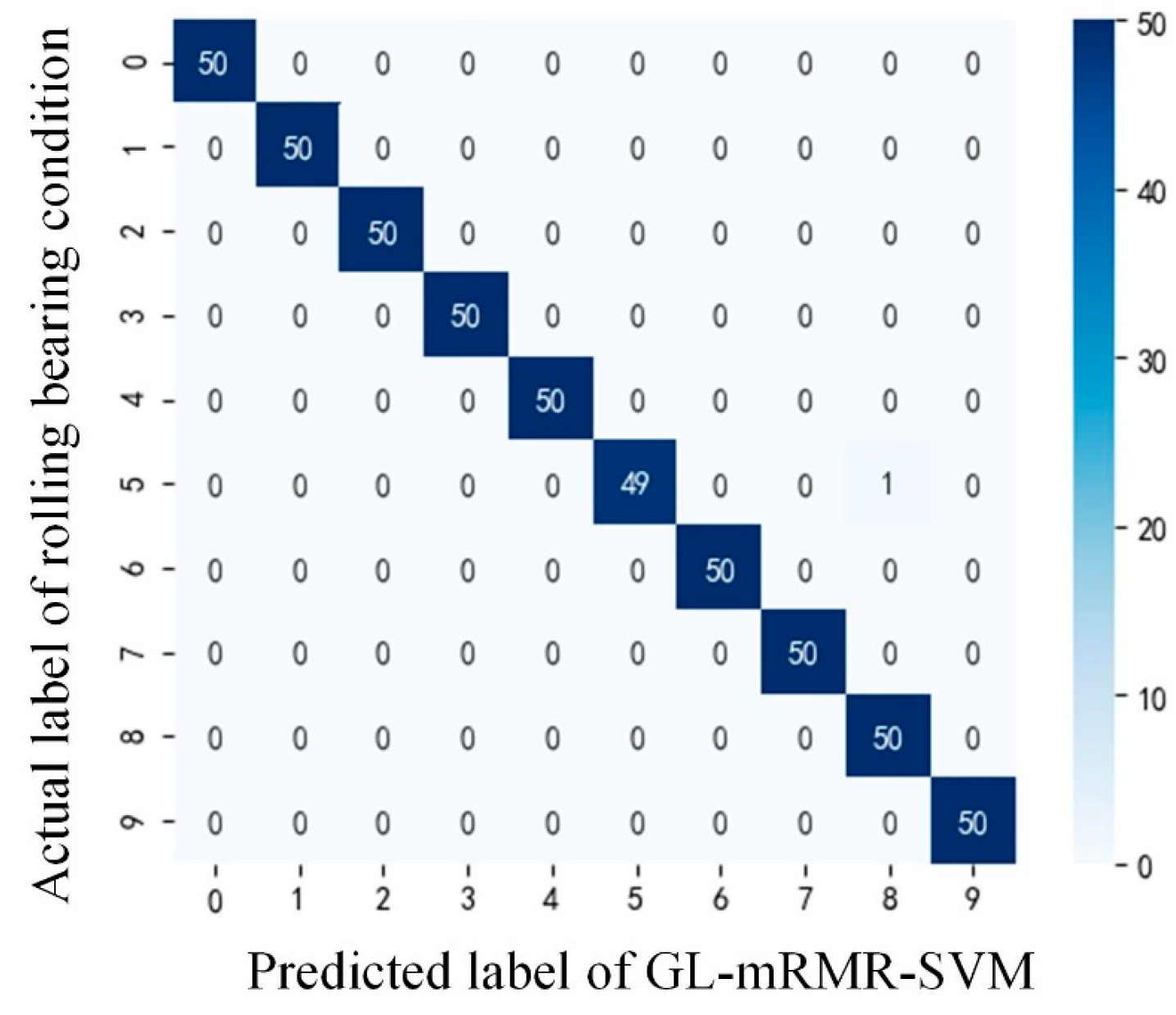
Considering comprehensively, k was determined to be 12 in this experiment.

Table 4. Test results of the proposed GL-mRMR-SVM model.

Condition Label	Precision Rate	Recall Rate	F1 Measure	Sample Amount
0	100%	100%	100%	50
1	100%	100%	100%	50
2	100%	100%	100%	50
3	100%	100%	100%	50
4	100%	100%	100%	50
5	100%	98.00%	98.99%	50
6	100%	100%	100%	50
7	100%	100%	100%	50
8	98.04%	100%	99.01%	50
9	100%	100%	100%	50
Average/Total	99.80%	99.80%	99.80%	500

lists the precision rates, recall rates, and f1 of the final experimental results of the proposed GL-mRMR-SVM method. In Table 4, the precisions of all labels except Label 8 are 100%. To further evaluate the classification of the faults of each type of GL-mRMR-SVM model, the confusion matrix is introduced for a detailed quantitative analysis. The confusion matrix shown in Figure 8 corresponds to the results in Table 4. In Figure 8, the x-axis andy-axis represent the labels predicted by GL-mRMR-SVM model and the actual labels of rolling bearing condition, respectively. Among 500 test samples, only one prediction result of GL-mRMR-SVM model is wrong. The actual label of the misclassified sample is 5 (Location: Ball; Diameter: 0.014), while the label predicted by GL-mRMR-SVM model is 8 (Location: Ball; Diameter: 0.021). Therefore, the model GL-mRMR-SVM is only likely to be confused when the severity of the fault is predicted.

To illustrate the superiority of GL-mRMR-SVM, two intelligent fault diagnosis algorithms were used for comparison: CNN and GL-SVM. The input of CNN was reconstructed vibration signal, and its parameters were consistent with the previous description. In GL-SVM, the input of the classifier SVM was a fusion feature that combines local features and global features.

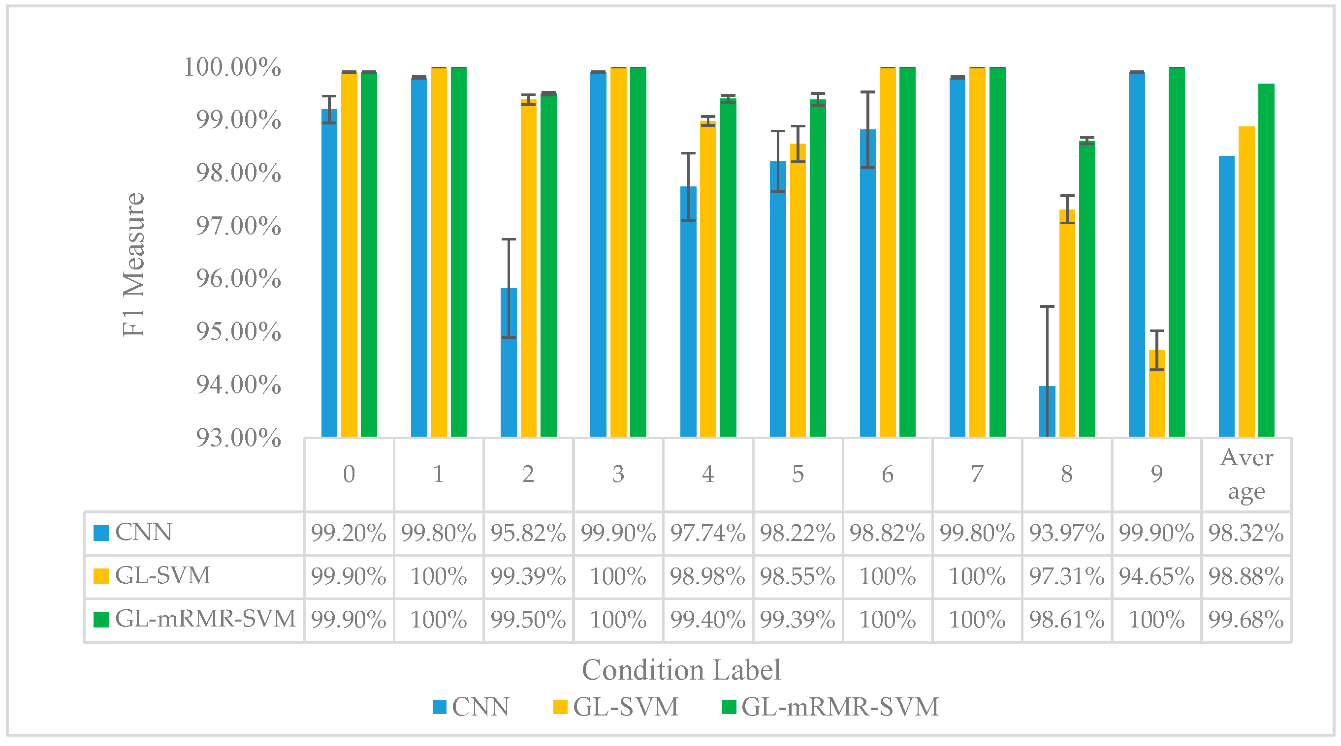
Comparing CNN with GL-mRMR-SVM can prove the effectiveness of introducing statistical features in time-domain and frequency-domain into bearing fault diagnosis. The advantages of feature selection can be highlighted by comparing GL-SVM with GL-mRMR-SVM. Because F1 measure is a commonly used comprehensive metric to measure the performance of a classification method, average value and standard deviation of F1 measure f1 was used as the evaluation metric of the model. The experimental results are presented in Figure 9, which shows that the proposed GL-mRMR-SVM has the best classification performance on each type of fault, with an average f1 score of 99.68%. Thus, the proposed GL-mRMR-SVM can learn more robust and discriminative features from vibration signals than others methods. It is worth mentioning that the GL-SVM model incorporating global features also performs well, which may be due to the less noise contained in the bearing data of CWRU, resulting in better robustness of global features.

In practical applications, the working environment of the bearing is usually complicated, and the measured bearing vibration signal also contains noise. For this reason, Gaussian white noise is added to the original signal to construct noise signals with different signal-to-noise ratios (SNR). SNR is defined as follows:

$$SN{R}_{dB}=10lo{g}_{10}\frac{p_{signal}}{p_{noise}}$$

(11)

where P_signal is the effective power of the signal and P_noise is the effective power of the noise.

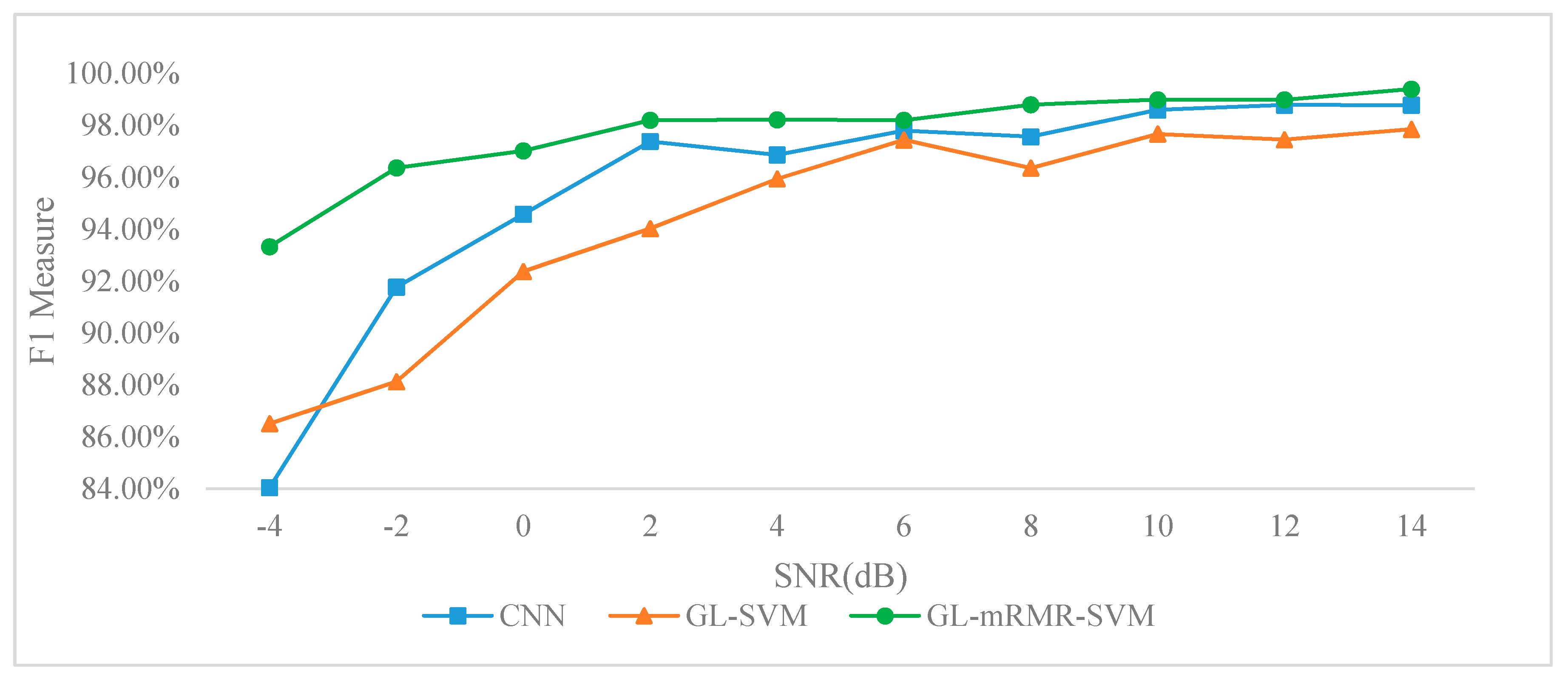
To further illustrate the robustness and reliability against noise of GL-mRMR-SVM, we used noisy signals with different SNRs from −4 to 14 dB to evaluate the proposed method. Figure 10 shows the evaluation results of CNN, GL-SVM, and GL-mRMR-SVM, where the average results of F1 measures for all ten conditions were calculated as the evaluation metric. It is clear that the proposed GL-mRMR-SVM significantly outperforms CNN and GL-SVM, with over 93% test performance in terms of F1 measure at all considered SNR levels. When the power of the noise is equal to that of the vibration signal, where SNR is 0 dB, the test performance of GL-mRMR-SVM is over 97%. Specifically, when SNR is greater than 0, the test performance of GL-mRMR-SVM even increases to 98% at a stable level. In short, the proposed GL-mRMR-SVM presents superior robustness against noisy situations, which means that GL-mRMR-SVM can select discriminative features from local features and global features. In addition, the performance of GL-SVM combined with global features does not perform as well as traditional CNN in noisy situations. This is because a large amount of noise is incorporated into the global features, which results in the performance degradation of the model.

4.2. Generalization Experiment

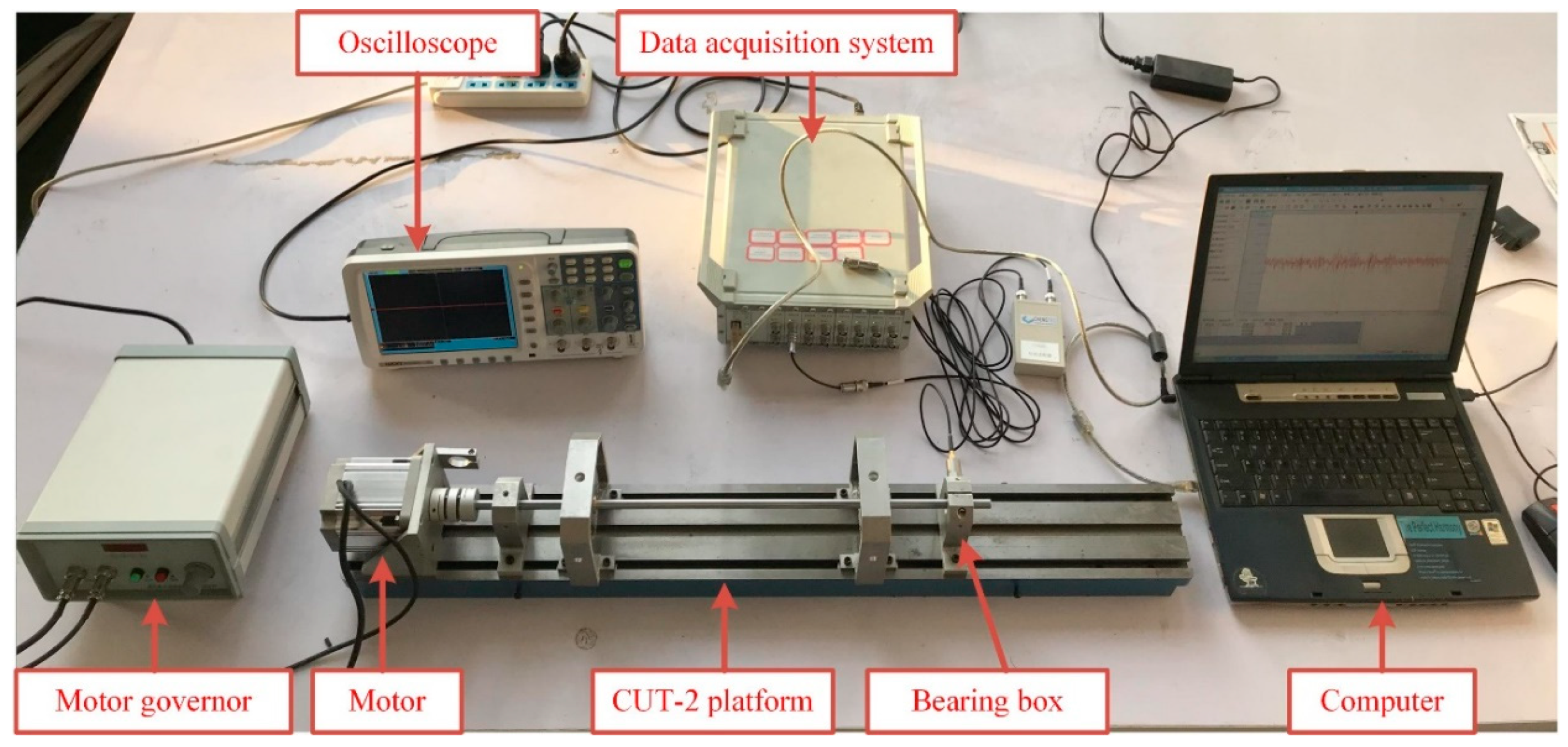
Composite fault recognition experiments were carried out on the bearing data platform of CUT-2 to verify the generalization performance of the proposed method. The bearing data platform of CUT-2 is shown in Figure 11. The experimental bearing is 6900ZZ deep groove ball bearing, and faults with diameters of 0.0787 and 0.1181 inches were arranged on the inner race, the ball, and the outer race of the experimental bearing by EMD technology. The location of the bearing faults is shown in Figure 12. The vibration signal of bearing compound fault was collected at the motor speed of 2000 r/min, the sampling frequency of 2K, and the sampling length of 1024. The specific experimental sample information is shown in

Table 5. Composition of CUT-2 experimental samples.

Compound Fault Location and Diameter			Training	Testing	Condition Label
Outer Race Fault Diameter (inches)	Inner Race Fault Diameter (inches)	Ball Fault Diameter (inches)
0.0787	0.0787	Null	150	50	0
0.1181	0.0787	Null	150	50	1
Null	0.0787	0.0787	150	50	2
Null	0.1181	0.0787	150	50	3
0.0787	Null	0.0787	150	50	4
0.0787	Null	0.1181	150	50	5
0.0787	0.0787	0.0787	150	50	6
0.0787	0.0787	0.1181	150	50	7

.

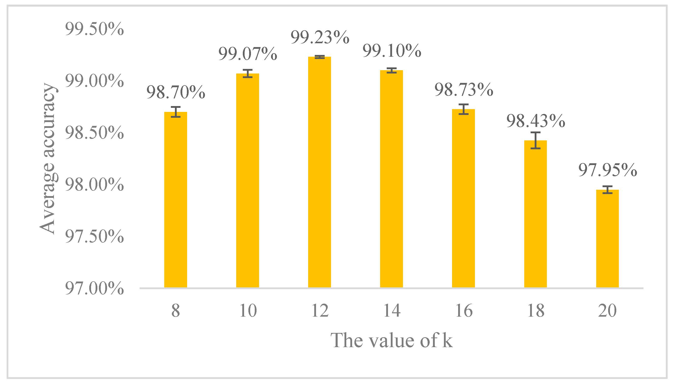
In this experiment, m was set to 25 as before, and k was set to 8, 10, 12, 14, 16, 18, and 20, respectively. The experimental results with different k are shown in Figure 13. The seven overall accuracies are all larger than 97.95% even if the fault is on different parts of the bearing at the same time. The performance of the GL-mRMR-SVM model is best when k = 12. As mentioned above, when the statistical features from time-domain and frequency-domain inputted into the model are the same, k does not change much for similar classification problems.

For comparison purposes, the CNN and GL-SVM models were compared with the proposed method, and the model parameters remained the same as described above. The results of different models according to F1 measure are shown in

Table 6. Experimental results with different models in term of F1 measure for each condition (%).

Condition Label	Models
	CNN	GL-SVM	GL-mRMR-SVM
0	97.88 ± 0.0243	97.53 ± 0.0266	98.40 ± 0.0085
1	97.89 ± 0.0556	99.59 ± 0.0046	99.60 ± 0.0024
2	99.03 ± 0.0201	90.97 ± 0.1292	99.41 ± 0.0024
3	96.15 ± 0.0388	95.49 ± 0.0347	98.70 ± 0.0141
4	98.66 ± 0.0308	98.77 ± 0.0189	99.80 ± 0.0016
5	99.12 ± 0.0104	99.60 ± 0.0045	99.70 ± 0.0021
6	96.43 ± 0.0538	97.83 ± 0.0277	98.48 ± 0.0174
7	99.40 ± 0.0064	99.49 ± 0.0047	99.70 ± 0.0041
Average	98.07	97.41	99.22

, and the classification results of each fault are shown. Table 6 shows that the average performance of the proposed GL-mRMR-SVM model for eight failures reaches 99.22%, which is better than the other two models. For each condition, GL-mRMR-SVM obtains the over 98.40% F1 measure, and a smaller standard deviation, which corresponds to more stable performance. In addition, the overall performance of GL-SVM is 97.41%, which is lower than the 98% of CNN. This is because the components of compound fault signal are complex, and some global features cannot well characterize the compound fault, thus the accuracy of the GL-SVM model integrated with global features decreases.

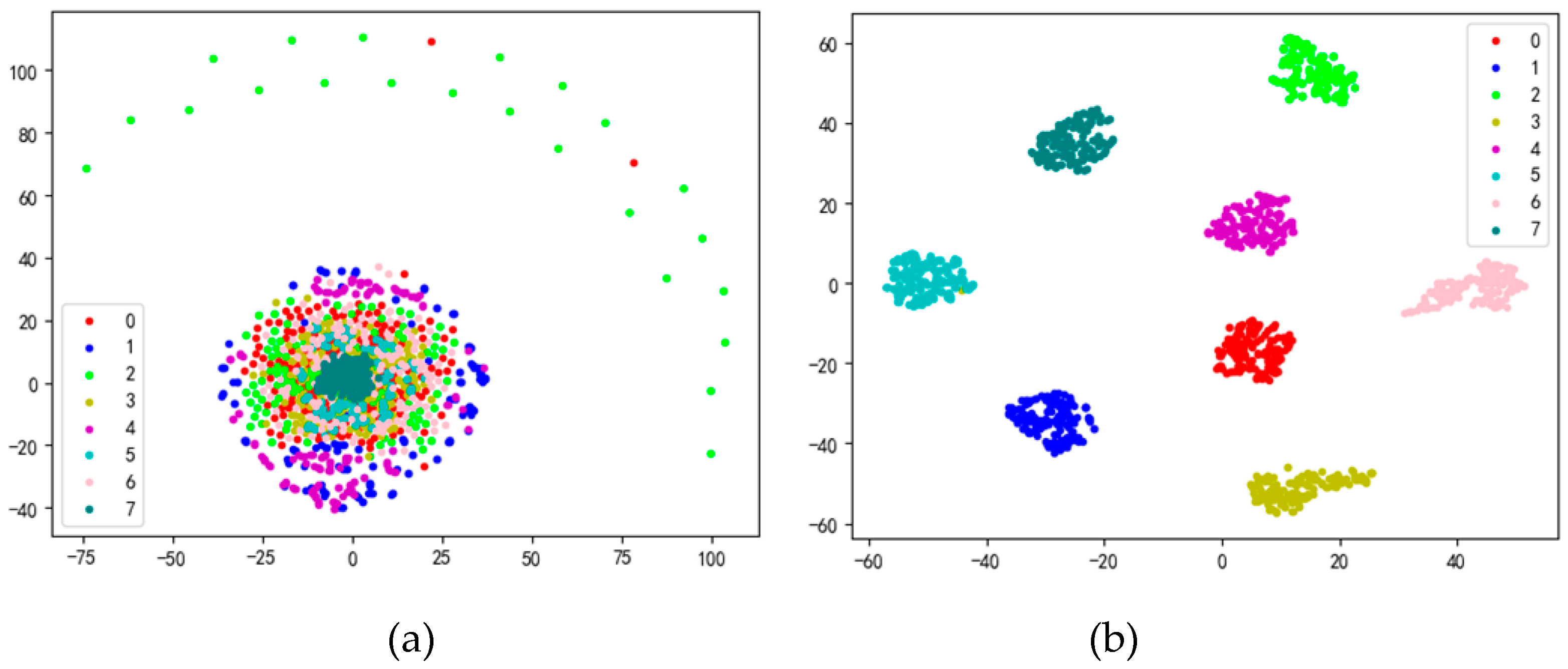
The t-distributed random neighborhood embedding (t-SNE) method of manifold learning was used for feature visualization to verify the learning ability of the proposed GL-mRMR-SVM for different compound fault categories. The feature visualization results of the raw samples and the extracted fusion feature are shown in Figure 14. As shown in Figure 14a, the eight categories of complex faults in the original sample are completely confused and difficult to distinguish between the categories. In Figure 14b, after feature fusion and feature selection of model GL-mRMR-SVM, eight samples of different categories are completely distinguished without intersecting the heterogeneous samples, which proves the good feature extraction ability of the model.

5. Conclusions and Future Work

A new framework (GL-mRMR-SVM) is presented for fault diagnosis of rolling bearing. Different from shallow classification models, which depend greatly on the handcrafted features and traditional deep learning models, the developed GL-mRMR-SVM system can combine the statistical features extracted from the time-domain and the frequency-domain with the local features extracted by the CNN, and the mRMR feature selection technique is used to extract discriminative features for model classification without any prior knowledge. The performance of the proposed GL-mRMR-SVM for single faults and compound faults was tested on CWRU and CUT-2 bearing datasets. The experimental results show that the proposed GL-mRMR-SVM model significantly outperforms the traditional deep learning model in terms of robustness against noise and classification performance, which is crucial for bearings that can make the mechanical system run steadily. More importantly, it provides a new idea and a general diagnostic framework for fault diagnosis, which can be easily extended to deal with different machines and industrial systems.

In future work, we will verify the scalability of the proposed GL-mRMR-SVM under different bearing experimental conditions, such as rotor unbalance and variable speed. In addition, the main parameters in GL-mRMR-SVM are m, n, k, and k, which decide the final results. There is no good way to optimize parameter k, which needs further research. However, for the same diagnosis object, the value of k is relatively certain, which we verified on two different bearing datasets.

References

1. Ciabattoni, L.; Ferracuti, F.; Freddi, A.; Monteriù, A. Statistical spectral analysis for fault diagnosis of rotating machines. IEEE Trans. Ind. Electron. 2018, 65, 4301–4310. [Google Scholar] [CrossRef]
2. Tra, V.; Kim, J.; Khan, S.A.; Kim, J.M. Bearing fault diagnosis under variable speed using convolutional neural networks and the stochastic diagonal Levenberg-Marquardt algorithm. Sensors 2017, 17, 2834. [Google Scholar] [CrossRef] [PubMed] [Green Version]
3. Lei, Y.; He, Z.; Zi, Y. Application of the EEMD method to rotor fault diagnosis of rotating machinery. Mech. Syst. Signal Process. 2009, 23, 1327–1338. [Google Scholar] [CrossRef]
4. Yan, R.; Gao, R.X.; Chen, X. Wavelets for fault diagnosis of rotary machines: A review with applications. Signal Process. 2014, 96, 1–15. [Google Scholar] [CrossRef]
5. Huang, N.E.; Shen, Z.; Long, S.R.; Wu, M.C.; Shin, H.H.; Zheng, Q.; Yen, N.-C.; Tung, C.C.; Liu, H.H. The empirical mode decomposition and the hilbert spectrum for nonlinear and nonstationary time series analysis. Proc. R. Soc. Lond. A Math. Phys. Eng. Sci. 1998, 454, 903–995. [Google Scholar] [CrossRef]
6. Lei, Y.; Zuo, M.J. Fault diagnosis of rotating machinery using an improved HHT based on EEMD andsensitive IMFs. Meas. Sci. Technol. 2009, 20, 125701. [Google Scholar] [CrossRef]
7. Yu, J. Local and nonlocal preserving projection for bearing defect classification and performance assessment. IEEE Trans. Ind. Electron. 2012, 59, 2363–2376. [Google Scholar] [CrossRef]
8. Liu, R.; Yang, B.; Zhang, X.; Wang, S.; Chen, X. Time–frequency atoms-driven support vector machine method for bearings incipient fault diagnosis. Mech. Syst. Signal Process. 2016, 75, 345–370. [Google Scholar] [CrossRef]
9. Chikalov, I.; Hussain, S.; Moshkov, M. Totally optimal decision trees for Boolean functions with at most five variables. In Procedia Computer Science; Elsevier Science Publishers: Amsterdam, The Netherlands, 2016. [Google Scholar]
10. Lecun, Y.; Bottou, L.; Bengio, Y.; Haffner, P. Gradient-based learning applied to document recognition. Proc. IEEE 1998, 86, 2278–2324. [Google Scholar] [CrossRef] [Green Version]
11. Liu, R.; Meng, G.; Yang, B.; Sun, C.; Chen, X. Dislocated time series convolutional neural architecture: An intelligent fault diagnosis approach for electric machine. IEEE Trans. Ind. Inform. 2017, 13, 1310–1320. [Google Scholar] [CrossRef]
12. Guoqian, J.; Haibo, H.; Jun, Y.; Xie, P. Multiscale convolutional neural networks for fault diagnosis of wind turbine gearbox. IEEE Trans. Ind. Electron. 2018, 66, 99. [Google Scholar]
13. Gong, W.; Chen, H.; Zhang, Z.; Zhang, M.; Wang, R.; Guan, C.; Wang, Q. A novel deep learning method for intelligent fault diagnosis of rotating machinery based on improved CNN-SVM and multichannel data fusion. Sensors 2019, 19, 1963. [Google Scholar] [CrossRef] [PubMed] [Green Version]
14. Huaqing, W.; Shi, L.; Liuyang, S.; Lingli, C. A novel convolutional neural network based fault recognition method via image fusion of multi-vibration-signals. Comput. Ind. 2019, 105, 182–190. [Google Scholar]
15. Liu, X.; Zhou, Q.; Zhao, J.; Shen, H.; Xiong, X. Fault diagnosis of rotating machinery under noisy environment conditions based on a 1-D convolutional autoencoder and 1-D convolutional neural network. Sensors 2019, 19, 972. [Google Scholar] [CrossRef] [PubMed] [Green Version]
16. Li, H.; Huang, J.; Ji, S. Bearing fault diagnosis with a feature fusion method based on an ensemble convolutional neural network and deep neural network. Sensors 2019, 19, 2034. [Google Scholar] [CrossRef] [PubMed] [Green Version]
17. Lu, W.; Liang, B.; Cheng, Y.; Meng, D.; Yang, J.; Zhang, T. Deep model based domain adaptation for fault diagnosis. IEEE Trans. Ind. Electron. 2016, 64, 99. [Google Scholar] [CrossRef]
18. Li, X.; Zhang, W.; Ding, Q. Understanding and improving deep learning-based rolling bearing fault diagnosis with attention mechanism. Signal Process. 2019, 161, 136–154. [Google Scholar] [CrossRef]
19. Abdeljaber, O.; Sassi, S.; Avci, O.; Kiranyaz, S.; Ibrahim, A.A.; Gabbouj, M. Fault detection and severity Identification of ball bearings by online condition monitoring. IEEE Trans. Ind. Electron. 2018, 66, 8136–8147. [Google Scholar] [CrossRef] [Green Version]
20. Xiaoan, Y.; Minping, J. Intelligent fault diagnosis of rotating machinery using improved multiscale dispersion entropy and mRMR feature selection. Knowl. Based Syst. 2018, 163, 450–471. [Google Scholar]
21. Hubel, D.H.; Wiesel, T.N. Receptive fields of single neurones in the cat’s striate cortex. J. Physiol. 1959, 148, 574–591. [Google Scholar] [CrossRef]
22. Hubel, D.H.; Wiesel, T.N. Receptive fields and functional architecture of monkey striate cortex. J. Physiol. 1968, 195, 215–243. [Google Scholar] [CrossRef] [PubMed]
23. Peng, H.; Long, F.; Ding, C. Feature selection based on mutual information: Criteria of max-dependency, max-relevance and min-redundancy. IEEE Trans. Pattern Anal. Mach. Intell. 2005, 27, 1226–1238. [Google Scholar] [CrossRef]
24. Li, B.; Zhang, P.-L.; Tian, H.; Mi, S.-S.; Liu, D.-S.; Ren, G.-Q. A new feature extraction and selection scheme for hybrid fault diagnosis of gearbox. Expert Syst. Appl. 2011, 38, 10000–10009. [Google Scholar] [CrossRef]
25. Jin, X.; Ma, E.W.M.; Cheng, L.L.; Pecht, M. Health monitoring of cooling fans based on mahalanobis distance with mRMR feature selection. IEEE Trans. Instrum. Meas. 2012, 61, 2222–2229. [Google Scholar] [CrossRef]
26. Li, Y.; Yang, Y.; Li, G.; Xu, M.; Huang, W. A fault diagnosis scheme for planetary gearboxes using modified multi-scale symbolic dynamic entropy and mRMR feature selection. Mech. Syst. Signal Process. 2017, 91, 295–312. [Google Scholar] [CrossRef]
27. Srivastava, N.; Hinton, G.; Krizhevsky, A.; Sutskever, I.; Salakhutdinov, R. Dropout: A simple way to prevent neural networks from overfitting. J. Mach. Learn. Res. 2014, 15, 1929–1958. [Google Scholar]
28. Noda, K.; Yamaguchi, Y.; Nakadai, K.; Okuno, H.G.; Ogata, T. Audio-visual speech recognition using deep learning. Appl. Intell. 2015, 42, 722–737. [Google Scholar] [CrossRef] [Green Version]
29. Lou, X.; Loparo, K.A. Bearing fault diagnosis based on wavelet transform and fuzzy inference. Mech. Syst. Signal Process. 2004, 18, 1077–1095. [Google Scholar] [CrossRef]
30. Tang, X.; Wang, J.; Lu, J.; Liu, G. Improving bearing fault diagnosis using maximum information coefficient based feature selection. Appl. Sci. 2018, 8, 2143. [Google Scholar] [CrossRef] [Green Version]
31. Lei, Y.; He, Z.; Zi, Y. Fault diagnosis based on novel hybrid intelligent model. Chin. J. Mech. Eng. 2008, 44, 112–117. [Google Scholar] [CrossRef]
Figure 1. A typical architecture of CNN.
Processes 08 00784 g001
Figure 2. Single Convolutional Neural Network.
Processes 08 00784 g002
Figure 3. Schematic diagram of GL-mRMR-SVM.
Processes 08 00784 g003
Figure 4. The process of data reconstruction.
Processes 08 00784 g004
Figure 5. The intelligent fault diagnosis process of GL-mRMR-SVM model.
Processes 08 00784 g005
Figure 6. CWRU bearing experimental platform.
Processes 08 00784 g006
Figure 7. Accuracy and standard deviation of different k values.
Processes 08 00784 g007
Figure 8. GL-mRMR-SVM results when k = 12.
Processes 08 00784 g008
Figure 9. Diagnosis result on the testing set using different methods.
Processes 08 00784 g009
Figure 10. Diagnosis result on noisy signals with different SNRs using CNN, GL-SVM, and the proposed GL-mRMR-SVM.
Processes 08 00784 g010
Figure 11. CUT-2 bearing experimental platform.
Processes 08 00784 g011
Figure 12. The location of the bearing faults: outer race fault (a); inner race fault (b); ball fault (c); and combination of parts (d).
Processes 08 00784 g012
Figure 13. GL-mRMR-SVM results with different k under compound fault.
Processes 08 00784 g013
Figure 14. Feature visualization of compound fault: (a) the raw samples; and (b) the extracted fusion.
Processes 08 00784 g014