Model-Based Process Optimization for the Production of Macrolactin D by Paenibacillus polymyxa

Abstract

In this study, we show the successful application of different model-based approaches for the maximizing of macrolactin D production by Paenibacillus polymyxa. After four initial cultivations, a family of nonlinear dynamic biological models was determined automatically and ranked by their respective Akaike Information Criterion (AIC). The best models were then used in a multi-model setup for robust product maximization. The experimental validation shows the highest product yield attained compared with the identification runs so far. In subsequent fermentations, the online measurements of CO₂ concentration, base consumption, and near-infrared spectroscopy (NIR) were used for model improvement. After model extension using expert knowledge, a single superior model could be identified. Model-based state estimation with a sigma-point Kalman filter (SPKF) was based on online measurement data, and this improved model enabled nonlinear real-time product maximization. The optimization increased the macrolactin D production even further by 28% compared with the initial robust multi-model offline optimization.

1. Introduction

Process monitoring based on mechanistic nonlinear models combined with atline and online measurement data [1,2,3,4,5,6,7,8] enables the detection of undesired deviations over the course of fermentations. This kind of process intelligence is promoted by the Process Analytical Technology (PAT) initiative defined by the United States Food and Drug Administration (FDA) [9,10]. With increased precision and availability, Raman [11,12,13] and near-infrared (NIR) [13,14,15,16,17] spectroscopy are used more often in recent years for cultivation monitoring. Most of the time, a partial least squares regression (PLS) is used for multivariate data analysis to correlate the analyte, for example, biomass or glucose concentration in the cultivation broth, with the spectroscopic information contained in the spectra. In contrast to process spectroscopy, a nonlinear process model enables model-predictive control or real-time optimization of processes. This has successfully been applied for chemical processes [18] and is an established state-of-the-art method in chemical industry [19]. However, fewer examples of its application in the biotechnological sector have been published so far [1,20,21,22,23,24,25]. One of the very first applications in which the production of an antibiotic by a mycelial organism was optimized was reported in 1993 [26,27,28].

Some authors have performed offline optimization of fed-batch cultivations [29], but many focus on model-free process improvements [30] or model-free response surface optimizations using a classical design of experiments [31]. The biggest obstacle for the use of model-based approaches is the effort of obtaining a suitable biological process model. A possible solution is the automation of this step to facilitate the use of model-based methods. The approach published by Herold and King [32] can be used to automatically generate structured models of low complexity based on measurement data. After interpolation of all the measured quantities in a cultivation, their change over time is merged in a few distinctive phenomena that are then compared to assign probabilities to model components for example limiting behavior of a substrate. As a result, a family of process models with a descending probability can be created in the form of differential equations in MATLAB code, and their respective model parameters can be estimated using automated code generation [33].

The organism Paenibacillus polymyxa (P.p.), which is used as an example in the current case study, produces macrolactin D under limiting conditions. Macrolactins are of interest because of their antibacterial and, in some cases, antiviral effects [34,35]. For further information, see [36]. Other use cases of P.p. are the production of enhanced 2,3-Butanediol. For this application, Okonkwo et al. [37] performed model-free optimization via response-surface methodology. A very basic model of P.p. was developed by Haughney and Nauman [38], which cannot necessarily be transferred to other strains of the organism. For the strain of P.p. used in this publication, a structured model was manually developed by Violet et al. [39]. Due to the high number of parameters, the identifiability of this model is rather poor. In contrast to the fact that the model is very sophisticated, the dynamics of the macrolactin production could not be captured correctly.

In this publication, a different approach was chosen. The basic model was not developed manually, but via the automated model identification approach presented by Herold [40]. In this publication, we show how such models can successfully be used for robust optimization. On top of that, we show that this model provides a good basis for model improvement and extension. The refined model is the first published structured model of small size of P.p. that includes a model for the off-gas concentration and the base consumption. In conclusion, we show that the attained model quality is satisfactory for state estimation and online optimization. Besides a publication that uses P.p. as an example for cultivation monitoring via flourescence [41], this is the first publication that applies NIR-spectrsocopy to P.p. and furthermore integrates the results in a model-based state estimator.

The current paper is organized as follows: After a description of the experimental setup in Section 2.1, a general model is introduced in Section 2.2 with a discussion of various uncertainties, i.e., measurement, parameter, and model uncertainties. Multivariate analysis based on NIR data and model-based process optimization are discussed in Section 2.3 and Section 2.4, respectively. Optimization is divided up into an offline phase, named trajectory planning, and an online optimization. For optimization, a situation is considered in which a family of possible models is available. A state estimation using a sigma-point Kalman filter is summarized in Section 2.5 before the results of an online optimization and a discussion are presented in Section 3.

2. Materials and Methods

2.1. Experimental Setup

The experiments were performed at the Chair of Measurement and Control at Technische Universität (TU) Berlin using a wild-type strain Paenibacillus polymyxa capable of producing macrolactin D. The preculture protocol that was used for the cultivation of P.p. is given in [39]. The fermentations were carried out in a 22 L cultivation vessel (Biostat C, B. Braun Biotech Inc., Melsungen, Germany) initially containing 10.5 L chemically defined medium.

The feeding rates of the fed-batch cultivations were realized by proportional-integral-controlled pump-scale systems and can be altered online via a custom-made process control system based on a central mySQL database [33]. A gas analyzer (BlueInOne Cell, BlueSens gas sensor GmbH, Herten, Germany) was used to determine the off-gas fraction of CO₂. The pH value was measured using a glass electrode (405-DPAS-SC-K8S pH probe, Mettler-Toledo International Inc., Columbus, OH, USA) and controlled using sodium hydroxide and sulfuric acid to maintain a constant pH value of 7. The level of dissolved oxygen (InPro 6800, Mettler-Toledo International Inc., Columbus, OH, USA) was held at a minimum level of 50% by a PI controller that uses a stirrer speed with a minimum of 200 rpm at a sparging rate of 10 slm. The temperature was held constant at 28 °C. In the last four experiments, NIR spectra were recorded and processed online using a PGS 1.7 tc 512 (tec5 AG, Oberursel, Germany) equipped with the transmission probe Excalibur 12 (Hellma GmbH, Mullheim, Germany) with 1 mm gap width. The integration time of the sensors in the NIR spectrometer was 36 ms. Every 3 s, a spectrum was recorded and then pretreated and subsampled to a sampling frequency of $\frac{1}{6}{\min }^{-1}$. The same sampling frequency was applied for the off-gas carbon dioxide concentration and base consumed for pH control.

Substrate concentrations in the cultivation broth were determined photometrically using commercial enzyme kits (phosphate FS and glucose GOD FS, DiaSys Diagnostic Systems GmbH, Holzheim, Germany) and using the Berthelot reaction [42] for ammonium, here by applying fourfold determination in each case. The quantity of the product macrolactin D was determined via HPLC. The composition of the mobile phase changed linearly in 15 min from 100% of an aqueous solution of 0.1%H₃PO₄ to 100% acetonitril and after 2 min again in a linear gradient over 4 min back to 100% of an aqueous solution of 0.1%H₃PO₄. With the precolumn LiChrospher 100 RP-19 (5 μm) endcapped and the main column LiChrospher 100 RP-19 (5 μm), both made by Merck KGaA (Darmstadt, Germany), the retention time of macrolactin D was ca. 7.4 min at a detection wavelength of 230 nm (Detector PDA-100, Dionex Corporation, Sunnyvale, CA, USA).

Processing of samples, with the exception of the biomass, was conducted after the end of the batch. The biomass was determined twofold through filtering a defined volume of broth through a preweighed 0.2 μm filter, rinsing with water, drying, and dividing the difference in filter weight through the filtered volume.

2.2. Mathematical Fermentation Modeling

The automatic model building tool by Herold and King [32] creates model equations in the form of

$${\dot{m}}_i=u_i-q_{\mathrm{out}}+\sum _k\left(Y_k·\Pi r_j·P\left(m_i\right)\right),$$

(1)

where the mass $m_i$ denotes the states. For the state of a substrate, $u_i$ represents the feeding rate and $q_{\mathrm{out}}$ the loss because of manual sampling, where the sampling volume is drawn within a few seconds. The yield coefficients $Y_k$ describe how much substrate is needed for a unit of a respective reaction product. The formal kinetics $r_j$ describe the influence of the component’s concentrations to the respective reaction. Finally, the proportional factor $P(m_i)$, for example, the total biomass, scales the specific reaction rate to an absolute reaction rate. Three different model types can be differentiated: unstructured models with substrates and a single biotic state biomass, structured models of small size permitting internal storage compartments and an active biomass, and finally structured models of medium size using the cell-intern mass of DNA, RNA, proteines, amino acids, and nucleotides as states. Structured models of small size were used for their good trade-off between model complexity and predictive capacity. All models were assumed to be nonsegregated, meaning that the composition of the biomass is the same for all cells.

2.2.1. Measurement Uncertainty

The measurement uncertainty is of interest because it is used for parameter identification via a maximum-likelihood estimation (see [43]), for model discrimination and in the state estimation. In contrast to the established approaches, the uncertainty was assumed to depend on the value of the measurement of the component $i_y$ at time $i_t$, as in Equation (2). The linear structure results from experimental investigations with a large number of measurements and covers all kinds of errors such as absolute inaccuracies in the measuring instruments and relative inaccuracies in dilution series.

$${\sigma }_{i_t,i_y}=a_{i_y}{y}_{i_t,i_y}+b_{i_y}$$

(2)

The coefficients $a_{i_y}$ and $b_{i_y}$ were determined based on the method created by Heine et al. [44] and are given in

Table 1. Coefficients to describe the measurement uncertainty according to Equation (2).

	b in g/L					b in %	b in mL
	X	Am	Ph	C	Ml	CO2	Base
a in %	3	5.9	3.7	2.6	3.1	2	2
b	0.03	0.004	0.02	0.202	0.004	0.3	3

for the concentration of biomass (X), ammonium (Am), phosphate (Ph), glucose (C), macolactin (ML), as well as the carbon dioxide (CO₂) fraction in the off-gas, and the volume of added base.

2.2.2. Parameter Uncertainty

The examination of the parameter uncertainty is a valuable tool for assessing the predictive capacity of a model. The covariance matrix of the parameters ${\mathbf{C}}_{\underline{\theta }\underline{\theta }}$ can be approximated by the inverse of the Fisher information matrix F, which is a lower bound to ${\mathbf{C}}_{\underline{\theta }\underline{\theta }}$ [43]

$${\mathbf{C}}_{\underline{\theta }\underline{\theta }}\ge {\mathbf{F}}^{-1}={\left(\sum _{k=1}^{n_{\mathrm{sample}}}{\mathbf{F}}_k\right)}^{-1}.$$

(3)

The Fisher information matrix of a measurement i is as follows:

$${\mathbf{F}}_i=\left[{\left(\frac{d\underline{y}}{d\underline{\theta }}\right)}^T{\mathbf{C}}_{\underline{y}\underline{y}}^{-1}\left(\frac{d\underline{y}}{d\underline{\theta }}\right)\right]$$

(4)

with a diagonal covariance matrix of measurements ${\mathbf{C}}_{\underline{y}\underline{y}}$ based on Equation (2). The output sensitivities $\frac{d\underline{y}}{d\underline{\theta }}$ can be obtained by integrating the sensitivity differential equations [45] or, as it is done here, by using orthogonal collocation as differential equation solver, which allows us to explicitly determine the sensitivities S in parallel to the integration of the system differential equation [46]. The output sensitivities needed in Equation (4) are then readily derived.

2.2.3. Model Uncertainty

The parameter uncertainty represented by ${\mathbf{C}}_{\underline{\theta }\underline{\theta }}$ can only poorly map the error of a false model structure. Thanks to the modelling framework developed by Herold and King [32], various model structures were available to provide a similarly good description of the experiments after an automated and optimized parameter identification, here by using the methods of Violet [47]. This has to be pointed out because the optimized feeding profiles determined below will drive the system into regions where the model outputs actually differ significantly even though all the models could explain the first set of identification experiments equally well. This situation is often seen when approximative models are used to describe a biological system instead of exactly describing the complete metabolism of an organism, which is mostly impossible. According to Hurvich et al. [48] the Akaike’s information criterion (AIC) [49] with the correction for a small number of measurements (AIC_c) can be used for discrimination between such models. The model with the smallest AIC_c shows the best fit. Based on the distance to it, all m models can be evaluated, and model “probabilities” $w_{\mathrm{k}}$ can be deducted.

$$w_{\mathrm{k}}=\frac{exp\left(-\frac{{\Delta }_k}{2}\right)}{{\sum }_{\mathrm{j}=1}^{\mathrm{m}}exp\left(-\frac{{\Delta }_j}{2}\right)}\mathrm{with}{\Delta }_{\mathrm{k}}={\mathrm{AIC}}_{\mathrm{c},\mathrm{k}}-{\mathrm{AIC}}_{\mathrm{c},\min }$$

(5)

The use of the AIC is based on the assumptions that the correct model exists in the model family. Therefore, it should only be used as an indication as no “real” model exists here. Nevertheless, the model probabilities calculated in this way can be used as a first approximation for the multi-model approach of process optimization.

2.2.4. Parameter Subset Selection

Not all parameters in nonlinear biological models are easily identifiable. The parameter subset selection enables a reduction of the number of examined parameters. One way to reduce it is to use the singular value decomposition [50,51] to ensure an invertible Fisher information matrix at any time. The affected parameters are kept at the identified value, but their uncertainty is not considered further because they are not sensitive, i.e., they have no significant effect on the process. In the cases occurring here, an inversion of F was still possible but with great uncertainties. A parameter-centered approach considers the root of the diagonal elements of ${\mathbf{C}}_{\underline{\theta }\underline{\theta }}$, i.e., the standard deviation ${\underline{\sigma }}_{\underline{\theta }}$. By excluding extremely safe parameters and extremely unsafe parameters through deleting the corresponding rows and columns from F, the condition number of F was improved. The bounds were set to 5000% of the parameter value as the upper bound and 0.01% of the parameter value as the lower bound. The reduced parameter covariance matrix ${\mathbf{C}}_{\underline{\theta }\underline{\theta }}$ was then used for state estimation, as described below.

2.3. Multivariate Analysis of NIR Spectroscopy

For the data analysis, the python framework SciPy [52] was used. The NIR probe was placed directly in the agitated and aerated fermentation broth. To reduce the influence of gas bubbles and particle agglomerates, bubble detection was performed on all spectra. Equivalent to outlier detection [53], a modified z-score

$$M=\frac{x-\tilde{x}}{\tilde{\Delta }},$$

(6)

was defined, where $\tilde{x}$ is the median of the raw values x and $\tilde{\Delta }$ is the median of all deviations $\tilde{\Delta }=\mathrm{median}(x-\tilde{x}$). All measurements with $M>2.5$ were rejected. The methodology can be extended to a time series using the moving median $\tilde{x}(t)$ and $\tilde{\Delta }(t)$, where a span of 71 values is employed. Two separate wavelength areas were relevant for the calculation of M. The average of the raw values between the wavelengths of 1418 nm and 1432 nm was used for the detection of gas bubbles, and the range 1014–1279 nm was used for the detection of particle agglomerates. The remaining sensor raw values were then smoothed over the wavelength using Whittaker’s smoother [54] with a smoothing parameter of 0.01 filtered over time via acausal moving average with a span of 71 values and subsampled to a sampling frequency of $\frac{1}{6}{\min }^{-1}$. The median span, as well as, the chosen wavelengths and value of M depend on the NIR-data obtained and were used as tuning parameters. In general one has to define the correct values on a case-by-case basis to capture all the important phenomena and dynamics while eliminating noise and outliers.

Using a reference spectrum $I_0$, taken with demineralized water at 28 °C, the vector of the absorption $\underline{A}$ was calculated using the vector of sensor raw values (intensity) $\underline{I}$.

$$\underline{A}=-log(\underline{I})+log({\underline{I}}_0)$$

(7)

At low substrate concentrations and in the absence of particular substance, the absorption $\underline{A}$ is proportional to the concentration of the absorbing components in the sample [55]. Based on this assumption, a linear model in the form of $y={\underline{A}}^{\mathrm{T}}·\underline{\beta }$ can be postulated to predict the concentration y of the relevant components. The high correlation within the observed variables, here the spectrum $\underline{A}$, makes it almost impossible to use an ordinary linear regression. The widely applied partial least squares (PLS) regression using a matrix decomposition is well suited for this task. Here, the implementation within Python Scikit [56] was employed. A relevant meta-parameter is the number of factors, which is similar to the number of components when using a principal component regression. For cross-validation, the data set was randomly split up into six parts. Five of them were used for PLS regression with the number of factors ranging from 1 to 10, and the remaining part was used for validation. This was repeated five times until all measurements had been used for validation. This approach was repeated 10 times with different random splits. Based on the root mean square error of validation estimated this way, the number of factors could be determined to achieve a good match while avoiding overfitting.

The use of sample normalization (standard normal variate), as well as the use of derivatives obtained via Savitzky Golay filtering [57], had been rejected because it did not lead to superior regression performance.

2.4. Process Optimization

The constrained SQP algorithm SNOPT7 by Tomlab [58,59] was used for all optimization tasks. The general problem for the process optimization is given as:

$$\begin{array}{cc}\hfill \left\{{\underline{x}}_0,\underline{u}(t)\right\}& =arg\underset{{\underline{x}}_0,\underline{u}(t)}{min}\Phi \hfill \end{array}$$

(8)

$$\begin{array}{cc}\hfill \mathrm{s}.\mathrm{t}.:& \dot{\underline{x}}=\underline{f}(\underline{x}(t),\underline{u}(t),\underline{\theta }),\underline{x}\left(t_0\right)={\underline{x}}_0\hfill \end{array}$$

(9)

$$\begin{array}{cc}\hfill & {\underline{u}}_{min}\le \underline{u}(t)\le {\underline{u}}_{max}\hfill \end{array}$$

(10)

$$\begin{array}{cc}\hfill & {\underline{x}}_{min}\le \underline{x}(t)\le {\underline{x}}_{max}\hfill \end{array}$$

(11)

with an appropriate cost function $\Phi$. The feeding rates of phosphate (Ph), ammonium (Am), and glucose (C) at a constant feed concentration u(t) served as the optimization variables. The initial conditions were not subject to optimization here.

2.4.1. Robust Planning

As long as it is not possible to differentiate sufficiently well between a set of identified models, all of the respective models should be included in the process optimization. There are different approaches for considering multiple models in a process optimization. The MinMax criterion [60] improves the worst result of all the models.

$$\left\{{\underline{x}}_0,\underline{u}(t)\right\}=arg\underset{{\underline{x}}_0,\underline{u}(t)}{min}\underset{\mathrm{model}}{max}{\Phi }_k$$

(12)

where individual cost functions ${\Phi }_k$ are calculated for $n_k$ considered models. This approach focuses very strongly on the worst model. A less conservative result is obtained via the weighted sum of the results of all models. The model probability from the AIC can be taken into account for calculating this mean value. A complete failure of the experiments is prevented by the fact that the constraints have to be met for all the models. The optimization problem with the weights $w_k$ of the respective model k results in the following task:

$$\begin{array}{cc}\hfill \left\{{\underline{x}}_0,\underline{u}(t)\right\}& =arg\underset{{\underline{x}}_0,\underline{u}(t)}{min}\sum _{k=1}^{n_k}{w}_k{\Phi }_k\hfill \end{array}$$

(13)

$$\begin{array}{cc}\hfill \mathrm{s}.\mathrm{t}.:& {\dot{\underline{x}}}_k={\underline{f}}_k({\underline{x}}_k(t),\underline{u}(t),{\underline{\theta }}_k),\underline{x}\left(t_0\right)={\underline{x}}_0\hfill \end{array}$$

(14)

$$\begin{array}{cc}\hfill & {\underline{u}}_{min}\le \underline{u}(t)\le {\underline{u}}_{max}\hfill \end{array}$$

(15)

$$\begin{array}{cc}\hfill & {\underline{x}}_{min}\le {\underline{x}}_k(t)\le {\underline{x}}_{max}\hfill \end{array}$$

(16)

The starting conditions ${\underline{x}}_0$ are usually model independent. Some entries, for example, the initial amount of a cell-internal storage component, can be made model specific via model parameters ${\underline{\theta }}_k$. Here, the mass of the produced macrolactin has to be maximized, or rather, the negative value of the mass has to be minimized, i.e.,

$$\Phi =-x_{\mathrm{ML}}(t_{\mathrm{end}})$$

(17)

The robust planning or multi-model trajectory planning (MMTP) is particularly helpful in the early modeling stage. At this point, the question arises whether the parameter uncertainties should also be considered for planning because the parameter uncertainties may still be so large that an optimal experimental design is problematic from a numerical point of view. A common approach is to predict the uncertainties of the conditions from the parameter uncertainties by means of a simulation and to demand that the constraints are also met under uncertainties (chance-constrained programming, robust optimization) [61,62,63]. Particularly problematic with biological models is that especially in the early modeling phase, very large uncertainties occur; therefore, often no solution at all or extremely conservative solutions would be achieved. The Value@Risk formulation [64,65] aims at maximizing the optimization criterion while reducing the uncertainty of it with respect to uncertain parameters. The application of the Value@risk strategy would lead to a small sensitivity of the criterion (often a state such as product quantity) with respect to the uncertain parameters. In the optimal experimental design, the aim is the opposite, namely to maximize the sensitivity of the states with respect to the parameters. Therefore, as long as identification experiments are carried out, the use of the Value@risk strategy is rather obstructive.

2.4.2. Online Optimization

To use real-time optimization (RTO), all model states have to be known in real time. A mySQL database served as a central server for all fermentation, state estimation, and optimization data with at-line data. The optimization defined in (13)–(16) began whenever a measurement update had been performed and the current state $\underline{x}$ had been updated in the database by the state estimator. The prediction horizon was the complete remaining cultivation. All future manipulated variables $\underline{u}$ were subject to optimization starting 15 min after the last measurement update to reserve enough time for the optimization to converge.

2.5. Nonlinear State Estimation

2.5.1. Sigma-Point Kalman Filter

The sigma-point Kalman filter (SPKF) or the slightly different unscented Kalman filter is well-suited for the highly nonlinear biological process models. Here, the central difference formulation explained in detail by Van der Merwe et al. [66] was used. To ensure that the SPKF respected the physical boundaries at all times, modifications were made that have already been published [8]. The SPKF uses different kinds of uncertainty or noise parameters that are usually used as tuning parameters: the measurement uncertainty R, the process noise spectral density matrix Q, the covariance matrix of the parameters ${\mathbf{C}}_{\underline{\theta }\underline{\theta }}$, and the initial covariance matrix of the state ${\mathbf{P}}_{xx,0}$. Heuristic design approaches [67] based on the extended Kalman filter can be used for the SPKF as well. The scaling factor for the weighing of the different sigma points h was set to $\sqrt{3}$, the optimal value for Gaussian priors [66]. Process noise was used to describe the effect of uncertain parameters. Because the covariance matrix ${\mathbf{C}}_{\underline{\theta }\underline{\theta }}$ is available via the Fisher analysis, the approach described in [67] is used here as well. To improve the numerical performance, the number of relevant parameters was reduced via subset selection, as explained above.

2.5.2. Observability

A system is observable if the state vector can be determined in finite time with the help of the measured variables. A simple approach is to calculate the observability matrix for linear systems [68] and check the local observability at each measurement time with corresponding partial derivatives $\mathbf{A}=\frac{\partial \underline{f}}{\partial \underline{x}}\left(\underline{x}(t),\underline{u}(t),\underline{\theta }\right)$ and $\mathbf{C}=\frac{\partial \underline{h}}{\partial \underline{x}}\left(\underline{x}(t),\underline{u}(t),\underline{\theta }\right)$, with $\underline{f}$ being the right hand side of the differential equation and $\underline{h}$ being the measurement equation. A better approach to determine the observability is presented and implemented by Villaverde et al. [69,70] in the framework Strike Goldd, that is used here to perform the analytical calculation using Lie derivatives.

3. Results and Discussion

3.1. Automatically Generated Model (A)

In Herold’s dissertation [40], several hundred structured biological models of small size for P.p. were automatically proposed and built based on an automatically performed analysis of the fermentation data and on a set of rules. The model states are the mass of ammonium (Am), phosphate (Ph), glucose (C), and macrolactin (ML) in the supernatant and the cell-intern masses of active biomass (Xa) and, depending on the model, cell-internal storage compartments for ammonium (AmSt), phosphate (PhSt), and glucose (CSt). All cell compartments are summarized in the biomass (X). The complete model equations and parameters are given in Appendix A. The parameters were fit to four cultivations. After identification, the models were sorted according to the quality of the parameter identification. For the sake of convenience, only the best eight models with two internal storage compartments (CSt and AmSt) and the best three models with a single internal storage compartment (PhSt) were selected and considered further. Because of the increased number of states and reaction equations, the two-storage models have a significantly higher number of parameters. For each of these models, Herold [32] calculated the corrected information criterion according to the Akaike AIC_c and the derived model probability $w_k$. These are given in

Table 2. AIC_c values and model probabilities for the automatically generated model family (A).

Model No.	Stored Components	AICc	${\mathit{w}}_{\mathit{k}}$
1	Am, C	−971.1	0.39
2	Am, C	−971.0	0.37
3	Am, C	−970.2	0.24
4	Am, C	−941.2	0
5	Am, C	−929.8	0
6	Am, C	−929.6	0
7	Am, C	−921.1	0
8	Am, C	−809.7	0
9	Ph	−715.8	0
10	Ph	−712.9	0
11	Ph	−680.7	0

. The models are numbered by ascending AIC_c, meaning that No. 1 is the most probable.

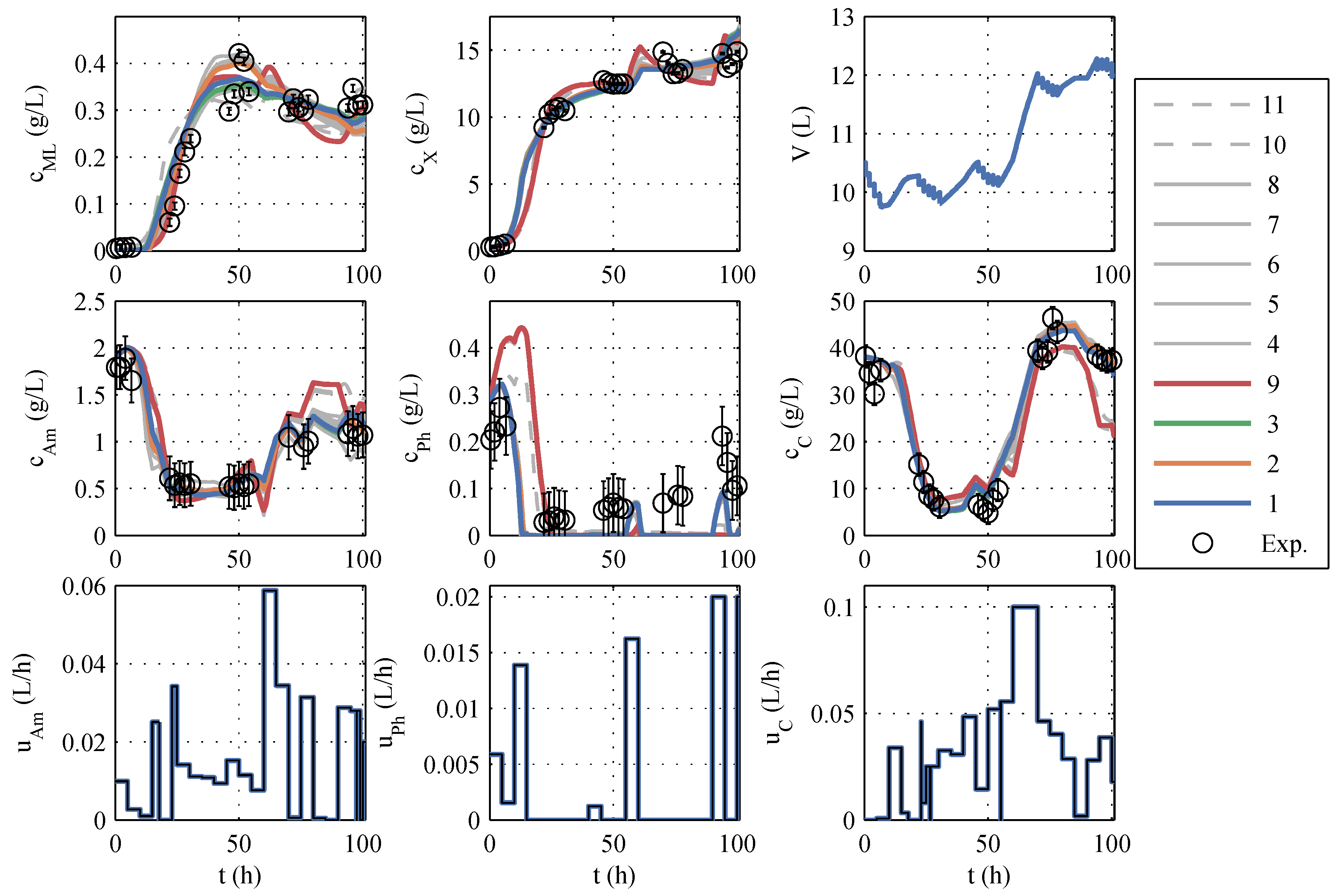
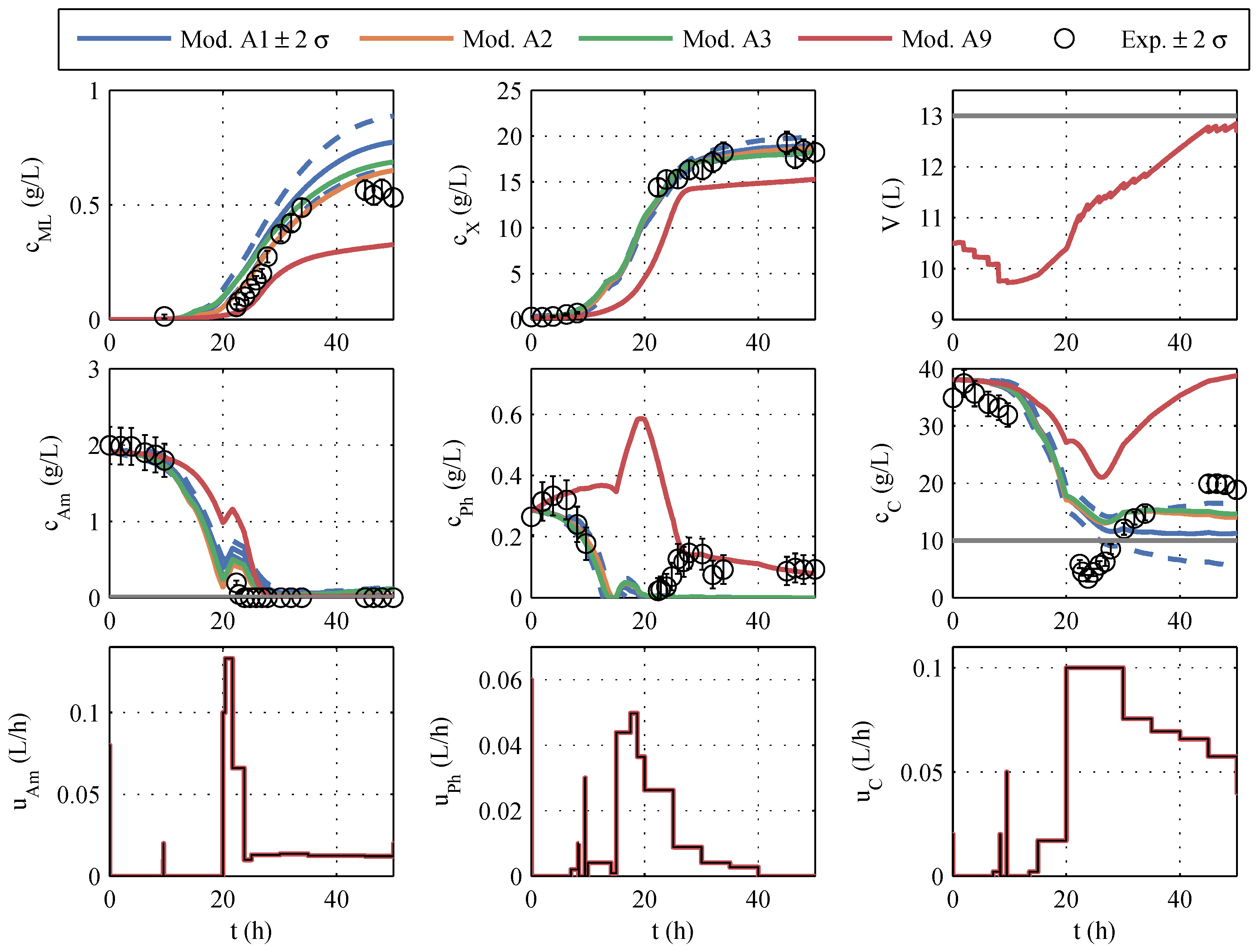
A typical identification experiment is given in Figure 1. Because phosphate storage in P.p. is also mentioned in the literature [39], the best model with a phosphate storage (No. 9) is also taken into account in further planning to cover structural uncertainties, even though Akaike ruled it out. The models to be further used are highlighted in color (red, green, orange, and blue) in Figure 1 and termed model family A (in

Table A1. Parameter values of model family A.

	Parameter	Value Mod. 1	Value Mod. 2	Value Mod. 3	Value Mod. 9	Unit
$r_{\mathrm{Xa}}$	${\mu }_{\mathrm{Xam}}$	0.0130	0.0406	0.0472	1.3274	1/h
	$K_{\mathrm{XaAm}}$	0.0542	0.0359	0.0475		g/L
	$K_{\mathrm{XaPh}}$	0.0099	0.0139	0.0158		g/L
	$K_{\mathrm{XaC}}$	0.00029	0.00023	0.00021	0.0001
	$K_{\mathrm{XaPhSt}}$				0.0002	g/L
$r_{\mathrm{zXa}}$	${\mu }_{\mathrm{dXam}}$	0.0561	0.0485	0.0497	0.0013	1/h
$r_{\mathrm{AmSt}}$	${\mu }_{\mathrm{AmStm}}$	0.0554	0.0342	0.0370		1/h
	$K_{\mathrm{AmStAm}}$	0.3815	0.2844	0.3614		g/L
	$K_{\mathrm{AmStPh}}$	3.2159	0.6581	0.0300		g/L
	$K_{\mathrm{AmStC}}$		0.0001			g/L
$r_{\mathrm{zAmSt}}$	${\mu }_{\mathrm{zAmStm}}$	0.2489	0.1467	2.2940		1/h
	$K_{\mathrm{zAmStAm}}$		0.0060			g/L
	$K_{\mathrm{zAmStPh}}$	16.6722	0.7386	31.0420		g/L
	$K_{\mathrm{zAmStC}}$		0.1443			g/L
$r_{\mathrm{CSt}}$	${\mu }_{\mathrm{CStm}}$	0.1608	0.1352	0.1185	0.1608	1/h
	$K_{\mathrm{CStC}}$	0.0001	0.0001	0.0001	0.0001	g/L
	$K_{\mathrm{CStAm}}$	0.0386	0.0257	0.0309	0.0386	g/L
	$K_{\mathrm{CStPh}}$	0.2572	0.3142	0.2797	0.2572	g/L
$r_{\mathrm{zCSt}}$	${\mu }_{\mathrm{zCStm}}$	0	0.0022	0	0	1/h
	$K_{\mathrm{zCStAm}}$	0.1003		0.1003	0.1003	g/L
	$K_{\mathrm{zCStPh}}$			0.1001		g/L
	$K_{\mathrm{zCStC}}$	0.0095		0.0097	0.0095	g/L
$r_{\mathrm{PhSt}}$	${\mu }_{\mathrm{PhStm}}$				0.2880
	$K_{\mathrm{PhStPh}}$				16.098
$r_{\mathrm{zPhSt}}$	${\mu }_{\mathrm{zCStm}}$				0.0862
$r_{\mathrm{Ml}}$	${\mu }_{\mathrm{Mlm}}$	0.0141	0.0173	0.0079	0.0068	1/h
	$K_{\mathrm{MlAm}}$	9.999	100	33.825	2.607	g/L
	$K_{\mathrm{MlPh}}$	0.0244	0.0152	0.0439	0.3427	g/L
	$K_{\mathrm{MlC}}$	20.902	8.919	39.521	100.0	g/L
$r_{\mathrm{zMl}}$	${\mu }_{\mathrm{zMlm}}$	0.0087	0.0116	0.0100	0.1668	1/h
$r_{\mathrm{M}}$	$Y_{\mathrm{M}}$	0.0488	0.0436	0.0423	0.0810	1/h
	$K_{\mathrm{M}}$	0.01	0.01	0.01	0.01	g/L
	$Y_{\mathrm{Xa}}$	31.402	9.133	8.233	5.578	g/g
	$Y_{\mathrm{PhXa}}$	3.6319	0.9241	0.7598	0.2646	g/g
	$Y_{\mathrm{CXa}}$	0.3083	3.1094	0.4393	13.7042	g/g
	$Y_{\mathrm{CCSt}}$	4.831	4.515	5.015		g/g

), and the remaining seven models are colored gray. The differences between the models are similarly large as the differences between the model and measured values. The AIC_c values also support this impression because no single model has a particularly high model probability. In other identification experiments (which are not shown here) the macrolactin simulation performed better. Model 9 was chosen as the best representative of its model structure, containing only a phosphate storage instead of ammonium and glucose storage. It is included in further process planning by manually assignind a model probability of 5%. It has to be noted that the decision to include model 9 was made before the extended model family B was developed. It turned out later that the phosphate storage approach is superior as will be discussed in the next subsection.

Overall, a purely visual differentiation and selection of the “best” model is difficult, and a model-based optimization based on only one seemingly “best”, nominal model would be at least questionable. For this reason, all good models als well as the best model with phosphate storage will be used, as shown below.

3.2. Extended Model (B)

The model family A was constructed fully automatically [40] and was used in the early modeling stage for robust planning; see Section 3.3.1 for the results. After performing the optimized experiment and installing process NIR spectroscopy as well as an online off-gas analysis, the new information was used to improve and extend the models towards a model family B.

There are some differences in the structure of model family A and model family B. The initial conditions such as the biomass concentration and the proportion of storage compartments within the cell in the inocolum are subject to disturbances. In model family A, the initial proportion of storage compartments was allowed to differ between experiments. The respective experiment-dependent parameters were found by optimization. The good adaptation that could be achieved in this way came at the expense of poor parameter identifiability. In the model family B, the parameters defining the proportion of storage compartments are set to a single global parameter for each component. The number of parameters that have to be determined by parameter identification is therefore drastically reduced and the identifiability is significantly improved.

Further changes from model family A to B concern biological phenomena. In family A, there is an “active biomass” Xa and there are storage compartments. Xa is degraded via a decay rate $r_{\mathrm{zXa}}$. The degraded biomass is not part of the measured biomass and is not converted back into substrates or any other usable form. This behaviour seems strange from a chemical and biological point of view. The source of this formulation could be automatic modelling based on the detection of phenomena.

After manual model checking, this behaviour is corrected in model family B. A state inactivated/deactivated biomass is added to the model, which consists of the cell-intern degraded active biomass.

$${\dot{m}}_{\mathrm{dX}}=r_{\mathrm{zXa}}·m_{Xa}$$

(18)

For the modeling of the carbon dioxide content in the exhaust gas, only active biomass and the maintenance metabolism were taken into account. The dynamic effects of mass transport and storage in the liquid were neglected. This resulted in the CO₂ mass flow entering the gas phase of

$$F_{\mathrm{in},{\mathrm{CO}}_2}=Y_{{\mathrm{CCO}}_2}\left(Y_{\mathrm{CXa}}{r}_{\mathrm{Xa}}(t)m_{\mathrm{XA}}(t)+Y_{\mathrm{M}}{r}_{\mathrm{M}}(t)m_{\mathrm{XM}}(t)\right);$$

(19)

The mass balance in the headspace can be written as follows:

$$\frac{\mathrm{d}}{\mathrm{d}t}{m}_{{\mathrm{CO}}_2}=F_{\mathrm{in},{\mathrm{CO}}_2}-600\mathrm{L}/\mathrm{h}·m_{{\mathrm{CO}}_2}/\left(22\mathrm{L}-V(t)\right);$$

(20)

It is assumed that ammonium is absorbed in the form of NH₃, so the H⁺ of the dissolved NH${}_3^{+}$ must be compensated by the corresponding amount of base added to keep the pH constant [71]. Further modeling approaches such as the production of organic acids in the context of an overflow metabolism are not considered. The differential equation for the mass of correction fluid base $m_{\mathrm{B}}$ results in the following:

$$\frac{\mathrm{d}}{\mathrm{d}t}{m}_{\mathrm{B}}=Y_{\mathrm{B}\mathrm{Am}}{r}_{\mathrm{Xa}}{m}_{\mathrm{Xa}}$$

(21)

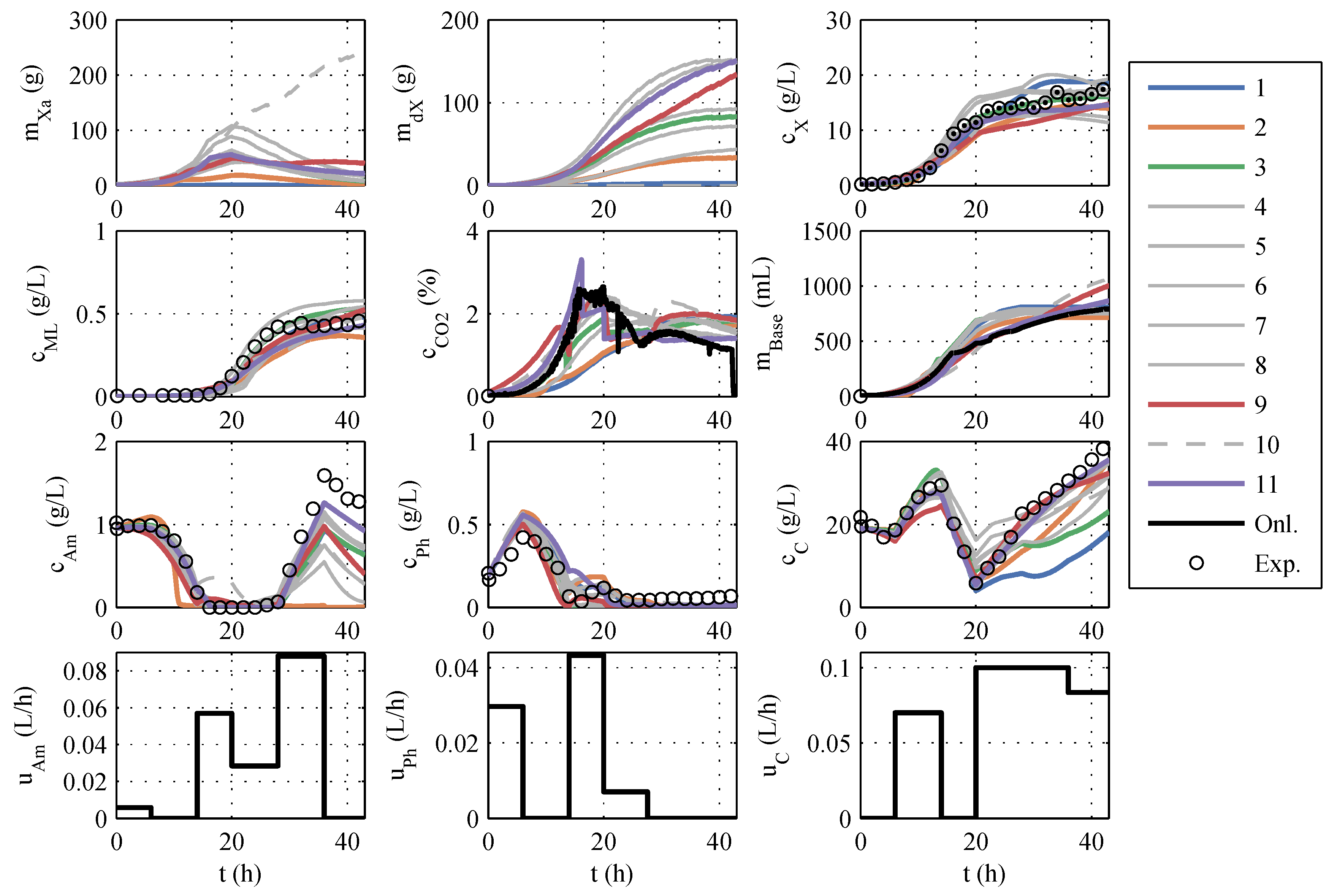
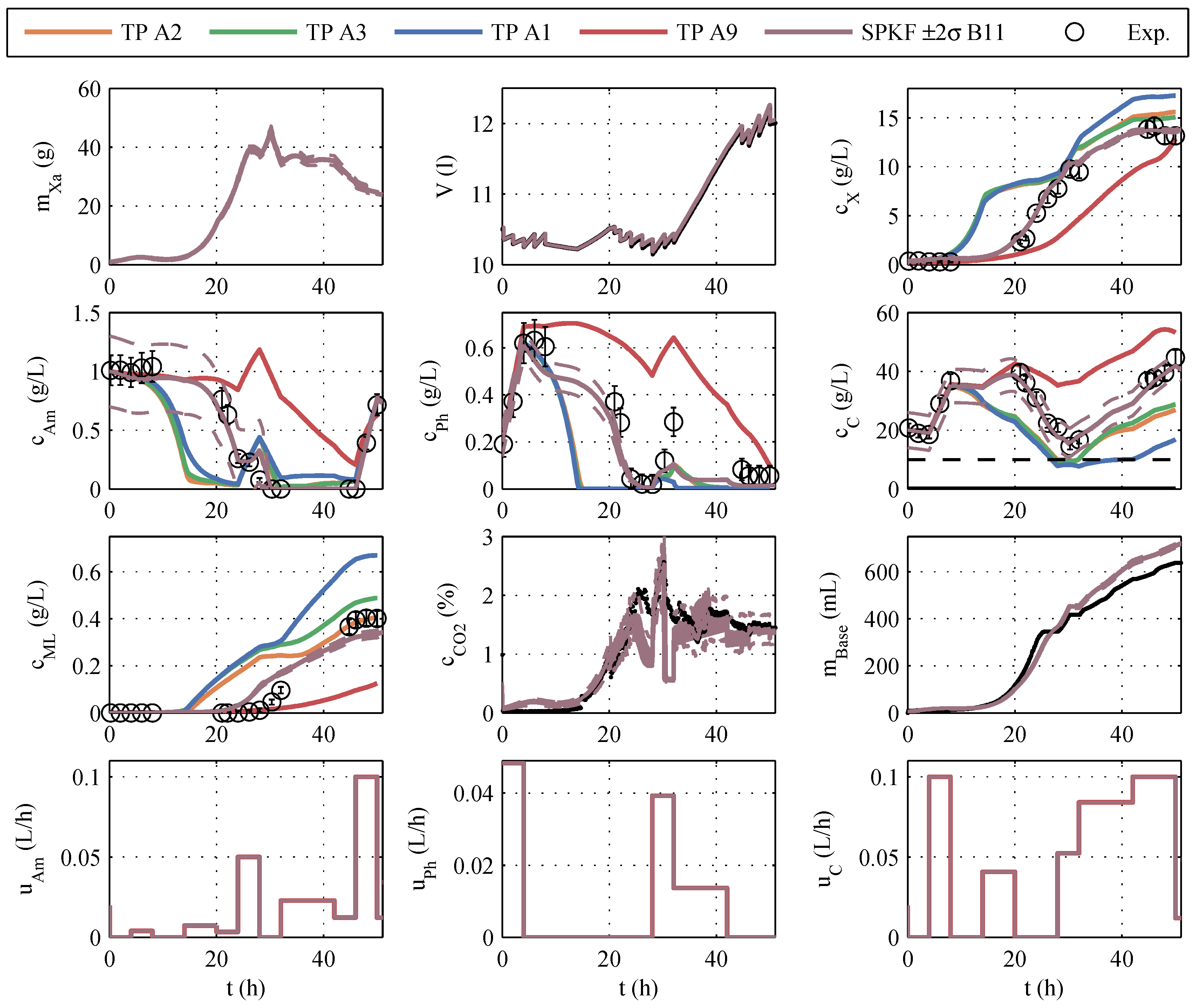
The models developed in this way are based directly on model family A, so the numbering of the models in Section 3.1 is retained. After implementing the model modifications, another parameter estimation was performed. A typical identification experiment is shown in Figure 2.

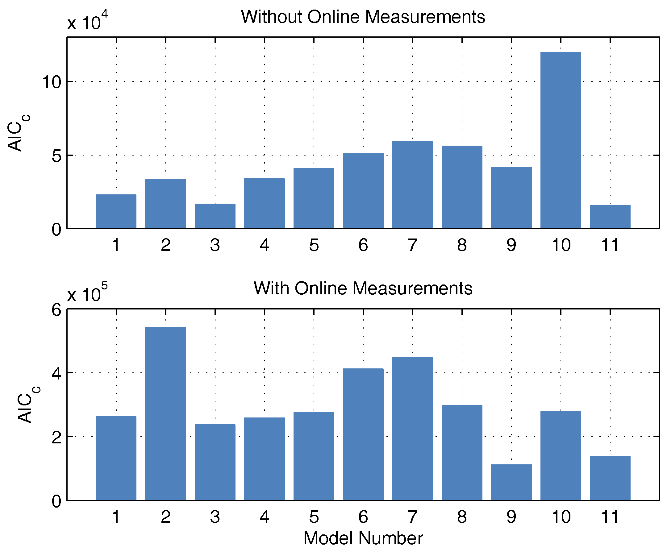
In contrast to the identification experiments of models A, the extended models show very large differences between the different models, especially in the description of CO₂, biomass, and glucose concentration. This could be because the additional measurement information is now available, while the number of parameters has increased only insignificantly. The AIC_c values and the corresponding probabilities are newly calculated. It is debatable whether the measurement data of CO₂ and base are to be considered in the calculation of the AIC_c. Both measured values have no influence on substrate consumption, biomass growth, and macrolactin production, and, therefore, are completely irrelevant for the process optimization. However, the correct description of the online measurements is relevant for the state estimation and should also be taken into account. Consequently, both approaches were pursued and are illustrated in Figure 3 in the form of AIC_c values. If the model probabilities are calculated without continuous measurement data, there is an Akaike probability of almost 100% for model 11. If online measurements are considered, model 11 also shows good performance because it scores second best with only a narrow distance to the best model but a large distance to the next-best model. Hence, model 11 is used for the online optimization and state estimation.

The differential equations for model 11, the parameter values, and the parameter standard deviations after the subset selection are given in the Appendix B.

NIR Spectroscopy

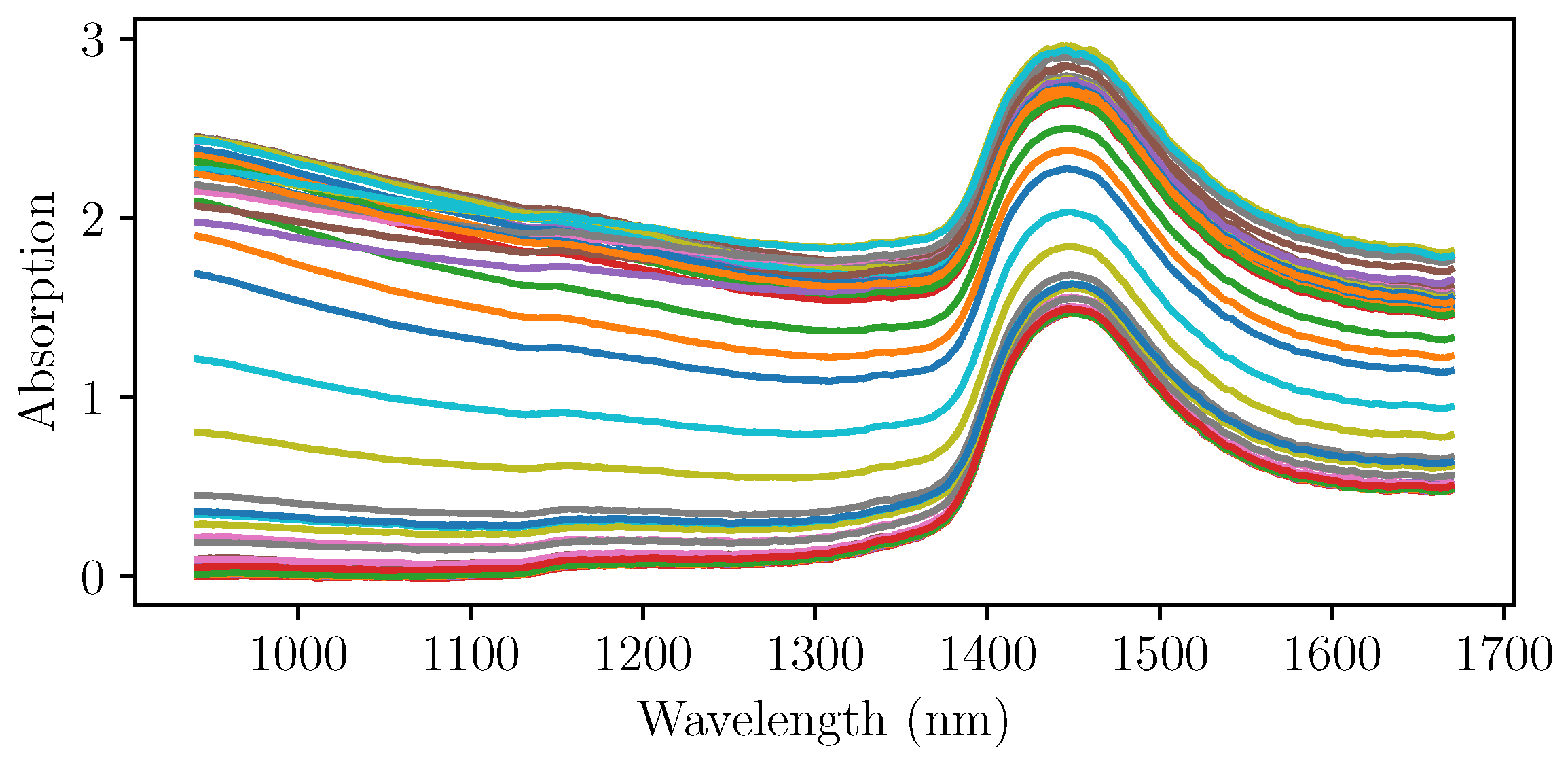
After the initial experiments, four more cultivations were run using NIR spectroscopy as an online measurement of the biomass concentration. The pretreated NIR spectra at the sampling times of the three cultivations that were used for the PLS regression are shown in Figure 4. It can be seen that the gradient with respect to the wavelength differs strongly, even at the same levels of absorption at wavelengths up to 1400 nm. A simple univariate intepretation that would focus on only one wavelenght would not yield the desired outcome.

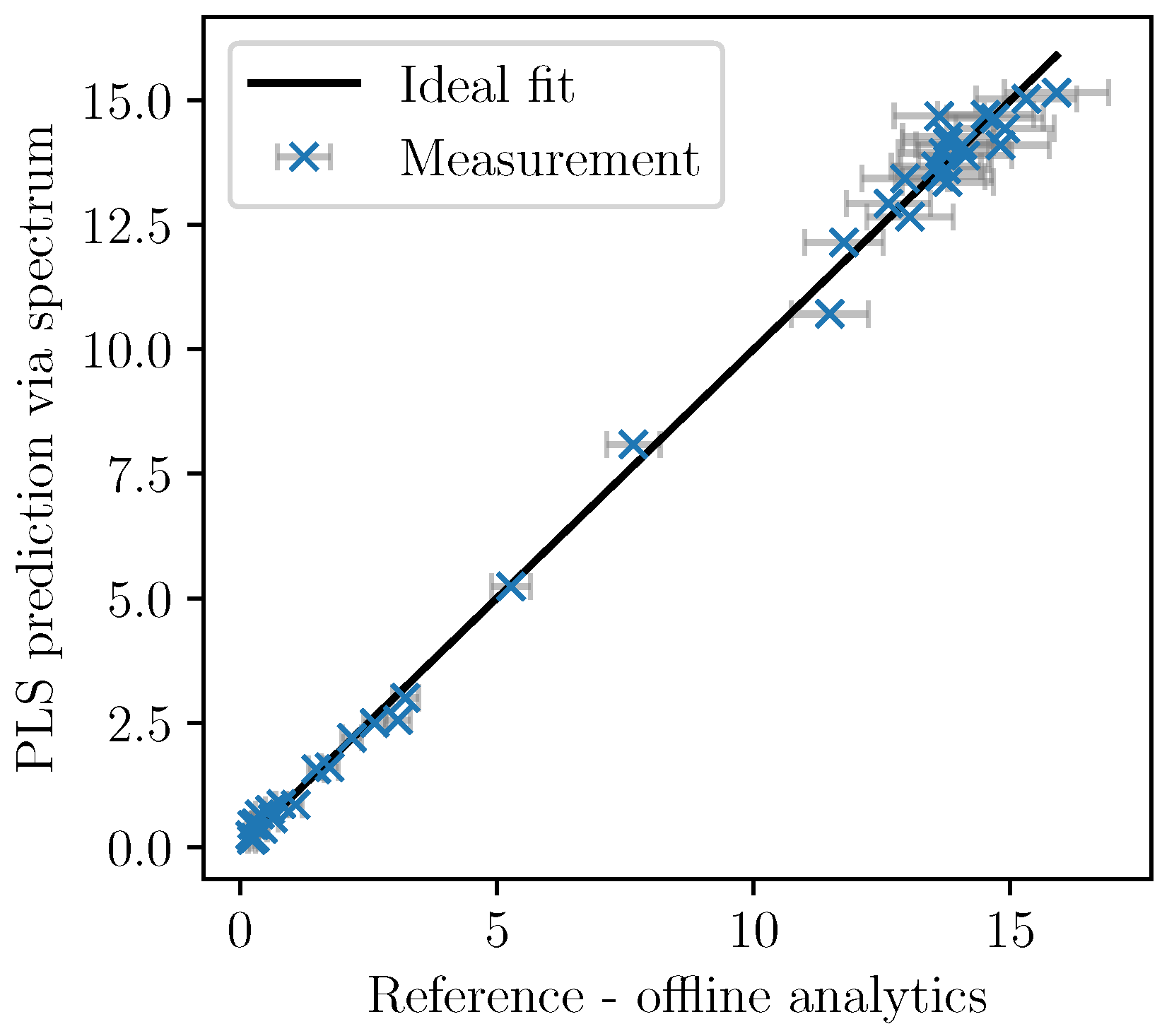
Based on the cross-validation, the number of factors was set to five. In Figure 5, the cross-validation of the PLSR predictions are plotted over the analytically measured reference values together with the ±2-$\sigma$ error bars of the measurements. The model shows good accordance as the deviation from the ideal fit could be explained by the measurement errors associated with the offline measurements.

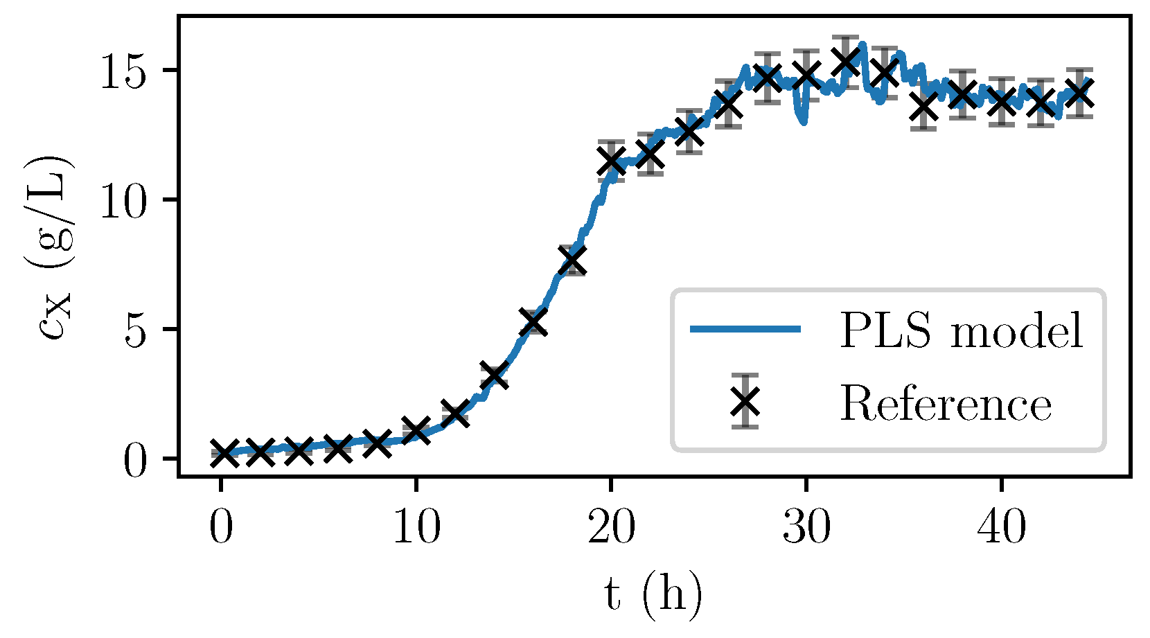
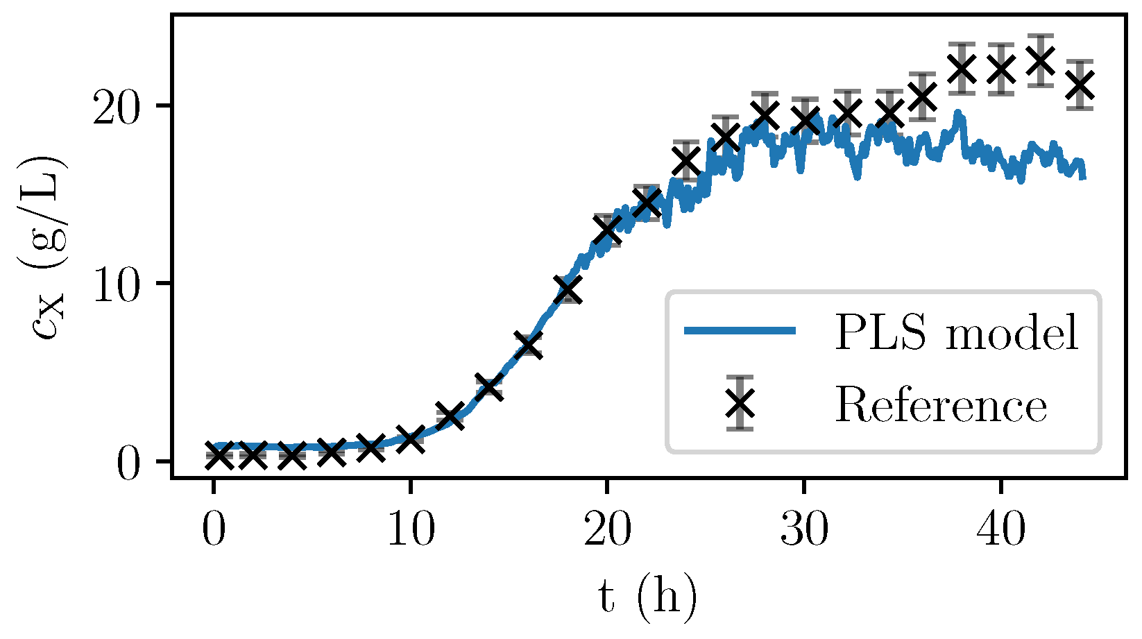
Only the spectra with corresponding offline-measurements were used for the calibration. Once identified, the PLS model can be used to calculate the PLS predictions of the biomass concentration based on the almost continuously recorded NIR spectra. In Figure 6, the values are given for a fermentation used for calibration. In Figure 7, the validation experiment not used for PLSR is depicted. In the validation cultivation, the biomass concentration surpasses the values that were reached in the calibration cultivations, as shown in Figure 5. Above 15 g/L of $c_{\mathrm{X}}$, large deviations occur. Furthermore, in the first eight hours, the prediction deviates significantly from the measurement data. All in all, PLS predictions are rather precise at medium biomass concentrations between 2 and 14 g/L. Therefore, NIR spectroscopy perfectly complements the CO₂ measurements that are more precise in the first part of the exponential growth phase at medium biomass concentrations between 0 and 2 g/L but that lack a good description of the limiting conditions.

No reliable PLS model was found for the substrates and macrolactin D.

3.3. Early-Stage Robust Optimization

The use case of the multi-model trajectory planning (MMTP) is the early process design while the model is still being improved. Only four cultivations were performed prior to the MMTP experiment; the following results are based only on the model family A.

3.3.1. Reference Nominal Process Optimization

Nominal trajectory planning serves as the reference method by choosing the best model of the model family, according to the AIC_c criterion and using it for offline optimization. To avoid a limitation by the limited oxygen input, a maximum biomass concentration of 20 g/L and a maximum biomass growth of 17 g/h was determined. To prevent the depletion of glucose, even in case of uncertainties, a lower limit of 10 g/L was set for the optimization.

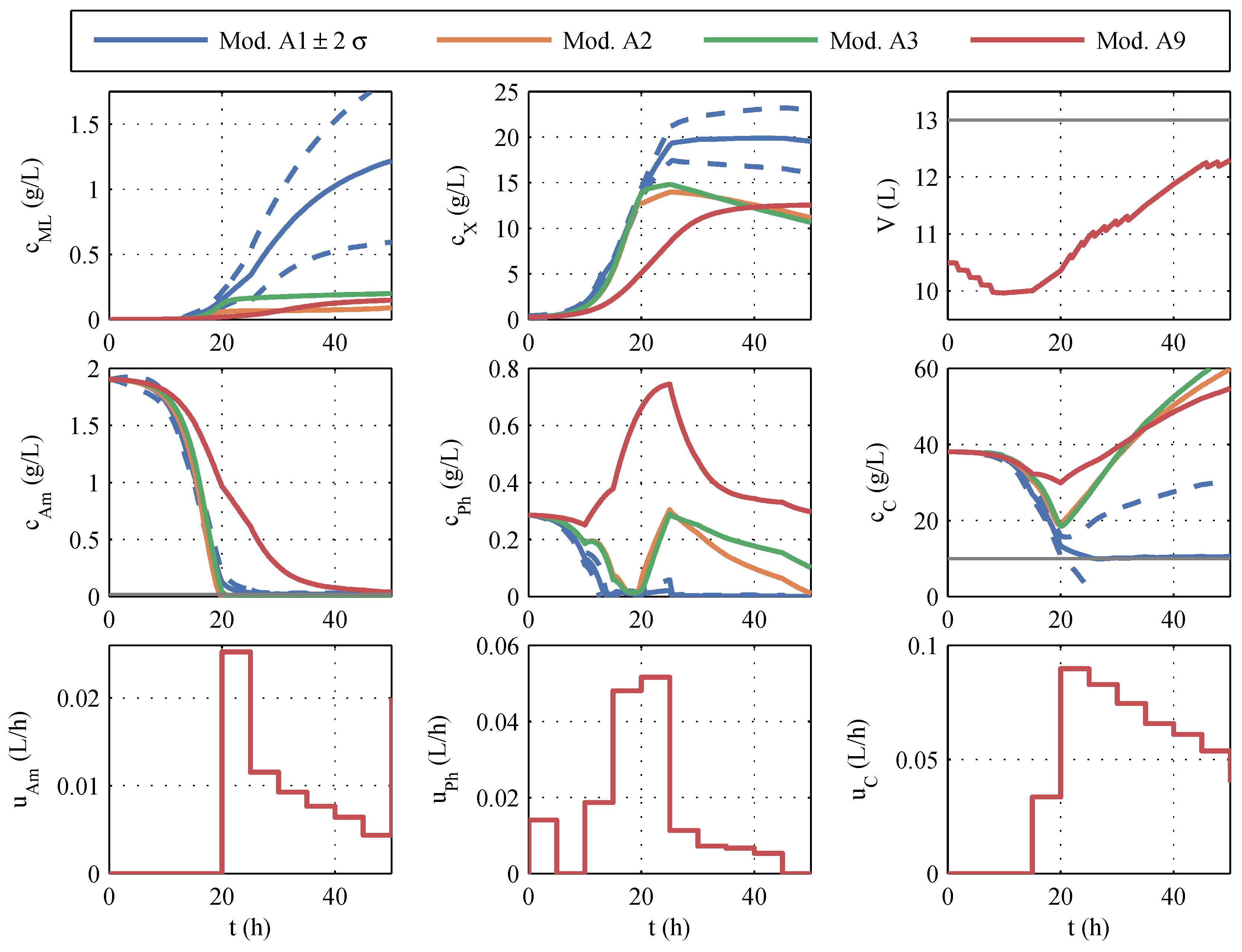
From the covariance matrix ${\mathbf{C}}_{\underline{\theta }\underline{\theta }}$, the predicted uncertainties of the measured variables during the fermentation process were determined via the state sensitivities. The volume, the concentrations of biomass, macrolactin, ammonium, phosphate, and glucose, as well as the control profiles of the optimal trajectory for model 1 and the $\pm 2$-$\sigma$ ranges of uncertainty, are shown in blue in Figure 8. In comparison, the curves of models 2, 3, and 9 are given, which occur if the manipulated variables optimized with model 1 were used for the simulation. Model 11 was not considered in this early phase, per Section 3.1.

In contrast to the parameter identification of model family A, the course of the various models differs considerably, shown in Figure 8. It is particularly noticeable in macrolactin production. The simulated macrolactin concentration with models 2, 3, and 9 is extremely low, whereas the quantity of 1.2 g/L computed with model 1 is significantly higher than the quantities achieved in the identification tests. Furthermore, it is noticeable that the simulation of the three models after 20 h fermentation time is far outside the ±2-$\sigma$ range of model 1 for almost all the measured variables. The range within $\pm 2$ standard deviations $\sigma$ comprises about 95% of the possible results. If one had relied solely on model 1, one would assume that macrolactin concentrations of less than 0.5 g/L occur only in 2.5% of the cases. However, all other models predict values below 0.2 g/L. These low macrolactin concentrations would be extremely unlikely according to model 1. However, according to the AIC_c, models 1, 2, and 3 were almost equally likely based on the set of the four first identification experiments. Therefore, it is evident that the parametric uncertainty of model 1 does not cover the uncertainty of the model choice.

3.3.2. Robust Planning and Experimental Validation

To address the problems outlined above, a subset of four models selected via the AIC_c criterion was used in robust planning (multi-model trajectory planning: MMTP) with Equation (13). For model 9, a probability of 5% was defined, and the other weights were based on their Akaike probability and adjusted accordingly. The simulated courses of substrate, biomass, and macrolactin concentrations are shown together with the experimental results in Figure 9.

For a comparison with the nominal planning, only simulations are available. The most important parameter here is the product quantity achieved. To compare the MMTP (using models 1, 2, 3, and 9) and nominal planning (using model 1), the respective optimal feeding profile is used for simulations with the models (1, 2, 3, and 9). The resulting macrolactin masses are given in

Table 3. Simulated makrolactin quantity at the end of fermentation; comparison of nominal and robust planning.

	Model No.
${\mathit{m}}_{\mathbf{ML}}({\mathit{t}}_{\mathbf{end}})$ in g	1	2	3	9	min	Weighted Mean
Nom. TP	15.0	1.1	2.5	1.8	1.1	6.6
MMTP	9.8	8.3	8.7	4.2	4.2	8.7

. For each case, the minimal and the mean macrolactin mass are determined and compared. Model 2 would yield only 1.1 g using the nominal optimization approach, whereas the smallest amount of macrolactin in the MMTP case is 281% higher. Similarly, the model-weighted mean is 33% higher for the MMTP case compared with the profiles obtained via nominal optimization. In the experimental realization, 6.8 g macrolactin were produced, which is less than the predicted average by the MMTP but still significantly more than the maximum 4.3 g achieved in the identification experiments. Furthermore, the effects of the parameter uncertainties on the fermentation were reduced without being explicitly taken into account. The computing time of the MMTP with an Intel i7 (3.07 GHz) of 72 min is only slightly more than twice as long as with the nominal planning, which requires 32 min.

3.4. Online Optimization

The multi-model approach can be omitted once a final model can be deducted and its parameters identified, which is the case here after four additional cultivations using online measurements of CO₂, consumed base, and NIR spectroscopy. From the extended and modified model family B, model 11 is found to be satisfactorily predictive on its own. However, besides the model uncertainty, there are other sources of deviations; for example, the initial biomass in the inoculum. Whereas offline robust optimization can only account for general deviations and leads to a very conservative design, online optimization can deal with the measured or estimated disturbances in the process hence leading to better results.

3.4.1. State Estimation

Only minimal tuning of the SPKF was necessary. The measurement uncertainty of the online measurements is not kept at the values that were determined experimentally. For the state estimation, the relative part a of Equation (2) is increased to take into account the deviation between the model value and measured value. The standard deviations of the corresponding measurements are given in

Table 4. Modified coefficients of Equation (2) for use in the state estimation.

	b in ${\%}_{{\mathbf{CO}}_2}$	b in mL	b in g/L
	CO2	Base	X NIR
a in %	7.5	7.5	5
b	0.1	3	0.5

. The measured value-dependent calculation of ${\sigma }_{\underline{y}}$ is particularly appropriate here because the CO₂ concentration and the base consumption at low values, i.e., in the exponential growth phase, are a very good indicator of growth, while the model uncertainty is much more pronounced at higher concentrations. The absolute measurement uncertainty of the CO₂ concentration was reduced to 0.1 ${\%}_{{\mathrm{CO}}_2}$ to take better advantage of this effect. For the NIR spectroscopy, the opposite is the case. High uncertainty was assumed at low biomass levels, while the relative error is smaller compared with the ${\%}_{{\mathrm{CO}}_2}$ and base.

No correlation between the measured values was assumed, R was hence a diagonal matrix with the corresponding variances. For the uncertainties of the initial values, a heuristic approach [67] yielded a relative deviation of ${\sigma }_{{\underline{\widehat{x}}}_0}=40\%$ for the biomass components and a value of ${\sigma }_{{\underline{\widehat{x}}}_0}=15\%$ for the remaining states. For the creation of sigma points, the parameter covariance matrix ${\mathbf{C}}_{\underline{\theta }\underline{\theta }}$ was used after the subset selection described above instead of Q. The corresponding standard deviations of the parameters are given in

Table A2. Parameter values of model B 11 with parameter standard deviation after subset selection.

Name	$\mathit{\theta }$	$\mathit{\sigma }$	$\mathit{\sigma }/\mathit{\theta }$	Name	$\mathit{\theta }$	$\mathit{\sigma }$	$\mathit{\sigma }/\mathit{\theta }$
${\mu }_{\mathrm{dXam}}$	0.14	0.0015	1.1%	$K_{\mathrm{XaAm}}$	0.0001	0.0002	184.1%
${\mu }_{\mathrm{MIm}}$	0.010	0.00030	3.1%	$K_{\mathrm{XaC}}$	0.0003	0.0001	33.6%
${\mu }_{\mathrm{PhStm}}$	0.043	0.00039	0.9%	$K_{\mathrm{XaPh}}$	0.0343	0.0005	1.6%
${\mu }_{\mathrm{Xam}}$	0.079	0.0004	0.5%	$K_{\mathrm{zPhStC}}$	0.0001	0.00017	166.0%
${\mu }_{\mathrm{zMlm}}$	0	-	-	$K_{\mathrm{M}}$	0.01	-	-
${\mu }_{\mathrm{zPhStm}}$	0.0116	0.00017	1.5%	$Y_{\mathrm{BAm}}$	0.024	0.00001	0.1%
$g_{0,\mathrm{PhSt}}$	0.75	0.007	0.9%	$Y_{\mathrm{M}}$	0.09	0.00054	0.6%
$K_{\mathrm{MIC}}$	100	9.77	9.8%	$Y_{{\mathrm{CCO}}_2}$	0.65	0.003	0.5%
$K_{\mathrm{MIPh}}$	0.084	0.007	8.1%	$Y_{\mathrm{PhXa}}$	0	-	-
$K_{\mathrm{MlAm}}$	5.66	0.36	6.4%	$Y_{\mathrm{Xa}}$	5.53	0.019	0.3%
$K_{\mathrm{PhSt}}$	0.077	0.0014	1.8%	$Y_{\mathrm{CXa}}$	14.58	0.044	0.3%

.

$${\mathbf{P}}_{xx,0}^{-}=\mathrm{diag}({({\sigma }_{{\underline{\widehat{x}}}_0}·{\underline{\widehat{x}}}_0^{-}+0.001)}^2)$$

(22)

The SPKF was tested with a cultivation, where the effects of large deviations in the inoculation biomass could be observed. Here, temperature fluctuations in the preculture phase led to a change in the inoculation biomass. The planned course of the offline robust process planning (MMTP) with model family A is given together with the experimental results in Figure 10. For illustration, the SPKF based on the new model B 11 was used to estimate and plot the states. The SPKF combines the complementary online measurements in an optimal way to determine the nonmeasurable states. A more detailed analysis is given in [8].

Observability

In all models, the rank of the observation matrix is lower than the respective system order, i.e., the number of estimated states. The differential equations obtained from mass balances, as shown in Appendix B, make it clear that the macrolactin quantity in the cultivation has no effect on the other states. Therefore, it is not possible to infer the macrolactin concentration indirectly via measurements. If one removes the mass of macrolactin from the system description and calculates the observability matrix again, its rank corresponds to the system order of the respective model at any time. Thus, all states save for the macrolactin mass are observable. However, it is not ensured that macrolactin converges with the actual value, but Figure 10 shows that the prediction nevertheless shows acceptable agreement with the offline measured values.

3.4.2. Experimental Application of Online Optimization

A final cultivation was performed to show the applicability of real-time optimization (RTO) with an SPKF state estimation. Every 0.1 h, a measurement update with the current online measurements was performed. Subsequently, the RTO was performed based on the newly estimated state. The constraints of the concentrations applied formerly to the MMTP were slightly adjusted. For the RTO, the upper biomass limit was removed, and the biomass growth limit was raised to 25 g/h because a better model quality allowed for a more precise estimation of growth and, therefore, fewer safety buffers were needed. The limitation of the glucose concentration to 10 g/L and the volume to 13 L were maintained.

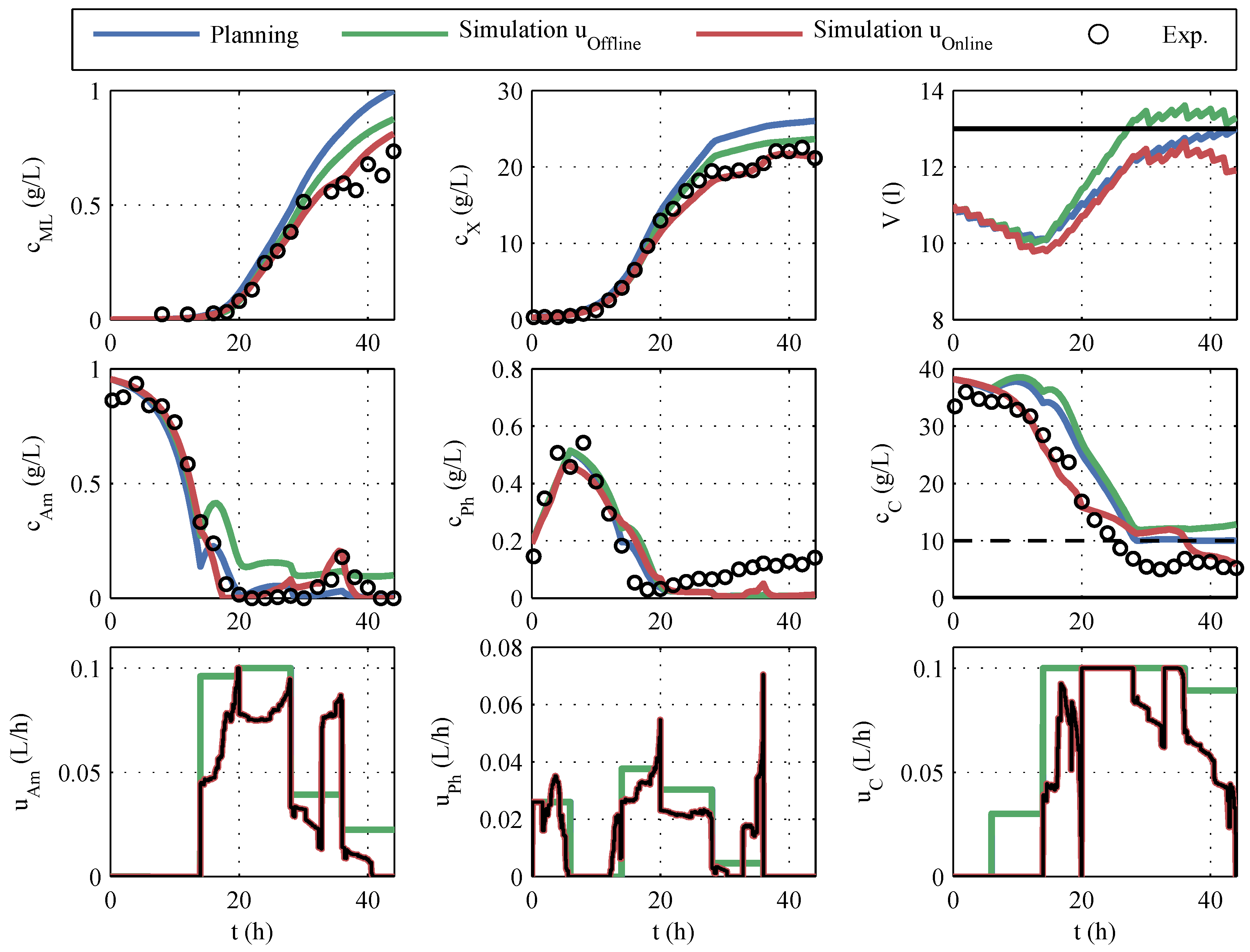
The experimental results of the online optimization are given in Figure 11. Additionally, different simulations are plotted. The result of the offline optimization is marked with planning in blue. In the initial offline optimization, the volumes of the correction fluids (acid, base, antifoam agent) were unknown and, therefore, not taken into account. The simulation $u_{\mathrm{Offline}}$ in green is obtained by using the offline optimized control variables together with the actually consumed correction fluids and the known sampling volumes for the simulation. The simulation $u_{\mathrm{Online}}$ in red corresponds to simulation $u_{\mathrm{Offline}}$, but the online-optimized control variables are used in the simulation.

The planning shows the highest predicted macrolactin concentration, but if this planning was to be carried out, the disregard of the correction fluids would result in a lower macrolactin concentration and an unacceptable violation of the volume constraint. The online optimization processes the SPKF’s current estimate of volume and, therefore, complies with the volume constraint but at a 7% lower predicted macrolactin concentration. If one compares the manipulated variable profiles in Figure 11 with the offline planning, it is noticeable that considerably less feeding volume was added. In

Table 5. Feeding volumes of offline and online planning for validation experiment.

Feeding Volume (L)	Offline TP	Online TP	Saving
Am	1.9	1.4	23%
Ph	0.7	0.6	9%
C	3.2	2.3	28%

, the impressive savings of the feeding quantities (28% for glucose) are summarized.

The comparison of hypothetical, simulated macrolactin quantities is only of limited significance. However, if one compares the macrolactin concentrations achieved, the RTO with 0.73 g/L eclipses the maximum concentrations of the offline robust process optimization (0.57 g/L). Because of the reduction of the fermentation duration from 50 h to 44 h, the improvement of the spacetime yield is even more pronounced.

4. Conclusions

The current experimental study showed the high performance of model-based approaches for process improvement. Based on a family of automatically built models (A), robust offline optimization led to increased macrolactin yield while ensuring that the constraints would be met by all the models. The use of nominal optimization based only on the best model would have underestimated the uncertainty of the model selection. Experimental validation confirmed the higher product yield that was achieved via robust process optimization even after only four cultivations. The performed experiments showed great discriminatory potential, leading to the selection of one superior model (B). The relatively simple model with only nine states in total permits good interpretability of the results and a low numerical burden for identification, as well as state estimation and optimization. However, even if the model uncertainty was greatly reduced, the influence of the deviations in the inoculum still had a large impact on the fermentation and its productivity. It has been shown how a SPKF can successfully estimate the course of the cultivation in real time based on the measurements of base consumption for pH control and CO₂ concentration in the off-gas. The use of process NIR spectroscopy with PLS regression was incorporated in the SPKF and led to an even more robust estimation because of its complementary measurement information. The use of real-time product maximization was successfully tested for the production of macrolactin D by Paenibacillus polymyxa. Besides reducing the amount of glucose feed by 28% compared with the offline planning, the optimization led to the largest mass of macrolactin compared with all other performed cultivations in the same setting.

Further investigations have to evaluate how well RTO can compensate for disturbances such as feeding pump failure and temperature fluctuations because the focus of the current contribution was on the process of model development and fast deployment of model-based methods in the process development.

References

1. Kawohl, M.; Heine, T.; King, R. Model based estimation and optimal control of fed-batch fermentation processes for the production of antibiotics. Chem. Eng. Process. Process Intensif. 2007, 46, 1223–1241. [Google Scholar] [CrossRef]
2. November, E.J.; Van Impe, J.F. The tuning of a model-based estimator for the specific growth rate of Candida utilis. Bioprocess Biosyst. Eng. 2002, 25, 1–12. [Google Scholar] [CrossRef] [PubMed]
3. Hitzmann, B.; Broxtermann, O.; Cha, Y.L.; Sobieh, O.; Stärk, E.; Scheper, T. The control of glucose concentration during yeast fed-batch cultivation using a fast measurement complemented by an extended Kalman filter. Bioprocess Eng. 2000, 23, 337–341. [Google Scholar] [CrossRef]
4. Dubach, A.; Märkl, H. Application of an extended Kalman filter method for monitoring high density cultivation of Escherichia coli. J. Ferment. Bioeng. 1992, 73, 396–402. [Google Scholar] [CrossRef]
5. Arndt, M.; Kleist, S.; Miksch, G.; Friehs, K.; Flaschel, E.; Trierweiler, J.; Hitzmann, B. A feedforward–feedback substrate controller based on a Kalman filter for a fed-batch cultivation of Escherichia coli producing phytase. Comput. Chem. Eng. 2005, 29, 1113–1120. [Google Scholar] [CrossRef]
6. Komives, C.; Parker, R.S. Bioreactor state estimation and control. Curr. Opin. Biotechnol. 2003, 14, 468–474. [Google Scholar] [CrossRef] [PubMed]
7. Dochain, D. State and parameter estimation in chemical and biochemical processes: A tutorial. J. Process Control 2003, 13, 801–818. [Google Scholar] [CrossRef]
8. Krämer, D.; King, R. A hybrid approach for bioprocess state estimation using NIR spectroscopy and a sigma-point Kalman filter. J. Process Control 2019, 82, 91–104. [Google Scholar] [CrossRef]
9. U.S. Department of Health and Human Services, Food and Drug Administration. Guidance for Industry: PAT—A Framework for Innovative Pharmaceutical Development, Manufacturing, and Quality Assurance; U.S. Department of Health and Human Services, Food and Drug Administration: Rockville, MD, USA, 2004.
10. Hinz, D.C. Process analytical technologies in the pharmaceutical industry: The FDA’s PAT initiative. Anal. Bioanal. Chem. 2006, 384, 1036–1042. [Google Scholar] [CrossRef]
11. Voss, J.P.; Mittelheuser, N.E.; Lemke, R.; Luttmann, R. Advanced monitoring and control of pharmaceutical production processes with Pichia pastoris by using Raman spectroscopy and multivariate calibration methods. Eng. Life Sci. 2017, 17, 1281–1294. [Google Scholar] [CrossRef] [Green Version]
12. Mehdizadeh, H.; Lauri, D.; Karry, K.M.; Moshgbar, M.; Procopio-Melino, R.; Drapeau, D. Generic Raman-based calibration models enabling real-time monitoring of cell culture bioreactors. Biotechnol. Prog. 2015, 31, 1004–1013. [Google Scholar] [CrossRef]
13. Li, M.; Ebel, B.; Chauchard, F.; Guédon, E.; Marc, A. Parallel comparison of in situ Raman and NIR spectroscopies to simultaneously measure multiple variables toward real-time monitoring of CHO cell bioreactor cultures. Biochem. Eng. J. 2018, 137, 205–213. [Google Scholar] [CrossRef]
14. Lopes, M.B.; Gonçalves, G.A.L.; Felício-Silva, D.; Prather, K.L.J.; Monteiro, G.A.; Prazeres, D.M.F.; Calado, C.R.C. In situ NIR spectroscopy monitoring of plasmid production processes: Effect of producing strain, medium composition and the cultivation strategy. J. Chem. Technol. Biotechnol. 2015, 90, 255–261. [Google Scholar] [CrossRef]
15. Scarff, M.; Arnold, S.A.; Harvey, L.M.; McNeil, B. Near infrared spectroscopy for bioprocess monitoring and control: Current status and future trends. Crit. Rev. Biotechnol. 2006, 26, 17–39. [Google Scholar] [CrossRef] [PubMed]
16. Landgrebe, D.; Haake, C.; Höpfner, T.; Beutel, S.; Hitzmann, B.; Scheper, T.; Rhiel, M.; Reardon, K.F. On-line infrared spectroscopy for bioprocess monitoring. Appl. Microbiol. Biotechnol. 2010, 88, 11–22. [Google Scholar] [CrossRef] [PubMed]
17. Lourenço, N.D.; Lopes, J.A.; Almeida, C.F.; Sarraguça, M.C.; Pinheiro, H.M. Bioreactor monitoring with spectroscopy and chemometrics: A review. Anal. Bioanal. Chem. 2012, 404, 1211–1237. [Google Scholar] [CrossRef] [PubMed]
18. Naysmith, M.R.; Douglas, P.L. Review of real time optimization in the chemical process industries. Dev. Chem. Eng. Miner. Process. 1995, 3, 67–87. [Google Scholar] [CrossRef]
19. Müller, D.; Dercks, B.; Nabati, E.; Blazek, M.; Eifert, T.; Schallenberg, J.; Piechottka, U.; Dadhe, K. Real-Time Optimization in the Chemical Processing Industry. Chem. Ing. Tech. 2017, 89, 1464–1470. [Google Scholar] [CrossRef]
20. Herwig, C. Hybrid Modelling and Multi-Parametric Control of Bioprocesses; MDPI AG: Basel, Switzerland, 2018. [Google Scholar] [CrossRef] [Green Version]
21. Dewasme, L.; Richelle, A.; Dehottay, P.; Georges, P.; Remy, M.; Bogaerts, P.; Vande Wouwer, A. Linear robust control of S. cerevisiae fed-batch cultures at different scales. Biochem. Eng. J. 2010, 53, 26–37. [Google Scholar] [CrossRef]
22. Craven, S.; Whelan, J.; Glennon, B. Glucose concentration control of a fed-batch mammalian cell bioprocess using a nonlinear model predictive controller. J. Process Control 2014, 24, 344–357. [Google Scholar] [CrossRef]
23. Cruz Bournazou, M.N.; Barz, T.; Nickel, D.B.; Lopez Cárdenas, D.C.; Glauche, F.; Knepper, A.; Neubauer, P. Online optimal experimental re-design in robotic parallel fed-batch cultivation facilities. Biotechnol. Bioeng. 2017, 114, 610–619. [Google Scholar] [CrossRef] [PubMed]
24. Barz, T.; Sommer, A.; Wilms, T.; Neubauer, P.; Cruz Bournazou, M.N. Adaptive optimal operation of a parallel robotic liquid handling station. IFAC-PapersOnLine 2018, 51, 765–770. [Google Scholar] [CrossRef]
25. Neddermeyer, F.; Marhold, V.; Menzel, C.; Krämer, D.; King, R. Modelling the production of soluble hydrogenase in Ralstonia eutropha by on-line optimal experimental design. IFAC-PapersOnLine 2016, 49, 627–632. [Google Scholar] [CrossRef]
26. Waldraff, W.; Biener, R.; Oswald, G.; Sippel, G.; King, R.; Gilles, E. Model-based control of bioprocesses-trajectory optimization and control. Biochem. Eng. 1993, 3, 171–173. [Google Scholar]
27. King, R. A structured mathematical model for a class of organisms: I. Development of a model for Streptomyces tendae and application of model-based control. J. Biotechnol. 1997, 52, 219–234. [Google Scholar] [CrossRef]
28. Waldraff, W.; King, R.; Gilles, E. Optimal feeding strategies by adaptive mesh selection for fed-batch bioprocesses. Bioprocess Eng. 1997, 17, 221–227. [Google Scholar] [CrossRef]
29. Levisauskas, D.; Galvanauskas, V.; Henrich, S.; Wilhelm, K.; Volk, N.; Lübbert, A. Model-based optimization of viral capsid protein production in fed-batch culture of recombinant Escherichia coli. Bioprocess Eng. 2003, 25, 255–262. [Google Scholar] [CrossRef]
30. Venkata Mohan, S.; Chandrasekhara Rao, N.; Krishna Prasad, K.; Murali Krishna, P.; Sreenivas Rao, R.; Sarma, P. Anaerobic treatment of complex chemical wastewater in a sequencing batch biofilm reactor: Process optimization and evaluation of factor interactions using the Taguchi dynamic DOE methodology. Biotechnol. Bioeng. 2005, 90, 732–745. [Google Scholar] [CrossRef]
31. Hüttel, S.; Müller, R. Methods to optimize myxobacterial fermentations using off-gas analysis. Microb. Cell Factories 2012, 11, 59. [Google Scholar] [CrossRef] [Green Version]
32. Herold, S.; King, R. Automatic identification of structured process models based on biological phenomena detected in (fed-)batch experiments. Bioprocess Biosyst. Eng. 2014, 37, 1289–1304. [Google Scholar] [CrossRef]
33. Herold, S.; Krämer, D.; Violet, N.; King, R. Rapid process synthesis supported by a unified modular software framework. Eng. Life Sci. 2017, 17, 1202–1214. [Google Scholar] [CrossRef] [Green Version]
34. Gustafson, K.; Roman, M.; Fenical, W. The macrolactins, a novel class of antiviral and cytotoxic macrolides from a deep-sea marine bacterium. J. Am. Chem. Soc. 1989, 111, 7519–7524. [Google Scholar] [CrossRef]
35. Yuen, G.Y.; Godoy, G.; Steadman, J.R.; Kerr, E.D.; Craig, M.L. Epiphytic colonization of dry edible bean by bacteria antagonistic to Sclerotinia sclerotiorum and potential for biological control of white mold disease. Biol. Control 1991, 1, 293–301. [Google Scholar] [CrossRef]
36. Schneider, K.; Chen, X.H.; Vater, J.; Franke, P.; Nicholson, G.; Borriss, R.; Süssmuth, R.D. Macrolactin is the polyketide biosynthesis product of the pks2 Cluster of Bacillus amyloliquefaciens FZB42. J. Nat. Prod. 2007, 70, 1417–1423. [Google Scholar] [CrossRef] [PubMed]
37. Okonkwo, C.; Ujor, V.; Mishra, P.; Ezeji, T. Process development for enhanced 2,3-butanediol production by paenibacillus polymyxa DSM 365. Fermentation 2017, 3, 18. [Google Scholar] [CrossRef] [Green Version]
38. Haughney, H.A.; Nauman, E.B. A bioenergetic model of a mixed production fermentation. Biotechnol. Bioeng. 1990, 36, 142–148. [Google Scholar] [CrossRef]
39. Violet, N.; Fischer, E.; Heine, T.; King, R. A software supported compartmental modeling approach for Paenibacillus polymyxa. IFAC Proc. Vol. 2010, 43, 377–382. [Google Scholar] [CrossRef]
40. Herold, S. Automatic Generation of Process Models for Fed-Batch Fermentations Based on the Detection of Biological Phenomena. Ph.D. Thesis, Technische Universität Berlin, Berlin, Germany, 2014. [Google Scholar]
41. Lantz, A.E.; Jørgensen, P.; Poulsen, E.; Lindemann, C.; Olsson, L. Determination of cell mass and polymyxin using multi-wavelength fluorescence. J. Biotechnol. 2006, 121, 544–554. [Google Scholar] [CrossRef]
42. Rhine, E.D.; Mulvaney, R.L.; Pratt, E.J.; Sims, G.K. Improving the berthelot reaction for determining ammonium in soil extracts and water. Soil Sci. Soc. Am. J. 1998, 62, 473. [Google Scholar] [CrossRef]
43. Walter, E.; Pronzato, L. Identification of Parametric Models from Experimental Data; Communications and Control Engineering; Springer: Berlin, Germany; New York, NY, USA; Masson: Paris, France, 1997. [Google Scholar]
44. Heine, T.; Kawohl, M.; King, R. Parameterschätzung für nichtlineare dynamische Modelle auf Basis stark verrauschter, statistisch unvollständig bestimmter Messdaten. Chem. Ing. Tech. 2003, 75, 543–550. [Google Scholar] [CrossRef]
45. Biegler, L.T. Nonlinear Programming: Concepts, Algorithms, and Applications to Chemical Processes; Society for Industrial and Applied Mathematics: Philadelphia, PA, USA, 2010. [Google Scholar]
46. Barz, T.; Kraus, R.; Zhu, L.; Wozny, G.; Arellano-Garcia, H. Generation of discrete first- and second-order sensitivities for single shooting. AIChE J. 2012, 58, 3110–3122. [Google Scholar] [CrossRef]
47. Violet, N. Software-unterstützte Erzeugung von mathematischen Modellen zur biotechnologischen Prozessführung. Ph.D. Thesis, Technische Universität Berlin, Berlin, Germany, 2016. [Google Scholar] [CrossRef]
48. Hurvich, C.M.; Simonoff, J.S.; Tsai, C. Smoothing parameter selection in nonparametric regression using an improved Akaike information criterion. J. R. Stat. Soc. Ser. B Stat. Methodol. 1998, 60, 271–293. [Google Scholar] [CrossRef]
49. Akaike, H. A new look at the statistical model identification. IEEE Trans. Autom. Control 1974, 19, 716–723. [Google Scholar] [CrossRef]
50. Olufsen, M.S.; Ottesen, J.T. A practical approach to parameter estimation applied to model predicting heart rate regulation. J. Math. Biol. 2013, 67, 39–68. [Google Scholar] [CrossRef] [PubMed] [Green Version]
51. Barz, T.; López Cárdenas, D.C.; Arellano-Garcia, H.; Wozny, G. Experimental evaluation of an approach to online redesign of experiments for parameter determination. AIChE J. 2013, 59, 1981–1995. [Google Scholar] [CrossRef]
52. Virtanen, P.; Gommers, R.; Oliphant Travis, E.; Haberland, M.; Reddy, T.; Cournapeau, D.; Burovski, E.; Peterson, P.; Weckesser, W.; Bright, J.; et al. SciPy 1.0–Fundamental algorithms for scientific computing in python. arXiv 2019, arXiv:1907.10121. [Google Scholar] [CrossRef] [Green Version]
53. Iglewicz, B.; Hoaglin, D.C. How to Detect and Handle Outliers; ASQ Press: Milwaukee, WI, USA, 1993. [Google Scholar]
54. Eilers, P.H.C. A perfect smoother. Anal. Chem. 2003, 75, 3631–3636. [Google Scholar] [CrossRef]
55. Mayerhöfer, T.G.; Mutschke, H.; Popp, J. Employing theories far beyond their limits—the case of the (Boguer-) Beer-Lambert Law. Chemphyschem A Eur. J. Chem. Phys. Phys. Chem. 2016, 17, 1948–1955. [Google Scholar] [CrossRef]
56. Wegelin, J.A. A Survey of Partial Least Squares (PLS) Methods, With Emphasis on the Two-Block Case; Technical Report 371; Department of Statistics, University of Washington: Seattle, DC, USA, 2000. [Google Scholar]
57. Savitzky, A.; Golay, M. Smoothing and differentiation of data by simplified least squares procedures. Anal. Chem. 1964, 36, 1627. [Google Scholar] [CrossRef]
58. Gill, P.E.; Murray, W.; Saunders, M.A. SNOPT: An SQP algorithm for large-scale constrained optimization. SIAM Rev. 2005, 47, 99–131. [Google Scholar] [CrossRef]
59. Gill, P.E.; Murray, W.; Saunders, M.A. User’s Guide for SNOPT Version 7: Software for Large-Scale Nonlinear Programming. 2006. Available online: https://web.stanford.edu/group/SOL/guides/sndoc7.pdf (accessed on 22 June 2020).
60. Johnson, M.E.; Moore, L.M.; Ylvisaker, D. Minimax and maximin distance designs. J. Stat. Plan. Inference 1990, 26, 131–148. [Google Scholar] [CrossRef]
61. Li, P.; Arellano-Garcia, H.; Wozny, G. Chance constrained programming approach to process optimization under uncertainty. Comput. Chem. Eng. 2008, 32, 25–45. [Google Scholar] [CrossRef]
62. Rossner, N.; Heine, T.; King, R. Quality-by-design using a gaussian mixture density approximation of biological uncertainties. IFAC Proc. Vol. 2010, 43, 7–12. [Google Scholar] [CrossRef] [Green Version]
63. Schwarm, A.T.; Nikolaou, M. Chance-constrained model predictive control. AIChE J. 1999, 45, 1743–1752. [Google Scholar] [CrossRef]
64. Srinivasan, B.; Bonvin, D.; Visser, E.; Palanki, S. Dynamic optimization of batch processes: II. Role of measurements in handling uncertainty. Comput. Chem. Eng. 2003, 27, 27–44. [Google Scholar] [CrossRef]
65. Srinivasan, B.; Palanki, S.; Bonvin, D. Dynamic optimization of batch processes: I. Characterization of the nominal solution. Comput. Chem. Eng. 2003, 27, 1–26. [Google Scholar] [CrossRef]
66. Van der Merwe, R.; Wan, E.A.; Julier, S.I. Sigma-point Kalman filters for nonlinear estimation and sensor-fusion: Applications to integrated navigation. In Proceedings of the AIAA Guidance, Navigation & Control Conference, Providence, RI, USA, 13–16 August 2004. [Google Scholar]
67. Schneider, R.; Georgakis, C. How to not make the extended kalman filter fail. Ind. Eng. Chem. Res. 2013, 52, 3354–3362. [Google Scholar] [CrossRef]
68. Gelb, A. Applied Optimal Estimation; M.I.T. Press: Cambridge, MA, USA, 1974. [Google Scholar]
69. Villaverde, A.F.; Barreiro, A.; Papachristodoulou, A. Structural identifiability of dynamic systems biology models. PLoS Comput. Biol. 2016, 12, e1005153. [Google Scholar] [CrossRef] [Green Version]
70. Villaverde, A.F.; Tsiantis, N.; Banga, J.R. Full observability and estimation of unknown inputs, states and parameters of nonlinear biological models. J. R. Soc. Interface 2019, 16, 20190043. [Google Scholar] [CrossRef] [Green Version]
71. Ludewig, U.; Neuhäuser, B.; Dynowski, M. Molecular mechanisms of ammonium transport and accumulation in plants. FEBS Lett. 2007, 581, 2301–2308. [Google Scholar] [CrossRef] [Green Version]
Figure 1. Identification experiment for model family A; the models used for further planning are highlighted in color. Concentrations of a substance i are given as c i , and u j denotes a feed stream.
Processes 08 00752 g001
Figure 2. Identification experiment for model family B; models used for planning are highlighted in color.
Processes 08 00752 g002
Figure 3. AICc values for the modified model family (B) with and without consideration of online measurement data.
Processes 08 00752 g003
Figure 4. Pretreated NIR spectra of different cultivations used for PLS regression.
Processes 08 00752 g004
Figure 5. Cross-validation prediction of biomass concentrations based on NIR spectra using PLS regression.
Processes 08 00752 g005
Figure 6. Online biomass concentration based on PLS model auto-validation.
Processes 08 00752 g006
Figure 7. Online biomass concentration based on PLS model external validation.
Processes 08 00752 g007
Figure 8. Comparison of the experiment planned with model 1 and simulation of it with models 2, 3, and 9.
Processes 08 00752 g008
Figure 9. Robust planning using models 1, 2, 3, and 9 with offline values of the experimental validation. Optimization constraints for the volume and glucose are depicted as gray lines.
Processes 08 00752 g009
Figure 10. SPKF using online data compared with the preceding planning and offline measurements for a cultivation with large deviations of the initial biomass, where TP A1, A2, A3, and A9 represent the simulated evolution with the respective model based on the offline robust planning (MMTP).
Processes 08 00752 g010
Figure 11. Comparison of the preceding offline planning with online optimization together with offline measurements.
Processes 08 00752 g011