Application of Combined Developments in Processes and Models to the Determination of Hot Metal Temperature in BOF Steelmaking

Abstract

Nowadays, the steel industry is seeking to reduce its carbon footprint without affecting productivity or profitability. This challenge needs to be supported by continuous improvements in equipment, methods, sensors and models. The present work exposes how the combined development of processes and models (CDPM) has been applied to the improvement of hot metal temperature determination. The synergies that arise when both sides of this research are simultaneously approached are evidenced. A workflow that takes into account the CDPM approach is proposed. First, a thermal model of the process is developed, making it possible to identify that hot metal temperature is a key lever for carbon footprint reduction. Then, three main alternatives for hot metal temperature determination are compared: infrared thermometry, time-series forecasting and machine learning prediction. Despite considering only few process variables, machine learning techniques succeed in extracting relevant information from process databases. An accuracy close to infrared thermometry is obtained, with a much higher applicability. This research shows that process-model alternatives are complementary when judiciously nested in the process computer routines. Combining measurement and modelling techniques, 100% applicability is achieved with an error reduction of 7 °C.

1. Introduction

Steel is a highly recyclable material. Consequently, the electric arc furnace (EAF), which produces steel mostly from scrap collected from recycling, is the most direct method of steelmaking. However, the increasing demand for steel cannot be met only by recycling, and new metallic iron must enter the global cycle, either through the direct reduction of iron ores or through integrated steelmaking. This prevailing route uses the blast furnace (BF) to produce iron from iron ore; in a second step, a basic oxygen furnace (BOF) converts this crude iron, with some scrap and other material additions, into steel.

Integrated steelmaking accounts for 70% of world steel production [1]. It uses large amounts of carbon as a reducing agent and generates CO₂. On the other hand, the EAF route is simpler, uses fewer natural resources, consumes less energy and generates fewer CO₂ emissions. This is the paradox and challenge of the steel industry. Steel is a material that fits perfectly into the circular economy, but the need to introduce new metallic iron into the global cycle causes a significant carbon footprint. Today, the steel industry is seeking to reduce its CO₂ emissions without affecting productivity or profitability [2]. This adaptation must not rely solely on breakthrough innovations; it must also be supported by the continuous improvements in equipment, methods, sensors and models [3,4].

Focusing on the BOF process, considerable modelling effort has been made, although it is unclear whether this has always been in the right direction. The potential benefits of complex models over other, simpler alternatives are seldom mentioned. For instance, descriptions have been published of several models for the prediction of the BOF endpoint [5,6], for which sensors have long existed for reliable endpoint determination [7]. By contrast, little attention has been paid to the modeling of the BF–BOF interface, despite its strong energy implications [8,9]. Some phenomenological thermal models have been described in the literature [10,11,12], although their real applicability and long-term sustainability were not reported. Only very recently has the search for improved hot metal temperature predictions been addressed [13,14,15]; using a systematic procedure, the present work compares the various alternatives for this purpose.

In a separate contribution [16], the authors will review the features and benefits of the combined development of processes and models (CDPM). Essentially, this approach is based on the characteristics highlighted by Alexander McLean in the early 2000s [3], and has gained the interest of the authors over the course of several projects for the optimization of energy processes [13,14,15,17]. The present work describes how these ideas have been successfully applied to the improvement of hot metal temperature determination using sensors and models. It will serve to illustrate the synergies that arise when both aspects are addressed simultaneously.

This research is focused on BOF process and the BF–BOF interface, as illustrated in Figure 1 [18,19]. BF produces liquid iron, called hot metal. The hot metal is pretreated and transferred to the BOF, where it is transformed into liquid steel. While the hot metal composition remains rather stable from the blast furnace to the steel mill, its temperature undergoes a variable drop, so its exact value is not known at the moment of the BOF load calculation. However, an estimation of the actual hot metal temperature (y in Figure 1) is required to calculate the relative quantities of hot metal, scrap and other raw materials to be included. Given that these materials account for a significant part of the cost of steel and the associated carbon footprint, accurate forecasting of the hot metal temperature becomes critical for the optimization of the BOF process [20].

The aim of this work is to illustrate how a CDPM approach can be reinvented based on previous existing ideas and adapted to this complex process, generating a working method for process improvement. It is then applied to identify which aspects of the BOF process have the greatest impact on the carbon footprint. Additionally, mitigation measures are addressed through the concurrent development of processes and models.

This article is organized as follows. Section 2 proposes a workflow that takes into account the CDPM approach, and then describes a thermal model of the BOF with which it is possible to identify the main actuators for carbon footprint reduction, before analyzing three key alternatives for hot metal temperature determination: (1) infrared thermometry measurement; (2) time-series forecasting; and (3) machine learning predictions. The results of these techniques are presented in Section 3 and discussed in Section 4, where relevant synergies between them are identified.

2. Materials and Methods

2.1. Proposed Workflow

As described, the joint development of processes and models appears to be a better approach than conducting isolated efforts. However, no information has yet been published on a possible workflow for applying these principles. In order to fill this gap, and for this particular research, the authors used and adapted CRISP-DM (Cross-Industry Standard Process for Data Mining). This methodology was conceived in the late 1990s in the framework of a European Union project [21]. Nowadays, it represents the most widely used workflow for data-mining modeling [22]. It is preferred over other methods because it emphasizes the understanding of business (i.e., the process) and data (the model), which is the central dichotomy of the CDPM approach.

As shown in Figure 2, the key steps of the original CRISP-DM were split in two: one line for process development and the other for model development. An additional previous step was added which considers several process-model alternatives. This latter step takes into account possible synergies between both approaches and avoids unnecessary overlapping between them. In addition, a final joint evaluation of the selected alternatives was added. This step provides a final image and identifies the best solution for implementation.

2.2. Process-Model Understanding

As indicated in Figure 2a, the first and possibly the most important step of the CRISP-DM workflow is an adequate understanding of the process under consideration. In the view and experience of the authors, process understanding must be supported by adequate process modeling. It is clear that the contribution of process experts is crucial in this stage, but this may be insufficient. Since process experts may not be fully aware of all the existing crossed effects and implications, collaboration with modeling experts is desirable in order to set up a valid model of the complete process. The model must be capable of simulating the behavior of the system at all possible operating points.

Already published models of the BOF process are often either too broad (site or regional scale [23,24,25]) or too narrow (individual effects [26,27]). In order to adequately describe the BOF converter, and to assess the relative importance of the involved variables, a complete mathematical description of the process was proposed [17]. Since such a model must adequately describe thermal aspects of the process in the complete operating domain, a model based on mass and energy balances was adopted. A macroscopic, law-driven model tends to generalize well [4], and can be successfully applied in different plants and under diverse production scenarios. The proposed approach is substantially different from the classical models used to control the BOF process. These well-established models rely heavily on the continuous statistical updating of their parameters. Consequently, they are very accurate for short-term forecasting, but they lose their reliability when applied to extended periods of time, or to different operating points or plants.

The BOF converter is a batch reactor; each batch is commonly referred to as a “heat”. As shown in Figure 1, the main input materials, i.e., hot metal and scrap, are loaded into the empty converter at the beginning of the process. Afterwards, different materials such as oxygen, argon and lime are added continuously or intermittently over a total time of about 15 min. A continuous off-gas flow is generated along the process. At the end of the process, the converter is emptied, yielding steel as the product and liquid slag as a byproduct.

The proposed thermal model takes into account mass and energy balances, as well as the enthalpy of the highly exothermic oxidation reactions occurring inside the converter. These three aspects are coupled. The mass balance can be expressed as:

$${\displaystyle \sum }_{i\in input}{m}_i{x}_i^j={\displaystyle \sum }_{i\in output}{m}_i{x}_i^j$$

(1)

where m_i is the mass of material i involved in the process as input, output or both, and $x_i^j$ is the mass fraction of species j in material i. The energy balance can be expressed as:

$$-\Delta H_r^M={\displaystyle \sum }_{i\in output}{m}_{i }\Delta h_{M-F}{}_i-{\displaystyle \sum }_{i\in input}{m}_i \Delta h_{M-I}{}_i+Q_{TL}$$

(2)

where $-\Delta h_{M-I}{}_i$ represents enthalpy variation, including the decomposition, heating and dissolution, of the input material i from initial to metallurgical conditions (1600 °C, 1 atm). The term $\Delta h_{M-F}{}_i$ is the enthalpy variation of output material i from the metallurgical to the final conditions. The reaction enthalpy under metallurgical conditions is represented by $\Delta H_r^M$ and the thermal losses by $Q_{TL}$. Equation (2) indicates that the enthalpy of exothermic reactions ($-\Delta H_r^{M }>0$) contributes to: (a) increasing the enthalpy of the input materials from initial to metallurgical conditions ($-\Delta h_{M-I}>0$); (b) increasing the enthalpy of products from metallurgical to final conditions ($\Delta h_{M-F}{}_i>0)$; and, finally, (c) thermal losses $(Q_{TL}>0)$.

The balances expressed in Equations (1) and (2) were applied to the eleven relevant species involved in the process: Fe, C, Si, Mn, P, CaO, MgO, SiO₂, O₂, Ar and N₂. Ten input materials were considered: hot metal, scrap, lime, dolomitic lime, iron ore, anthracite, FeSi, nitrogen, argon and oxygen. The three output phases are steel, slag and off-gas. Details of the resulting equation system were given in previous related works [17,28].

The stoichiometry of the oxides in the slag are known for SiO₂, MnO and P₂O₅; for iron, it is assumed that Fe²⁺/(Fe²⁺ + Fe³⁺) = 0.3. Additionally, the iron content of the slag is assumed to be $x_{slag}^{Fe}$ = 0.18, which is a common target in BOF steelmaking. The ratio for carbon oxidation in the vicinity of the bath, CO/(CO+CO₂), was taken as 0.9. Reaction and transformation enthalpies were obtained from the literature [19,29,30,31,32]; in case of discrepancies between sources, the one closest to actual industrial experience was used. Finally, thermal losses were taken to be 5% of the energy input, as suggested by Kudrin [29] and confirmed by plant data.

This thermal model allowed us to evaluate the material and energy flows of the BOF process under any operating conditions. The model was validated against real plant data and then applied to assess the impact of the process parameters on carbon emissions [17]. Indirect emissions were obtained from Ryman and Larsson [33]. It was found that hot metal temperature management is a primary actuation lever at the BF–BOF interface, as illustrated in Figure 3. Moreover, as depicted in Figure 4, reducing the absolute error in hot metal temperature forecasting by 10 °C contributed to a reduction of 5 kg of CO₂ per ton of liquid steel. A positive error in temperature is compensated for by the addition of anthracite. This will cause a net increase in total emissions of approximately 5 kg of CO₂ per ton of liquid steel. On the other hand, a negative error would require the addition of iron ore as a coolant. This addition does not appreciably increase emissions, but the excess hot metal is responsible for a similar increase in CO₂ emissions.

2.3. Process and Model Alternatives

In order to achieve a better forecast of the hot metal temperature at the steel mill, different methods can be envisaged. They can be grouped into four main axes:

• Direct measurement with thermocouples
• Indirect measurement with IR thermometer
• Prediction with stochastic models
• Prediction with machine learning models

The first and second alternatives pertain to process development, while the third and fourth correspond to model development.

2.4. Process Development

2.4.1. Direct Measurement

The hot metal temperature is required to calculate the BOF load [34]. At first glance, the easiest way to obtain this value is to use disposable thermocouples; this is a reliable measurement method, since the instrument has sufficient accuracy, and repeatability has been validated in steelmaking practice [35]. There are two possible moments for doing this:

• On the torpedoes, directly before starting pouring
• On the hot metal ladle, before completing the hot metal transfer

However, the direct measurement option presents some important drawbacks:

• Several automated measuring stations and additional labor would be required to measure on torpedoes, since several hot metal transfer points exist at each steel mill. If the measurement is to be made on hot metal ladles, at least two measuring stations would be necessary.
• Direct measurement implies delaying the execution of the BOF load model until the last possible moment. This requires that not only the preparation of the hot metal, but also the preparation of the associated scrap load be postponed. This has a very negative impact on the productivity of the steel mill.
• Despite the fact that thermocouples are accurate, the obtained temperature is not representative of the real conditions in which the hot metal will finally be loaded into the converter. To remedy this, several processes occurring after the thermocouple measurement would require additional modelling, e.g., the holding time in the torpedo, hot metal pouring from the torpedo to the ladle, the holding time in the ladle and the skimming of the hot metal ladle.

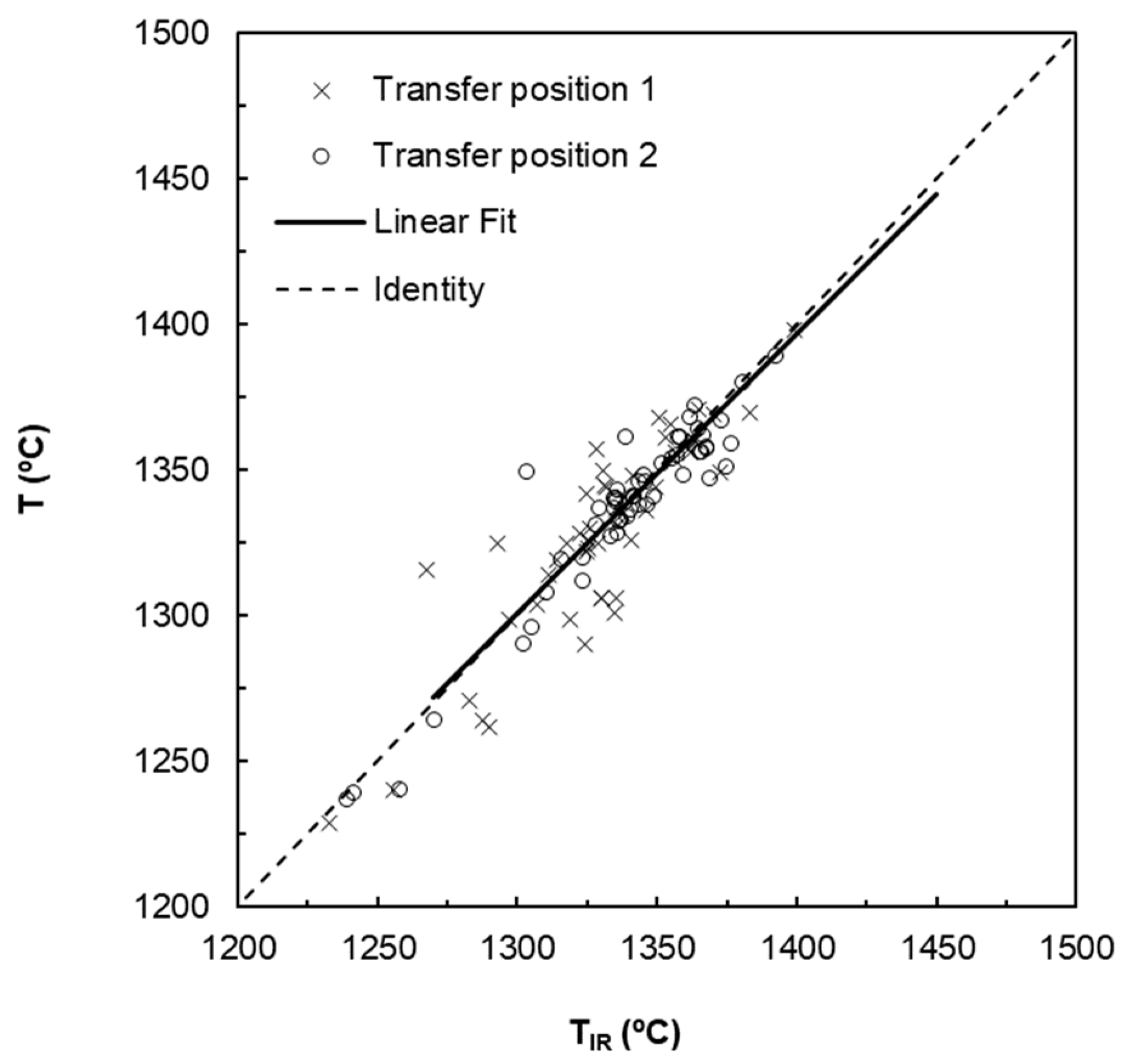
2.4.2. Indirect Measurement

A second possibility is indirect, contactless measurement with infrared (IR) thermometry on the hot metal stream during pouring. This would mitigate some of the aforementioned drawbacks, although new weak points may arise. The effect of drawbacks (1) and (2) would be partially reduced, since the measurement is carried out without altering the normal transfer process, albeit at the last minute. In contrast, the limitation (3) is maintained—or even increased—due to the uncertainties associated with the position of the hot metal stream and the presence of sparks, fumes and slag.

In previous research [14], a series of tests were carried out on 220 heats. The thermocouple results were compared with the IR measurements. Moreover, video sequences were simultaneously recorded in order to identify and understand the main causes of IR signal disturbance. The ratio of complete and successful IR measurements was rather low, i.e., approximately 60%. The main cause for this was the variability of the shape and the position of the stream. However, a good value of the mean absolute error, i.e., 11 °C, was obtained, after performing a linear regression adjustment, as indicated in Figure 5.

2.5. Model Development

The BF–BOF interface has a strong impact upon raw materials, energy and emissions. Consequently, the modeling of the thermal aspects has received much attention in recent decades, often focusing on individual subprocesses of the interface. There are few general models dedicated to predicting the evolution of the temperature between the blast furnace and the steel mill. This is not comparable to the attention paid to temperature evolution in downstream processes, from the BOF converter to the continuous casting [36].

Although some phenomenological models have been proposed in the past [10,11,12], such approaches are not suitable to control models under real plant conditions, since many relevant phenomena and variables are difficult to measure, or even to minimally characterize. For this reason, a data-driven approach was adopted by the authors for the prediction of the hot metal temperature at the steel mill [14,15].

Both conventional stochastic and more advanced machine learning methods were applied for time series forecasting. Very recently, Papacharalampous [37] conducted an extensive comparison between the two types of techniques, concluding that either can provide satisfactory results. For this reason, both stochastic and machine learning models were applied in this research.

The proposed data-driven models are based on the five process variables listed in

Table 1. Considered variables for BF–BOF interface models.

Description	Symbol	Min	Max	Unit
Initial temperature	x1	1400	1540	°C
Total holding time	x2	2	20	h
Pretreatment duration	x3	0	40	min
Empty torpedo duration	x4	1	16	h
Empty ladle duration	x5	0	8	h
Final temperature	y	1200	1420	°C

and indicated in Figure 1. Among the different available variables in the process databases, only these variables were judged to be relevant, and with no more than 10% of missing data points. The initial temperature x₁ is measured with disposable thermocouples at BF tapping; the total holding time x₂ represents the elapsed time between this initial measurement at BF and the final temperature measurement, just before BOF loading, y. The pretreatment duration x₃ accounts for temperature losses during the desulphurization process. Considering that the mass flowrates of the flux and the inert gas are essentially constant, the main differentiating variable is the effective treatment time, assuming that the main effect on temperature drop is caused by hot metal stirring. In order to have a simple but reliable reference of the thermal status of transport vessels, their empty duration times in the previous working cycle, x₄ and x₅, are also considered. Other aspects like vessel preheating, lining condition or solid slag/metal accretions could not be taken into account in the models due to the limited availability or reliability of the data. Cases with vessel preheating (<5%) are outside the scope of the model, and lining uncertainties were ignored.

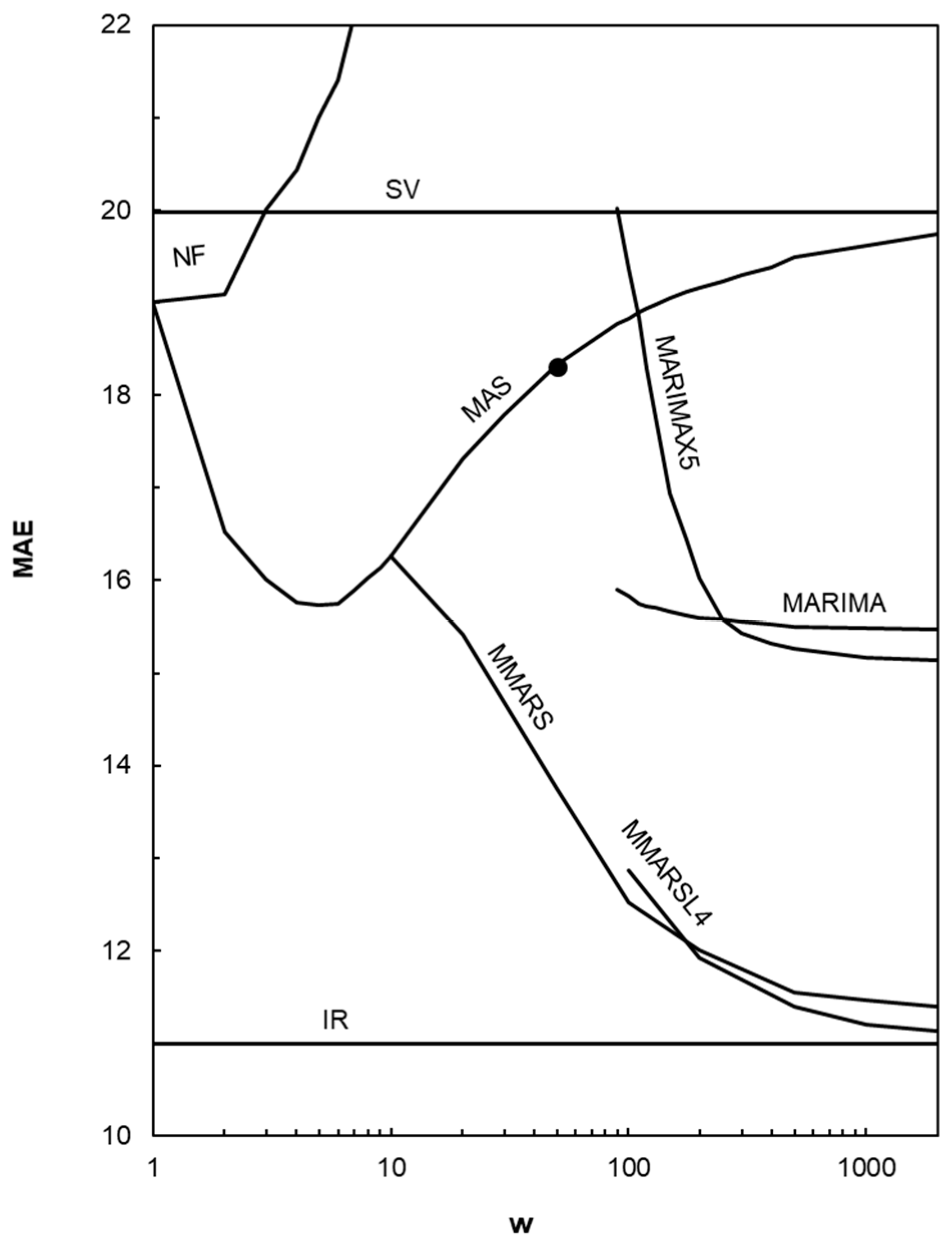
2.5.1. Stochastic Modelling

The stochastic models considered in this research are summarized in

Table 2. Stochastic models.

Model		Expression
Standard Value	SV	${\widehat{y}}_t=c_{SV}$
Naïve Forecasting	NF	${\widehat{y}}_t=y_{t-w}$
Moving Average Smoothing	MAS	${\widehat{y}}_t=\frac{1}{w}{\displaystyle {\displaystyle \sum }_{i=1}^w}{y}_{t-i}$
Auto-Regressive Moving Average with Integration	ARIMA	${\widehat{y}}_t=c+{\displaystyle {\displaystyle \sum }_{i=1}^p}{\varphi }_i{y}_{t-i}+{\displaystyle {\displaystyle \sum }_{i=1}^q}{\theta }_i{\epsilon }_{t-i}$
ARIMA with eXogenous predictors	ARIMAX	${\widehat{y}}_t=c+{\displaystyle {\displaystyle \sum }_{i=1}^p}{\varphi }_i{y}_{t-i}+{\displaystyle {\displaystyle \sum }_{i=1}^q}{\theta }_i{\epsilon }_{t-i}+{\displaystyle {\displaystyle \sum }_{i=1}^r}{\beta }_i{x}_{ti}$
Moving ARIMA	MARIMA	${\widehat{y}}_t=c^{\left(t,w\right)}+{\displaystyle {\displaystyle \sum }_{i=1}^p}{\varphi }_i^{\left(t,w\right)}{y}_{t-i}+{\displaystyle {\displaystyle \sum }_{i=1}^q}{\theta }_i^{\left(t,w\right)}{\epsilon }_{t-i}$
Moving ARIMAX	MARIMAX	${\widehat{y}}_t=c^{\left(t,w\right)}+{\displaystyle {\displaystyle \sum }_{i=1}^p}{\varphi }_i^{\left(t,w\right)}{y}_{t-i}+{\displaystyle {\displaystyle \sum }_{i=1}^q}{\theta }_i^{\left(t,w\right)}{\epsilon }_{t-i}+{\displaystyle {\displaystyle \sum }_{i=1}^r}{\beta }_i^{\left(t,w\right)}{x}_{ti}$

. They are ordered by increasing level of complexity. The Standard Value (SV) is the simplest method. The predicted temperature, $\widehat{y}$, for the actual heat, t, is given by a fixed standard value $c_{SV}$, usually the mean of all previous observations. A very cost-effective model, i.e., Naïve Forecasting (NF), takes the last registered observation, $y_{t-w}$, as the predicted temperature for the actual heat. Normally, w = 1, but it can be greater when the immediate previous temperature cannot be measured or stored. The next considered method is the Moving Average Smoothing (MAS). This method takes the average of the last w values, and presumably, gives better predictions. These very simple models are frequently employed as a benchmark, as well as a backup model in the absence of detailed process data [38].

However, when it comes to time series forecasting, the most straightforward option is AutoRegressive Integrated Moving Average (ARIMA). These models are based on the p previous observations of the predicted variable, as well as on the q previous prediction errors [39]. These models can be further improved by introducing additional r eXogenous variables $x_{ti}$, resulting in ARIMAX models [40]. The five variables indicated in Table 1, i.e., x₁, … x₅, were used as exogenous predictors in this research.

In the standard version of these models, the regression coefficients c, ${\varphi }_i$ and ${\theta }_i$ are kept constant for successive forecasts, i.e., for every t. However, to ensure long-term performance in terms of stability and consistency, the model can be retrained using the w previous observations. This results in Moving ARIMA and Moving ARIMAX models (MARIMA and MARIMAX, respectively).

2.5.2. Machine Learning

Adaptive multivariate regression models are expected to more effectively take advantage of the information contained in the exogenous predictors than the ARIMAX models. Among the multivariate regression methods, the technique known as Multivariate Adaptive Regression Splines (MARS) stands out. Since its introduction by Friedman [41,42] in the 1990s, it has been applied to various fields, including biology, medicine, finance, industry, energy and the environment.

Despite the good predictive capabilities of this technique, its first application to the BOF process was only published recently [15]. Until this contribution, the application of MARS to steelmaking processes was limited to continuous casting and rolling processes [43,44,45].

As seen in

Table 3. Machine Learning models.

Model		Expression
Multivariate Adaptive Regression Splines	MARS	${\widehat{y}}_t={\beta }_0+{\displaystyle {\displaystyle \sum }_{m=1}^M}{\beta }_m{B}_m\left({\overrightarrow{x}}_t\right)$
Moving MARS	MMARS	${\widehat{y}}_t={\beta }_0^{\left(w,t\right)}+{\displaystyle {\displaystyle \sum }_{m=1}^M}{\beta }_m^{\left(w,t\right)}{B}_m^{\left(w,t\right)}\left({\overrightarrow{x}}_t\right)$
Moving MARS with Lagged observations	MMARSL	${\widehat{y}}_t={\beta }_0^{\left(w,t\right)}+{\displaystyle {\displaystyle \sum }_{m=1}^M}{\beta }_m^{\left(w,t\right)}{B}_m^{\left(w,t\right)}\left({\overrightarrow{x}}_t, y_{t-1}, \dots y_{t-L}\right)$

, the MARS prediction is just a weighted sum of functions of the predictor variables. The ${\beta }_m$ weighting coefficients are straightforwardly obtained by regression. Regarding functions $B_m({\overrightarrow{x}}_t)$, a nonparametric adaptive technique based on domain segmentation together with a simple subset of basis functions is usually adopted [41,42,46]. A practical implementation of this technique, the ARESLAB toolbox for MatLab, has been made publicly available by Jekabsons [47].

In a similar fashion to moving ARIMA models, the standard MARS implementation was also modified by retraining the model with the w previous observations for each new prediction, resulting in Moving MARS (MMARS). Moreover, in addition to the exogenous predictors, the temperature measurements for the last L previous heats were considered as additional predictors, resulting in Moving MARS with Lagged observations (MMARSL).

Artificial Neural Network (ANN) techniques were also explored in the early days of this investigation [13]. Although good overall accuracy—similar to MARS—could be obtained, the authors found it hard to ensure a good fit in every successive retraining of the model. For this reason, ANN models were abandoned in favor of MARS-based models that provided acceptable results from the first attempts, which could be successively improved afterwards.

3. Results

The aforementioned methods were tested over 8000 heats. The mean absolute errors (MAEs) of the predictions are represented in Figure 6 as a function of the training window width w. This is a convenient choice, since the error of the hot metal temperature forecast is proportional to the increase in carbon emissions, as shown in Figure 4. Therefore, MAE reduction has a direct connection to environmental improvements. For the Standard Value (SV) method, a constant MAE of 20.0 °C was obtained. For the Naïve Forecasting (NF), the minimum MAE was 19.0 °C for w = 1, but this value rapidly increased for larger lags. In the case of the Moving Average Smoothing (MAS) the resulting MAE depends highly on the width of the training window. For w = 1, MAS reduced to NF, with the same MAE, whereas the error decreased for higher w values, reaching a minimum of 15.7 °C for w = 5. For wider w, the error increased and the MAS method tended asymptotically to the SV method. The MAE for the basic MARIMA model was 15.5 °C for w = 1000. The introduction of the five exogenous predictors (MARIMAX5) resulted in a MAE of 15.2 °C for w = 1000. Wider training windows yielded little improvement. For MMARS, the MAE was 11.4 °C for w = 2000; the introduction of four lagged terms as additional predictors (MMARSL4) further reduced the MAE of the model to 11.1 °C. Again, a wider training window yielded no further reduction of errors. Finally, the initial situation before this work is represented with a solid circle, and corresponds to a MAS model with w = 50, resulting in 18.3 °C of MAE.

Table 4. Main requirements for the considered methods.

Method	Number of Variables, N	Number of Observations, w		Earliest Result in Advance (min)
		Min.	Opt.
SV	0	0	0	inf.
NF	1	1	1	10
Initial	1	50	50	10
MAS	1	1	5	10
MARIMA	1	100	1000	10
MARIMAX5	6	300	1000	10
MMARS	5	20	2000	30
MMARSL4	9	200	2000	10
IR	1	1	1	-10

indicates the number of input variables considered for each method and the number of observations of these variables that are required to train the model; both the minimum and the optimal value for the training window are specified. These are the aspects that most affect the applicability of the model, since the more variables and observations are needed, the greater the probability that any of the necessary data will be missing.

Another aspect that affects the applicability of the model is the earliest result in advance. This is the minimum elapsed time between the moment when all the required data are available and the start of the preparation of the BOF load. The SV method, being based on a fixed prediction, presents no limitations. For the rest of the models, the advance will be determined by the moment at which the process computer receives the last necessary input variable.

Typically, the last variable to be received is the actual temperature of the previous heat. Generally, this measurement is available at least 10 min before the start of the preparation of the load. Consequently, the earliest run in advance will be 10 min before. This applies to all models except for MMARS, which uses exogenous variables only. For this case, the last variable to be received is the duration of the hot metal pretreatment, that is known approximately 30 min before.

The IR thermometry method, on the other hand, introduces a delay of at least 10 min over the desired timing for load preparation. This delay is unacceptable in many situations.

Based on this information, the applicability of each method [48] can be estimated. The applicability values are shown in

Table 5. Results for the considered methods.

Method	MAE (°C)	St. dev. of Error (°C)	Carbon Footprint Reduction (kgCO2/t)	Running Time (s)	Applicability (%)	Order i
SV	20.0	25.2	−0.9	<0.1	100	8
NF	19.3	24.3	−0.5	<0.1	99	7
Initial	18.3	22.9	0.0	<0.1	99	-
MAS	15.9	20.2	1.2	<0.1	99	6
MARIMA	15.4	19.3	1.5	0.7	95	5
MARIMAX5	15.1	19.0	1.6	1.4	93	4
MMARS	11.4	14.5	3.5	2.9	97	3
MMARSL4	11.1	14.1	3.6	3.5	87	2
IR	11	12.9	3.7	<0.1	40	1

, together with the computation time, which in no case is critical.

The expected MAE for each method and the associated carbon footprint reduction are shown in Table 5. The initially existing model, a moving average with w = 50, is indicated as a reference. The indicated errors are slightly different from those shown in Figure 6. This is due to the fact that they were obtained for a different data set, consisting of 2195 heats, that was used for the final validation of the models. The standard deviation of errors is also indicated in Table 5 for the sake of completeness.

4. Discussion

As shown in Table 5, accuracy and applicability are inversely related; the lower the MAE, the lower the applicability. However, as we will discuss below, the different methods are not mutually exclusive, but can be complementary.

Obviously, the first choice should be IR thermometry whenever possible. However, it should be noted that a valid measurement cannot always be achieved by this method, and the time advance is not sufficient in most productive situations. Consequently, a temperature estimation is only received in 40% of the cases.

For the remaining 60% of cases, the MMARSL4 model can be applied with an 87% probability, as it can be run well in advance, and the required data is generally available. In this case, the MAE will be slightly worse, i.e., 11.1 °C.

The next method to try would be MMARS that only uses exogenous variables, although the accuracy is slightly worse, with an MAE of 11.4 °C.

The process proceeds in a similar way, i.e., trying to apply the other methods in increasing order of error (MARIMAX5, MARIMA, MAS and NF), until reaching the SV method that has the worst accuracy (MAE = 20.0 °C) but with 100% applicability.

In this way, when nesting the different models in the order indicated in Table 5, a combined method with 100% applicability is obtained. The MAE of the combined method is the sum of the MAE of each method, weighted by the conditional probability of being applied since its predecessor has failed. Therefore, the expected MAE turned out to be 11.3 °C. This implies a reduction in the error, with respect to the initial situation, i.e., 7 °C (approximately 3.5 kg of CO₂ per ton of liquid steel, as shown in Figure 4). This represents an annual reduction in the carbon footprint of around 14,000 t of CO₂, estimated for an annual production of 4.0 Mt for the steel mill.

Finally, the methodological guidelines for the combined development of processes and models (CDPM) are reviewed in light of the obtained results:

• Multidisciplinary work team. Throughout this research, colleagues from different sectors have worked together: academic, R&D, process engineers and sensor suppliers.
• Long-term sustainability of achievements. Adaptive and unattended predictive models were developed. Moreover, the sequential development of these models has allowed their validation over extended periods of time.
• Analysis of different process-model alternatives. Different options for improving temperature determination were assessed. Solutions were obtained from the combined use of sensors and models subject to the requirements of the process.
• Analyses of variable importance and of data quality. The BOF thermal model made it possible to identify which variables had the greatest impact in the carbon footprint. Careful data processing was a prerequisite for developing the predictive models.
• Oriented to knowledge construction. The interest of the BOF thermal model extends beyond the present research. Likewise, the application of MMARSL models can be extended to other steel mill subprocesses.

5. Conclusions

This research successfully applied the combined development of process and models (CDPM). The interest of this approach goes beyond this application. Firstly, the development of a diagnostic model has made it possible to assess different mitigation measures. Secondly, the combination of sensors and prognostic models resulted in improved accuracy and applicability. Consequently, the superiority of the combined development of processes and models was demonstrated.

Despite considering only a few process variables, machine learning techniques succeeded in extracting relevant information from the process databases. For hot metal temperature forecasting with MARS, an accuracy close to that of IR thermometry was obtained, with a much higher applicability (87% vs. 40%).

This research has shown that process-model alternatives are not mutually exclusive, but can be complementary when judiciously nested in process computer routines. Combining measuring and modelling techniques, 100% applicability was achieved with an expected error reduction of 7 °C.

References

1. Worldsteel Steel Statistical Yearbook 2019. Available online: http://www.worldsteel.org/steel-by-topic/statistics/steel-statistical-yearbook.html (accessed on 23 April 2020).
2. ArcelorMittal Climate Action Report. Available online: https://annualreview2018.arcelormittal.com/~/ media/Files/A/Arcelormittal-AR-2018/AM_ClimateActionReport_2018.pdf (accessed on 7 December 2019).
3. McLean, A. The science and technology of steelmaking—Measurements, models, and manufacturing. Metall. Mater. Trans. B 2006, 37, 319–332. [Google Scholar] [CrossRef]
4. Mazumdar, D.; Evans, J.W. Elements of mathematical modeling. In Modeling of Steelmaking Processes; CRC Press: Boca Raton, FL, USA, 2009; pp. 139–173. ISBN 1-4398-8302-5. [Google Scholar]
5. Valentini, R.; Colla, V.; Vannucci, M. Neural predictor of the end point in a converter. Rev. Metal. 2004, 40, 416–419. [Google Scholar] [CrossRef] [Green Version]
6. Liu, H.; Wang, B.; Xiong, X. Basic oxygen furnace steelmaking end-point prediction based on computer vision and general regression neural network. Optik 2014, 125, 5241–5248. [Google Scholar] [CrossRef]
7. Iwamura, T. Breakthrough Control Technologies in the Japanese Steel Industry. SICE J. Control Meas. Syst. Integr. 2008, 1, 352–361. [Google Scholar] [CrossRef]
8. Wang, G.; Tang, L. A column generation for locomotive scheduling problem in molten iron transportation. In Proceedings of the 2007 IEEE International Conference on Automation and Logistics, Jinan, China, 18–21 August 2007; IEEE: Piscataway, NJ, USA, 2007; pp. 2227–2233. [Google Scholar]
9. Goldwaser, A.; Schutt, A. Optimal torpedo scheduling. J. Artif. Intell. Res. 2018, 63, 955–986. [Google Scholar] [CrossRef]
10. Du, T.; Cai, J.; Li, Y.; Wang, J. Analysis of Hot Metal Temperature Drop and Energy-Saving Mode on Techno-Interface of BF-BOF Route. Iron Steel China 2008, 12, 83–86. [Google Scholar]
11. Wu, M.; Zhang, Y.; Yang, S.; Xiang, S.; Liu, T.; Sun, G. Analysis of hot metal temperature drop in torpedo car. Iron Steel China 2002, 37, 12–15. [Google Scholar]
12. Liu, S.; Yu, J.; Yan, Z.; Liu, T. Factors and control methods of the heat loss of torpedo-ladle. J. Mater. Metall. 2010, 9, 159–163. [Google Scholar]
13. Díaz, J.; Fernandez, F.; Gonzalez, A. Prediction of hot metal temperature in a BOF converter using an ANN. In Proceedings of the IRCSEEME, Mieres, Spain, 25–27 July 2018; pp. 27–28. [Google Scholar]
14. Díaz, J.; Fernández, F.J.; Suárez, I. Hot Metal Temperature Prediction at Basic-Lined Oxygen Furnace (BOF) Converter Using IR Thermometry and Forecasting Techniques. Energies 2019, 12, 3235. [Google Scholar] [CrossRef] [Green Version]
15. Díaz, J.; Fernández, F.J.; Prieto, M.M. Hot Metal Temperature Forecasting at Steel Plant Using Multivariate Adaptive Regression Splines. Metals 2020, 10, 41. [Google Scholar] [CrossRef] [Green Version]
16. Díaz, J.; Fernández, F.J. Synergies in Combined Development of Processes and Models: The Cases of BOF Steelmaking and Building Energy Management. Processes. (manuscript in preparation).
17. Díaz, J.; Fernández, F.J. The impact of hot metal temperature on CO2 emissions from basic oxygen converter. Environ. Sci. Pollut. Res. 2020, 27, 33–42. [Google Scholar] [CrossRef]
18. Miller, T.W.; Jimenez, J.; Sharan, A.; Goldstein, D.A. Oxygen Steelmaking Processes. In The Making, Shaping, and Treating of Steel; AISE Steel Foundation: Pittsburgh, PA, USA, 1998; pp. 475–524. ISBN 978-0-930767-03-7. [Google Scholar]
19. Ghosh, A.; Chatterjee, A. Ironmaking and Steelmaking: Theory and Practice; Eastern economy edition; 3 print; PHI Learning: New Delhi, India, 2010; ISBN 978-81-203-3289-8. [Google Scholar]
20. Ares, R.; Balante, W.; Donayo, R.; Gómez, A.; Perez, J. Getting more steel from less hot metal at Ternium Siderar steel plant. Rev. Métallurgie–Int. J. Metall. 2010, 107, 303–308. [Google Scholar] [CrossRef]
21. Wirth, R.; Hipp, J. CRISP-DM: Towards a standard process model for data mining. In Proceedings of the 4th International Conference on the Practical Applications of Knowledge Discovery and Data Mining, Crowne Plaza Midland Hotel, Manchester, UK, 11–13 April 2000; Springer-Verlag: London, UK, 2000; pp. 29–39. [Google Scholar]
22. Mariscal, G.; Marbán, Ó.; Fernández, C. A survey of data mining and knowledge discovery process models and methodologies. Knowl. Eng. Rev. 2010, 25, 137–166. [Google Scholar] [CrossRef]
23. Barati, M. Energy intensity and greenhouse gases footprint of metallurgical processes: A continuous steelmaking case study. Energy 2010, 35, 3731–3737. [Google Scholar] [CrossRef]
24. Sun, W.; Cai, J.; Ye, Z. Advances in energy conservation of China steel industry. Sci. World J. 2013, 2013, 247035. [Google Scholar] [CrossRef] [PubMed]
25. Grip, C.-E.; Larsson, M.; Harvey, S.; Nilsson, L. Process integration. Tests and application of different tools on an integrated steelmaking site. Appl. Therm. Eng. 2013, 53, 366–372. [Google Scholar] [CrossRef]
26. Kadrolkar, A.; Dogan, N. Model development for refining rates in oxygen steelmaking: Impact and slag-metal bulk zones. Metals 2019, 9, 309. [Google Scholar] [CrossRef] [Green Version]
27. Penz, F.M.; Schenk, J.; Ammer, R.; Klösch, G.; Pastucha, K. Evaluation of the Influences of Scrap Melting and Dissolution during Dynamic Linz–Donawitz (LD) Converter Modelling. Processes 2019, 7, 186. [Google Scholar] [CrossRef] [Green Version]
28. Díaz, J. Predicción de la Temperatura del Arrabio en la Acería y Evaluación de su Impacto en las Emisiones de CO2 Mediante el Desarrollo Conjunto de Procesos y Modelos (Hot Metal Temperature Forecasting at Steel Plant and Evaluation of Carbon Emissions by Combined Development in Process and Models). Ph.D. Thesis, Universidad de Oviedo, Oviedo, Asturias, Spain, 2020. [Google Scholar]
29. Kudrin, V.A. Steelmaking; Mir Publishers: Moscow, Russia, 1985; ISBN 978-5-03-000859-2. [Google Scholar]
30. NIST Chemistry WebBook. Available online: https://webbook.nist.gov/ (accessed on 12 June 2020).
31. Kelley, K.K. Contributions to the Data on Theoretical Metallurgy; US Government Printing Office: Washington, DC, USA, 1962. [Google Scholar]
32. ENSIDESA. Curso de Formación Metalúrgica Para Jefes de Sección; ENSIDESA: Oviedo, Spain, 1985. [Google Scholar]
33. Ryman, C.; Larsson, M. Reduction of CO2 emissions from integrated steelmaking by optimised scrap strategies: Application of process integration models on the BF–BOF system. ISIJ Int. 2006, 46, 1752–1758. [Google Scholar] [CrossRef] [Green Version]
34. Williams, R.V. Control of oxygen steelmaking. In Control and Analysis in Iron and Steelmaking; Butterworths monographs in materials; Butterworths: London, Boston, 1983; pp. 147–176. ISBN 978-0-408-10713-6. [Google Scholar]
35. Kozlov, V.; Malyshkin, B.Y. Accuracy of measurement of liquid metal temperature using immersion thermocouples. Metallurgist 1969, 13, 354–356. [Google Scholar] [CrossRef]
36. He, F.; He, D.; Xu, A.; Wang, H.; Tian, N. Hybrid model of molten steel temperature prediction based on ladle heat status and artificial neural network. J. Iron Steel Res. Int. 2014, 21, 181–190. [Google Scholar] [CrossRef]
37. Papacharalampous, G.; Tyralis, H.; Koutsoyiannis, D. Comparison of stochastic and machine learning methods for multi-step ahead forecasting of hydrological processes. Stoch. Environ. Res. Risk Assess. 2019, 33, 481–514. [Google Scholar] [CrossRef]
38. Hyndman, R.J.; Athanasopoulos, G. The forecaster’s toolbox. In Forecasting: Principles and Practice; OTexts: Melbourne, Australia, 2018; pp. 47–81. ISBN 0-9875071-1-7. [Google Scholar]
39. Hyndman, R.J.; Athanasopoulos, G. ARIMA models. In Forecasting: Principles and Practice; OTexts: Melbourne, Australia, 2018; pp. 221–274. ISBN 0-9875071-1-7. [Google Scholar]
40. ARIMA Model Including Exogenous Covariates. Available online: https://es.mathworks.com/help/econ/ arima-model-including-exogenous-regressors.html (accessed on 18 April 2020).
41. Friedman, J.H. Multivariate Adaptive Regression Splines. Ann. Stat. 1991, 19, 1–67. [Google Scholar] [CrossRef]
42. Friedman, J.H.; Roosen, C.B. An introduction to multivariate adaptive regression splines. Stat. Methods Med. Res. 1995, 4, 197–217. [Google Scholar] [CrossRef]
43. Nieto, P.J.G.; Suárez, V.M.G.; Antón, J.C.Á.; Bayón, R.M.; Blanco, J.Á.S.; Fernández, A.M.D. A New Predictive Model of Centerline Segregation in Continuous Cast Steel Slabs by Using Multivariate Adaptive Regression Splines Approach. Materials 2015, 8, 3562–3583. [Google Scholar] [CrossRef] [Green Version]
44. Mukhopadhyay, A.; Iqbal, A. Prediction of mechanical property of steel strips using multivariate adaptive regression splines. J. Appl. Stat. 2009, 36, 1–9. [Google Scholar] [CrossRef]
45. Yu, W.H.; Yao, C.G.; Yi, X.D. A Predictive Model of Hot Rolling Flow Stress by Multivariate Adaptive Regression Spline. In Materials Science Forum; Trans Tech Publications: Stafa-Zurich, Switzerland, 2017; Volume 898, pp. 1148–1155. [Google Scholar]
46. Smith, P.L. Curve Fitting and Modeling with Splines Using Statistical Variable Selection Techniques; NASA: Washington, DC, USA, 1982. [Google Scholar]
47. Jekabsons, G. ARESLab Adaptive Regression Splines toolbox for Matlab/Octave ver. 1.13.0 2016. Available online: http://www.cs.rtu.lv/jekabsons/Files/ARESLab.pdf (accessed on 19 April 2020).
48. Carlsson, L.S.; Samuelsson, P.B.; Jönsson, P.G. Predicting the Electrical Energy Consumption of Electric Arc Furnaces Using Statistical Modeling. Metals 2019, 9, 959. [Google Scholar] [CrossRef] [Green Version]
Figure 1. Scope of this research: a basic oxygen furnace (BOF) and the interface with the blast furnace (BF). The key aspects to be considered in this study are shown using different font colors: main materials (black), processes (gray) and process variables (green).
Processes 08 00732 g001
Figure 2. Comparison of methodologies: (a) the original CRISP-DM workflow; and (b) modified version adopted in this research for the combined development of processes and models (CDPM).
Processes 08 00732 g002
Figure 3. Sankey diagrams representing (a) mass, (b) carbon and (c) energy flows for a standard heat (no FeSi, no anthracite, 1250 °C hot metal temperature, 1700 °C steel temperature) according to [17].
Processes 08 00732 g003
Figure 4. Effect of hot metal temperature prediction error on total carbon emissions according to [17].
Processes 08 00732 g004
Figure 5. Comparison of the hot metal temperature obtained with an IR thermometer aimed hot metal stream TIR and with disposable thermocouples dipped in hot metal ladle after transfer T. Each dot represents a heat, and is formed by the weighted average of several hot metal discharges. The TIR values were corrected for the temperature drop that occurs during transfer from the torpedo to the ladle. Linear regression is represented with a solid line. The dashed line represents TIR = T. Elaborated from [14].
Processes 08 00732 g005
Figure 6. Comparison of the mean absolute error (MAE) resulting with different methods: Standard Value (SV), Naïf Forecasting (NF), Moving Average Smoothing (MAS), Moving ARIMA (MARIMA), Moving ARIMA with 5 eXogenous predictors (MARIMAX5), Moving MARS (MMARS), Moving MARS with 4 Lagged terms as additional predictors (MMARSL4) and IR thermometry. The results are represented as a function of the width of the training window, w. The initial situation is represented with a solid circle.
Processes 08 00732 g006