Article

Dynamic Modeling and Simulation of Basic Oxygen Furnace (BOF) Operation

1
Department of Chemical Engineering, McMaster Univesity, 1280 Main Street West, Hamilton, ON L8S 4L7, Canada
2
Department of Materials Science and Engineering, McMaster Univesity, 1280 Main Street West, Hamilton, ON L8S 4L7, Canada
*
Author to whom correspondence should be addressed.
Processes 2020, 8(4), 483; https://doi.org/10.3390/pr8040483
Submission received: 28 February 2020 / Revised: 26 March 2020 / Accepted: 12 April 2020 / Published: 21 April 2020
(This article belongs to the Special Issue Process Modeling in Pyrometallurgical Engineering)

Abstract

:
Basic oxygen furnaces (BOFs) are widely used to produce steel from hot metal. The process typically has limited automation which leads to sub-optimal operation. Economically optimal operation can be potentially achieved by using a dynamic optimization framework to provide operators the best combination of input trajectories. In this paper, a first-principles based dynamic model for the BOF that can be used within the dynamic optimization routine is described. The model extends a previous work by incorporating a model for slag formation and energy balances. In this new version of the mathematical model, the submodel for the decarburization in the emulsion zone is also modified to account for recent findings, and an algebraic equation for the calculation of the calcium oxide saturation in slag is developed. The dynamic model is then used to simulate the operation of two distinct furnaces. It was found that the prediction accuracy of the developed model is significantly superior to its predecessor and the number of process variables that it is able to predict is also higher.

Graphical Abstract

1. Introduction

The Basic Oxygen Furance (BOF) is responsible for approximately 70% of the steel production worldwide [1]. A schematic diagram for the BOF in shown in Figure 1. Scrap metal and hot metal are charged to the BOF, and an oxygen jet at supersonic speed is injected from the top through the lance onto the surface of the metal bath. Some of the species in the metal bath are oxidized and form a less dense slag layer. Flux is added to prevent refractory wearing and to contribute to slag formation. Millions of metal droplets are generated at the impact zone due to the impingement of the supersonic oxygen jet on the liquid metal. Carbon in the metal droplets can react with iron oxide in the slag forming carbon monoxide [2]. Experiments using X-ray fluoroscopy have shown that gas bubbles can be formed within the metal droplet itself [2,3] and not only at the metal droplet-slag interface. Carbon monoxide and carbon dioxide are also formed due to decarburization taking place at the impact zone. The droplet-gas-slag mixture, commonly referred to as emulsion, can occupy most of the furnace volume during the main blow.
The process has limited automation and is highly dependent on operators’ knowledge and past experience. Without a framework that can consistently aid the operators with the decision-making process, some of the more complex interactions between the process variables may be overlooked, leading ultimately to sub-optimal operation. Therefore, an optimization framework for the BOF operation that can consistently provide operators with the economically optimal operating conditions could greatly help steelshops reduce production costs. However, in order to have an optimization framework it is necessary to have an accurate enough dynamic model of the physical process.
Several dynamic models [4,5,6,7,8,9] for the BOF have been developed in recent years. Jalkanen [4] developed the CONSIM 5 simulator for the BOF. All reactions are assumed to take place in one zone and oxygen is partitioned according to its affinity to a certain element. The model accounts for slag formation, energy balance, scrap melting and decarburization.
Sarkar et al. [8] also developed a dynamic model for the BOF. They assumed that the refining reactions take place only in the emulsion zone, between elements dissolved in the droplets and FeO in slag. Oxygen is distributed between the elements in the upper part of the metal bath according to their concentration. The model does not include an energy balance and temperature is assumed to increase linearly during the blow.
Another dynamic model for the basic oxygen furnace was developed by Lytvynyuk et al. [7]. All the supplied oxygen is used to form iron oxide and all other refining reactions take place via reaction with FeO. The rate of the reactions taking place in the metal bath and slag is primarily dependent on the kinetics of mass transfer. For the energy balance, the slag and metal bath are assumed to have the same temperature. The model seems to give excellent prediction of the slag composition, metal bath composition and metal bath temperature at the end of the blow.
A few dynamic models based primarily on empirical relationships have also been developed. Kattenbelt and Roffel [5] used step responses to model the decarburization rate during the main blow. They studied the process response to step changes in lance height, oxygen flow rate and iron ore addition. The model makes extensive use of empirical relationships but provides limited physical insight.
A very comprehensive, first-priniciple dynamic model for the kinetics of decarburization in the BOF was developed by Dogan et al. [6]. Their model accounts for carbon oxidation in two zones: The emulsion and the impact zone (Figure 1). At the impact zone, carbon in the metal bath is assumed to react directly with oxygen and carbon dioxide, and in the emulsion zone carbon in the metal droplets is oxidized by FeO in the slag. The metal bath and slag temperature are assumed to increase linearly with blowing time and the slag composition is required as an input. Rout et al. [9] continued the work of Dogan et al. [6] by modeling the kinetics of manganese, phosphorus and silicon oxidation enabling the model to predict the slag composition.
The current study extends the work of Dogan et al. [6] by incoporating a model for slag formation as well as energy balances. The model for decarburization in the emulsion zone is modified to account for recent fidings [10] and the model for scrap melting is updated based on recent studies [11]. The mathematical model for the BOF is implemented as a system of Differential Algebraic Equations (DAEs) using CasADi [12] with a Python front-end. The resulting framework is used to simulate the Cicutti data [13] as well as 71 heats for the BOF of an industrial collaborator (Plant A).

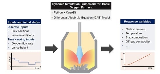
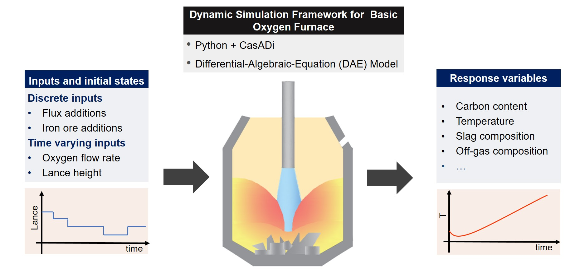
2. Mathematical Model

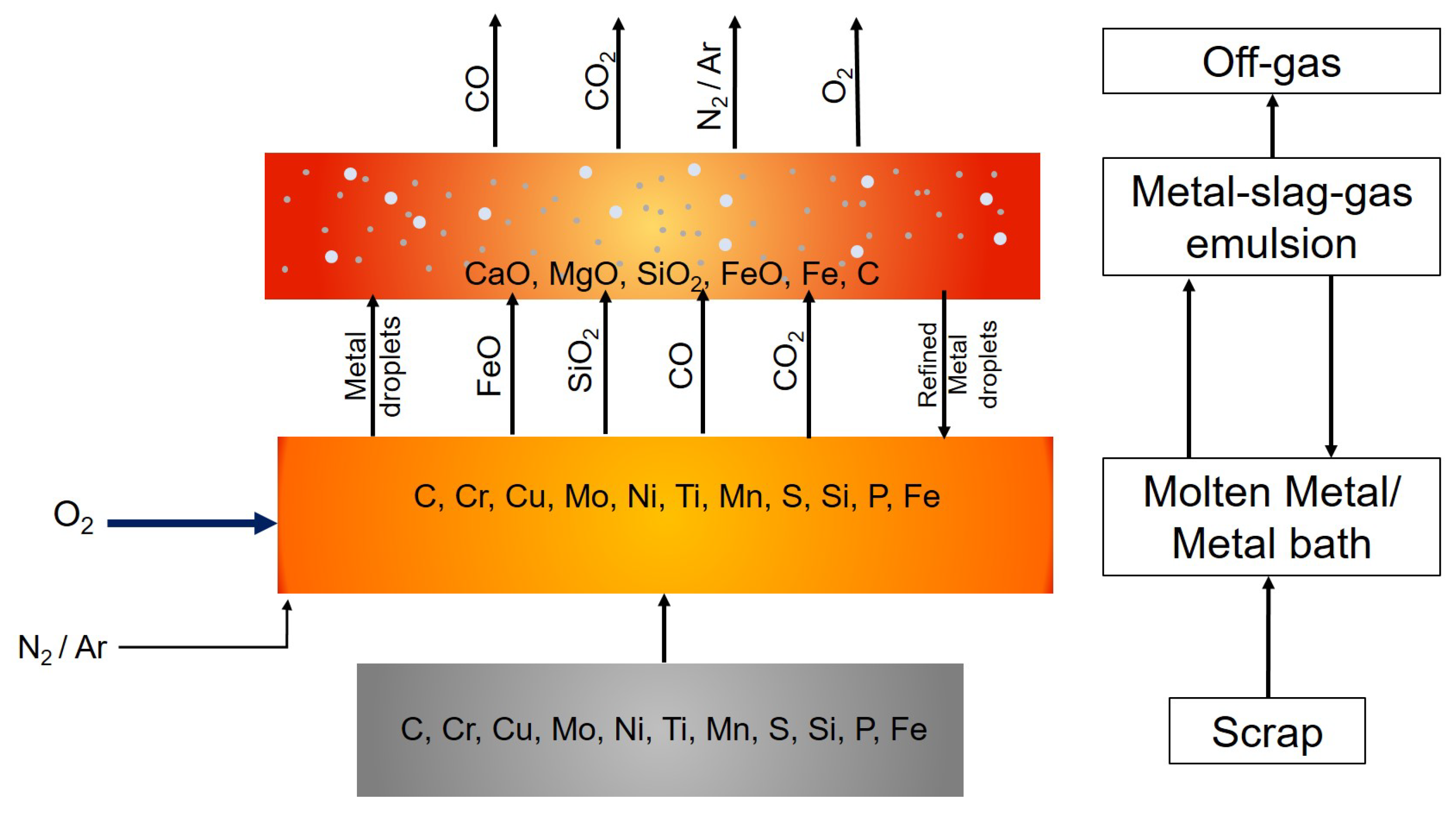
2.1. Mass and Energy Balances

The phenomena taking place in the BOF are quite complex, therefore several assumptions are made for the derivation of the mass and energy balances. Flux, iron ore, metal droplets and gas bubbles are considered to be uniformly dispersed in the slag phase. The metal droplets, gas bubbles and slag form an emulsion for which the continuous phase is assumed to be the slag. The oxidation reactions take place mainly at the impact zone (IZ), the interface between the oxygen jet and the metal bath, and there is no resistance to the diffusion of oxides from the metal bath to the slag. A schematic representation of the flow of material in the BOF is shown in Figure 2.
The reactions modelled by the current work are as follows [14], where heats of reaction, Δ H r x n , were obtained from FactSage at 1900 K:
Decarburization:
[ C ] + 1 2 O 2 ( g ) C O ( g ) Δ H r x n = 118.613 kJ / mol
[ C ] + C O 2 ( g ) 2 C O ( g ) Δ H r x n = 160.623 kJ / mol
( F e O ) + [ C ] [ F e ] + C O ( g ) Δ H r x n = 124.644 kJ / mol
Desiliconization:
[ S i ] + O 2 ( g ) ( S i O 2 ) Δ H r x n = 945.172 kJ / mol
Iron Oxidation:
[ F e ] + 1 2 O 2 ( g ) ( F e O ) Δ H r x n = 242.783 kJ / mol
Post-combustion:
C O + 1 2 O 2 C O 2 ( g ) Δ H r x n = 277.927 kJ / mol
Argon or nitrogen can be injected at the bottom of the BOF to improve mixing. Even though the injected nitrogen can undergo reaction at BOF operating conditions, the amount of nitrogen compounds formed is small and can be neglected. Therefore, it is assumed that the stirring gas leaves the furnace unreacted. At the impact zone, iron, carbon and silicon react with the injected oxygen forming iron oxide, carbon monoxide and silica as shown in Equations (1)–(5). Some of the CO may further react with O2 forming CO2 (Equation (6)).
The mass of dissolved flux and oxides is promptly incorporated by the slag. Similarly, the mass of melted scrap is assimilated by the metal bath. All Fe in the iron ore is assumed to be in the form of magnetite (Fe3O4) that is reduced to FeO by carbon in the metal bath (Equation (7)).
F e 3 O 4 + [ C ] ( 3 F e O ) + C O ( g ) Δ H r x n = 184.660 kJ / mol
The impact of the oxygen jet on the liquid metal causes millions of metal droplets to be ejected in the emulsion zone. Carbon in the metal droplets can reduce FeO in the slag according to the reaction shown in Equation (3). The refined droplets then fall back to the metal bath.
The gases CO, CO2, N2/Ar and unreacted oxygen O2 form the off-gas stream. Owing to the high temperatures, the residence time for the gases is assumed to be negligible in this work. A mass balance for the metal bath gives:
d W b d t = W ˙ s c - W ˙ C , I O + W ˙ D , e - b - W ˙ D , b - e - W ˙ C , b - e - W ˙ F e , b - e - W ˙ S i , b - e
where W b represents the mass of the metal bath. W ˙ s c is the scrap melting rate, W ˙ C , I O is the rate at which carbon in the metal bath is consumed to reduce magnetite in the iron ore to FeO, W ˙ D , b - e and W ˙ D , e - b are the mass flow rate of droplets from the metal bath to the emulsion and from the emulsion to the metal bath, respectively. W ˙ C , b - e , W ˙ F e , b - e , W ˙ S i , b - e are the mass flow rate of carbon, iron and silicon out of the metal bath and equals the oxidation rate of the respective element at the impact zone. A similar mass balance on the slag–metal–gas emulsion gives:
d W s m e d t = W ˙ D i s s F l u x + W ˙ F e O , I O + W ˙ F e O , b - e + W ˙ S i O 2 , b - e + W ˙ D , b - e - W ˙ D , e - b - W ˙ C O , E Z
where W s m e is the mass of the slag and droplets in the emulsion. W ˙ D i s s F l u x is the rate of lime and dolomite dissolution, W ˙ F e O , I O denotes the mass flow rate of iron oxide coming from iron ore, W ˙ F e O , b - e , W ˙ S i O 2 , b - e are the mass flow rate of iron oxide and silicon dioxide into the slag and are equal to the rate of formation of the respective component at the impact zone. W ˙ C O , E Z is the rate carbon monoxide is formed at the emulsion zone due to droplet decarburization.
Heat is generated in the BOF by the oxidation and post-combustion reactions (Equations (1) and (4)–(6)) and is consumed by scrap melting, to heat the fluxes and iron ore, by decarburization in the emulsion (Equation (3)) and carbon dioxide reduction (Equation (2)). The total heat Q g e n r x n generated by the oxidation reactions is given by
Q g e n r x n = Q F e O r x n + Q S i O 2 r x n + Q C O r x n + Q C O 2 r x n
where Q F e O r x n is the heat from iron oxidation (Equation (5)), Q S i O 2 r x n is the heat from silicon oxidation (Equation (4)), Q C O r x n is the net heat generation from decarburization at the impact zone (Equations (1) and (2)), Q C O 2 r x n is the heat of CO post-combustion. Q i r x n is obtained by multiplying the rate of formation of compound i at the impact zone by the respective heat of reaction.
Individual energy balances were derived for the emulsion and metal bath. To simplify the problem, the following assumptions are made:
  • The gas hold up in the slag and metal bath is negligible
  • The gas exits the furnace at the slag temperature
  • The temperature of the slag-metal-emulsion and metal bath is uniform
  • A fraction α l p of all the heat generated is assumed to be lost to the environment and the remainder is assumed to be absorbed by the slag.
An energy balance for the slag–metal–gas emulsion yields:
( W s C P , s + W D C P , b ) d T s d t = ( 1 - α l p ) Q g e n r x n - Q F e , E Z r x n - Q D , b - e - Q F e O , b - e - Q S i O 2 , b - e - Q C O , b - e - Q C O 2 , b - e - Q I O - Q e - b - Q f l u x - Q N 2 / A r , b - e - Q O 2 , b - e
with
Q i , b - e = W ˙ i , b - e C P , i ( T s - T b ) for i { F e O , S i O 2 , C O , C O 2 , N 2 / A r , O 2 }
In the above, W s is the mass of slag, W D is the mass of the droplets in emulsion, C P , s , C P , b , C P , i are the heat capacity of the slag, molten metal and component i, respectively. Q F e , E Z is the heat consumed by the decarburization reaction in the emulsion, Q D , b - e is the heat required to raise the temperature of the incoming droplets to the temperature of the slag–metal–gas emulsion; Q F e O , b - e , Q S i O 2 , b - e , Q C O , b - e , Q C O , b - e and Q C O 2 , b - e are the heat required to raise the temperature of the iron, silicon, carbon oxide and carbon dioxide formed at the impact zone to the emulsion temperature, respectively; Q e - b is the heat lost from the emulsion to the metal bath, Q f l u x and Q I O are the heat consumed by the flux and iron ore additions, Q N 2 / A r , b - e is the heat required to raise the temperature of the stirring gas from the bath to the emulsion temperature, Q O 2 , b - e is the heat required to raise the temperature of the non-reacted oxygen from the bath to the emulsion temperature. The rate of heat transfer between the slag and metal bath is given by:
Q e - b = h s - b π R 2 ( T s - T b )
where R is the furnace diameter and h s - b is the heat transfer coefficient, which can be estimated using dynamic data. Applying an energy balance for the metal bath gives:
W b C P , b d T b d t = Q e - b + Q D , e - b - Q O 2 , i n - Q N 2 / A r , i n - Q s c
where Q D , e - b is the heat transferred by the droplets coming from the emulsion to the metal bath, and Q s c is heat used to melt the scrap, Q O 2 , i n and Q N 2 / A r , i n are the heat consumed to raise the temperature of oxygen and stirring gas to the bath temperature:
Q i , i n = F i C P , i ( T b - T i , 0 ) for i { N 2 / A r , O 2 }
where F i , T i , 0 are the inlet mass flow rate and temperature of gas i.

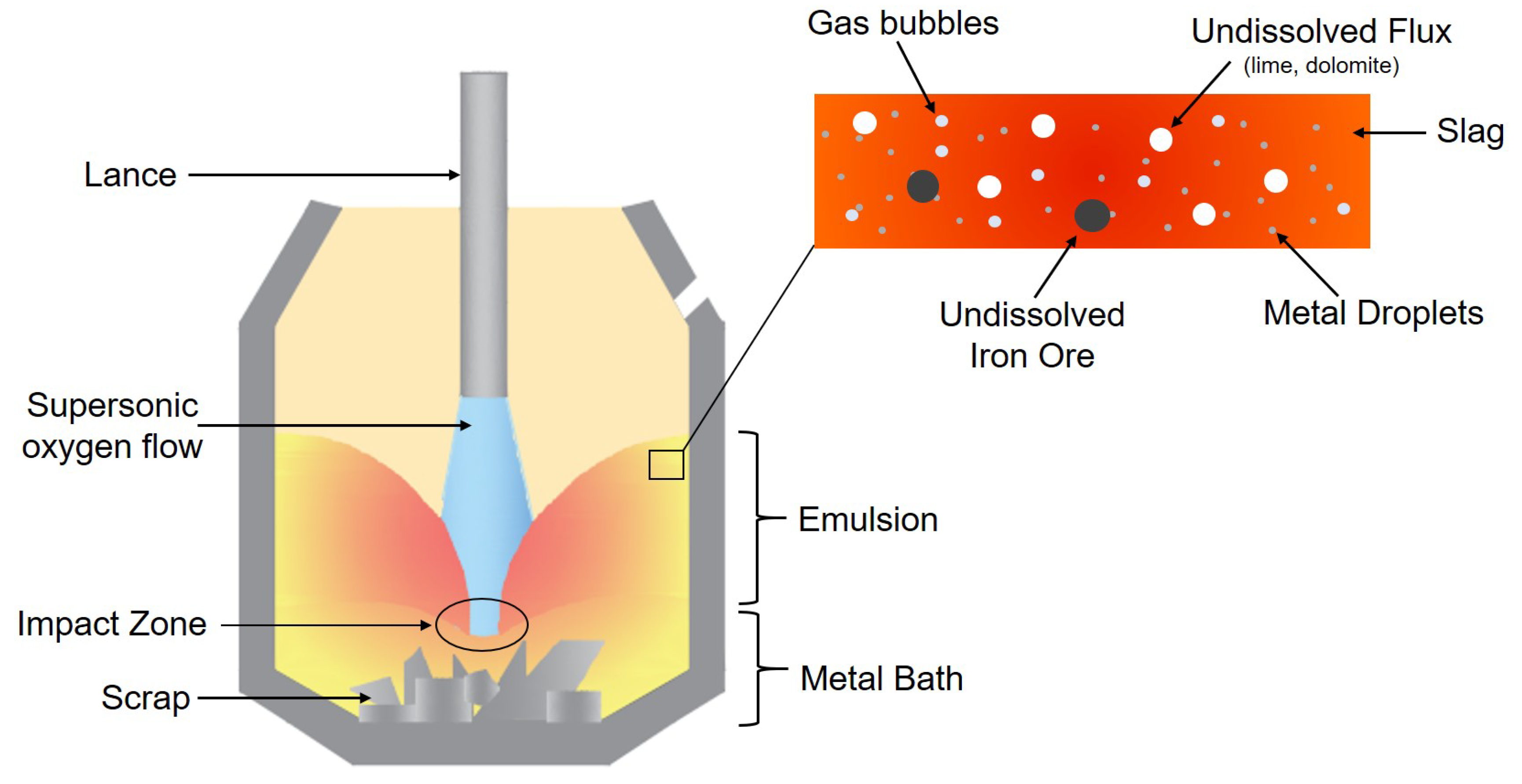
2.2. The Impact Zone
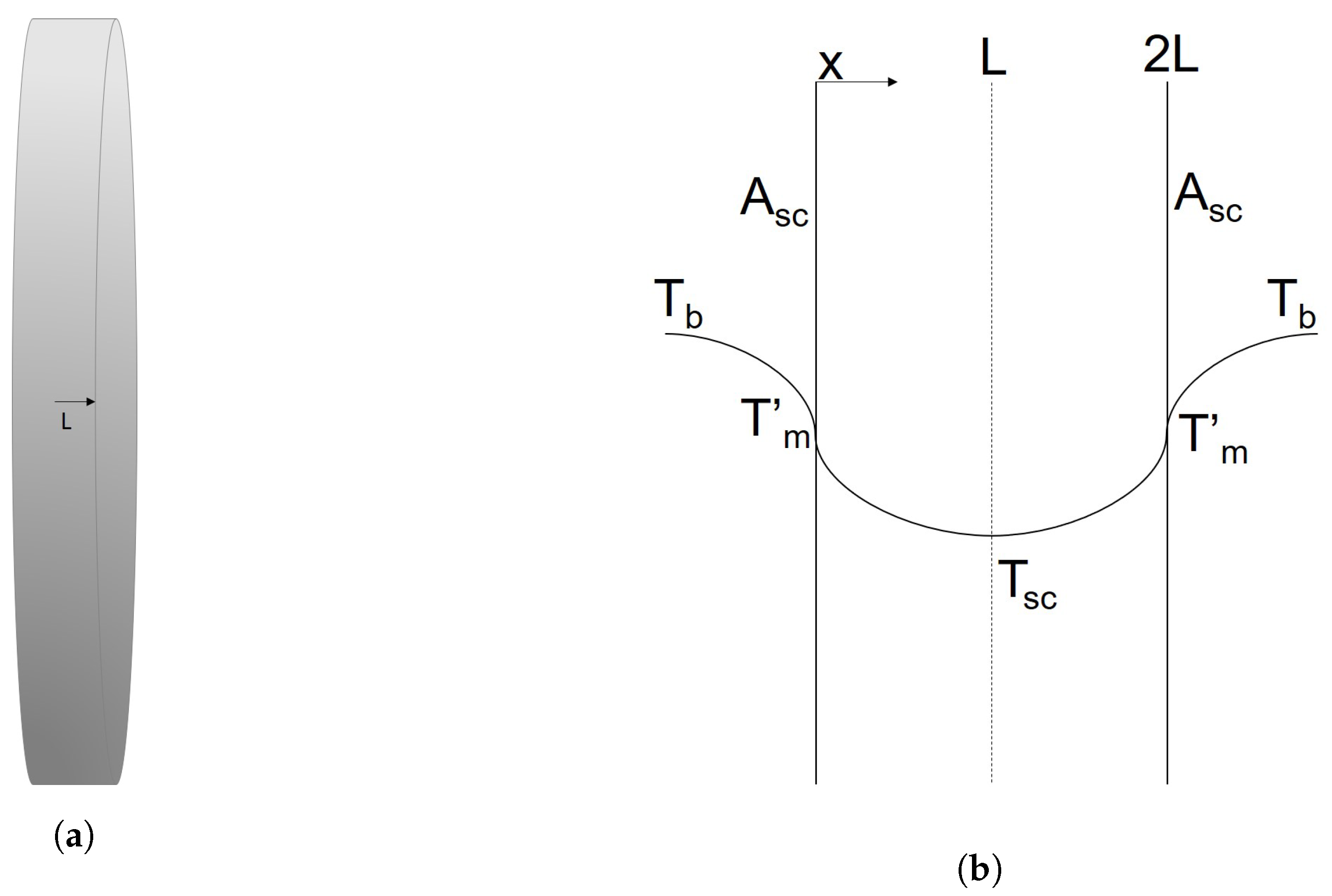
The impact zone in the BOF is the region where the oxygen jet impinges on the molten metal bath (Figure 1) causing a deformation on the liquid surface that is assumed to have the shape of a paraboloid of height h c and maximum diameter d c . The number of impact zones is equivalent to the number of nozzles n n in the lance as long as there is no coalescence of the oxygen jet. The area of one impact zone is equal to the surface area of the paraboloid:
A i z = d c π 12 h c 2 d c 2 4 + 4 h c 2 1.5 - d c 3 8
where d c and h c are calculated using the correlations proposed in [15]. For the current work, the decarburization rates previously used by Dogan et al. [6] are modified by a parameter α p in order to account for the difference between the conditions at which the equation rates were derived and the BOF operating conditions. These parameters can be tuned using process data. Therefore, the decarburization rate via O 2 (Equation (1)) is -2 r O 2 , i z , where:
- r O 2 , i z = α O 2 , t p A i z n n k O 2 ln ( 1 + P O 2 )
with:
α O 2 , t p = α O 2 p 1 + α S i , C p [ % S i ]
The partial pressure in Equation (17) is in atm, and the parameter α S i , C p in Equation (18) accounts for the inhibiting effect that silicon has on the rate of carbon oxidation [14]. Similarly, the decarburization rate via CO 2 (Equation (2)) is given by:
- r C O 2 , i z = α C O 2 p A i z n n k a P C O 2
In the above expressions, k a and k O 2 are the rate coefficients calculated using the correlations found in Dogan et al. [6] and P is the partial pressure calculated as:
P i = F i i F i P a for i { O 2 , C O , C O 2 , N 2 / A r }
where P a is the ambient pressure. In Equation (20), F O 2 and F N 2 / A r are the inlet molar flow rate of oxygen and bottom stirring gas, and F C O and F C O 2 are the molar flux of carbon monoxide and carbon dioxide formed from the decarburization reaction in Equations (1) and (2) and the post-combustion reaction in Equation (6).
When the carbon content of the metal bath [ % C ] becomes lower than the critical carbon content C C , the decarburization rate is given by [6]:
- r C c , i z = α C c p k m A i z n n V b [ % C ]
where V b is the volume of liquid metal and k m is the rate constant calculated using the correlation developed by Kitamura et al. [16].
The desiliconization rate is calculated using the expression found in Rout et al. [17] and modified by a parameter α S i p to give:
- r S i , i z = α S i p k m ρ b ( [ % S i ] - [ % S i e q ] ) A i z n n
where ρ b is the density and [ % S i ] is the silicon content of the liquid metal. Rout et al. [9] found that the equilibrium silicon content of the metal bath ( [ % S i e q ] ) is approximately zero, therefore it is neglected in the calculations. For the current study, it is assumed that the rate of iron oxidation is proportional to the partial pressure of oxygen and is given by:
- r F e , i z = α F e p A i z n n P O 2
All the oxygen injected in the system via the lance that is not used for decarburization, desiliconization or iron oxidation, is assumed to be used in the post-combustion of CO.

2.3. Scrap Melting

In the BOF, the heat generated by the oxidation reactions (Equations (1) and (4)–(6)) is much higher than that required to reach the targeted end-point temperature. Therefore, scrap metal is usually added in order to absorb part of the surplus heat via melting. In this section the model used to compute the scrap melting rate W ˙ s c as well as the heat absorbed Q s c is presented.
Consider a scrap metal plate of half-thickness L, initial temperature T s c 0 and melting temperature T m , as shown in Figure 3a.
This plate is then submerged in a metal bath at temperature T b > T m and carbon content [ % C ] . Assuming that heat transfer occurs only in the axial direction and constant physical properties for the plate, a heat balance at the interface between the solid plate and the metal bath gives [11,18,19,20]:
- k s c A s c T s c ( 0 , t ) x - h s c A s c ( T b - T m ) = d L d t ρ s c ( Δ H s c + C P , s c ( T b - T m ) ) A s c T b T m
where k s c is the thermal conductivity of the scrap plate, h s c is the heat transfer coefficient, ρ s c is the scrap density, Δ H s c is the latent heat of melting of the scrap, C P , s c is the specific heat of the scrap, A s c is the interfacial area, x is the distance of a point within the scrap from the interface, t is time and T s c ( x , t ) is the scrap temperature at a position x. A schematic representation can be found in Figure 3b.
Equation (24) can be solved using the Quasi-Static approach to yield Equations (25)–(27) [21]:
d L d t = n = 1 - A n n π ( 1 - c o s ( n π ) ) λ 2 k s c L e - λ 2 α s c t - h ( T b - T m ) ρ s c ( Δ H s c + C P , s c ( T b - T m ) ) - n = 1 A n n π ( 1 - c o s ( n π ) ) ( ρ s c C P , s c + 2 λ 2 k s c t ) e - λ 2 α s c t
λ = n π 2 L ( t )
A n = 2 ( T s c 0 - T m ) 1 - c o s ( n π ) n π
where α = k s c / ρ s c C P s c is the thermal diffusivity. The scrap melting rate W ˙ s c is then given by:
W ˙ s c = - n s c 2 ρ s c A s c d L d t
where n s c is the total number of scrap plates.
At the beginning of the BOF operation, the temperature of the molten metal may not be high enough to melt the scrap, in which case the interface temperature T m is equal to the bath temperature T b . The interface temperature is otherwise assumed to correspond to the melting temperature. This is shown in Equation (29):
T m = T b T b < T m T m T b T m
The melting temperature T m is dependent on the carbon content C m at the melting interface and can be calculated using Equation (30) [22]:
T m = 1810 - 90 % C m 0 % C m 4.27 % 1425 % C m > 4.27 %
Dogan [22] assumed C m to be equal to the carbon content in the bulk metal [ % C ] . This assumption reflects, to some extent, what happens in the BOF: Carbon in the metal bath migrates to the scrap surface lowering its melting temperature [21,23]. One consequence of such an assumption is that scrap types of similar physical properties will all melt at the same time, independent of their carbon content. On the other hand, if C m is assumed to be equal the carbon content of the scrap C s c , low-carbon content scrap types will only melt towards the very end of the blow, which is not observed in practical BOF operations. For the current work, C m is defined as:
C m = 0.8 [ % C ] + 0.2 C s c
The heat transfer coefficient h s c in Equation (25) is calculated according to the correlation proposed by Gaye et al. [24] and given by:
h s c = 5000 ϵ ˙ 0.2
where ϵ ˙ is the mixing power due to bottom stirring and top blowing in Wm - 3 , and h s c is in units of Wm - 2 K - 1 . The rate Q s c at which heat is absorbed by the scrap is given by the heat conduction term in Equation (24) before melting starts, and by the convective term once melting starts as shown in Equation (33).
Q s c = 2 n s c A s c - T s c ( 0 , t ) x T b < T m h ( T b - T m ) T b T m

2.4. Iron Ore Dissolution

Some steel shops also add iron ore before or during the blow to cool down the metal bath and meet the desired end point temperature. Since the mass of iron ore added is usually small compared to the amount of scrap, a rather simple model is used to account for the cooling effect of iron ore.
Iron ore composition can vary greatly according to the region but the predominant element is usually Fe followed by oxygen. For the current model all Fe in the iron ore is assumed to be in the form of magnetite (Fe 3 O 4 ) that is reduced to iron oxide by carbon in the metal bath according to Equation (7). Furthermore, the iron ore melting point T m is considered to be equal to the FeO melting point (1644 K). Reduction of magnetite and melting of the formed iron oxide are assumed to happen concomitantly. The iron ore particles are assumed to be spherical and to have uniform temperature, therefore the total heat transfered to the surface of an iron ore particle can be calculated using Equation (34):
Q c o n v , o r e = 4 π r o r e 2 h o r e ( T s - T o r e )
where T o r e is the iron ore temperature, h o r e is the heat transfer coefficient, r o r e is the radius and T s is the slag temperature. It is assumed that a fraction T o r e / T m of the total heat Q c o n v , o r e contributes to melting of the iron ore and the remainder is used for sensible heating. A similar approach was used by MacRosty and Swartz [25] and Bekker et al. [26] to model scrap melting in electric arc furnaces. At the beginning of the process T o r e < < T m and most of the heat is used to heat up the iron ore. As T o r e approaches T m , the fraction of the total heat used for melting increases. An energy balance for a single iron ore particle yields:
W o r e C P , o r e d T o r e d t = ( 1 - T o r e / T m ) Q c o n v , o r e
where W o r e is the mass of a single iron ore particle and can be obtained from Equation (36):
W o r e = 4 3 π r o r e 3 ρ o r e
In the above, ρ o r e is the iron ore density and C P , o r e is the iron ore heat capacity. A heat balance at the interface of the iron ore particle gives Equation (37) for the rate of dissolution of an iron ore particle:
A o r e ρ o r e ( Δ H o r e + C p F e O ( T s - T o r e ) ) d r o r e d t = - ( T o r e / T m ) Q c o n v , o r e
where Δ H o r e is the latent heat of melting of FeO, C P , F e O is the heat capacity of iron oxide and A o r e is the area of the interface, here equal to the surface area of a sphere of radius r o r e .
The heat consumed to reduce magnetite to iron oxide is given by:
Q r e d , o r e = y F e , o r e 3 M F e W ˙ o r e , m e l t Δ H r x n
where y F e , o r e is the mass fraction of Fe in the iron ore, Δ H r x n is the heat for the reaction defined in Equation (7), M F e is the molar mass of iron and W ˙ o r e , m e l t is the melting rate of iron ore given by:
W ˙ o r e , m e l t = 4 π ρ o r e r o r e 2 d r o r e d t
The total heat consumed by iron ore melting and reduction is given by:
Q I O = n o r e ( Q c o n v , o r e + Q r e d , o r e )
where n o r e is the number of iron ore lumps.

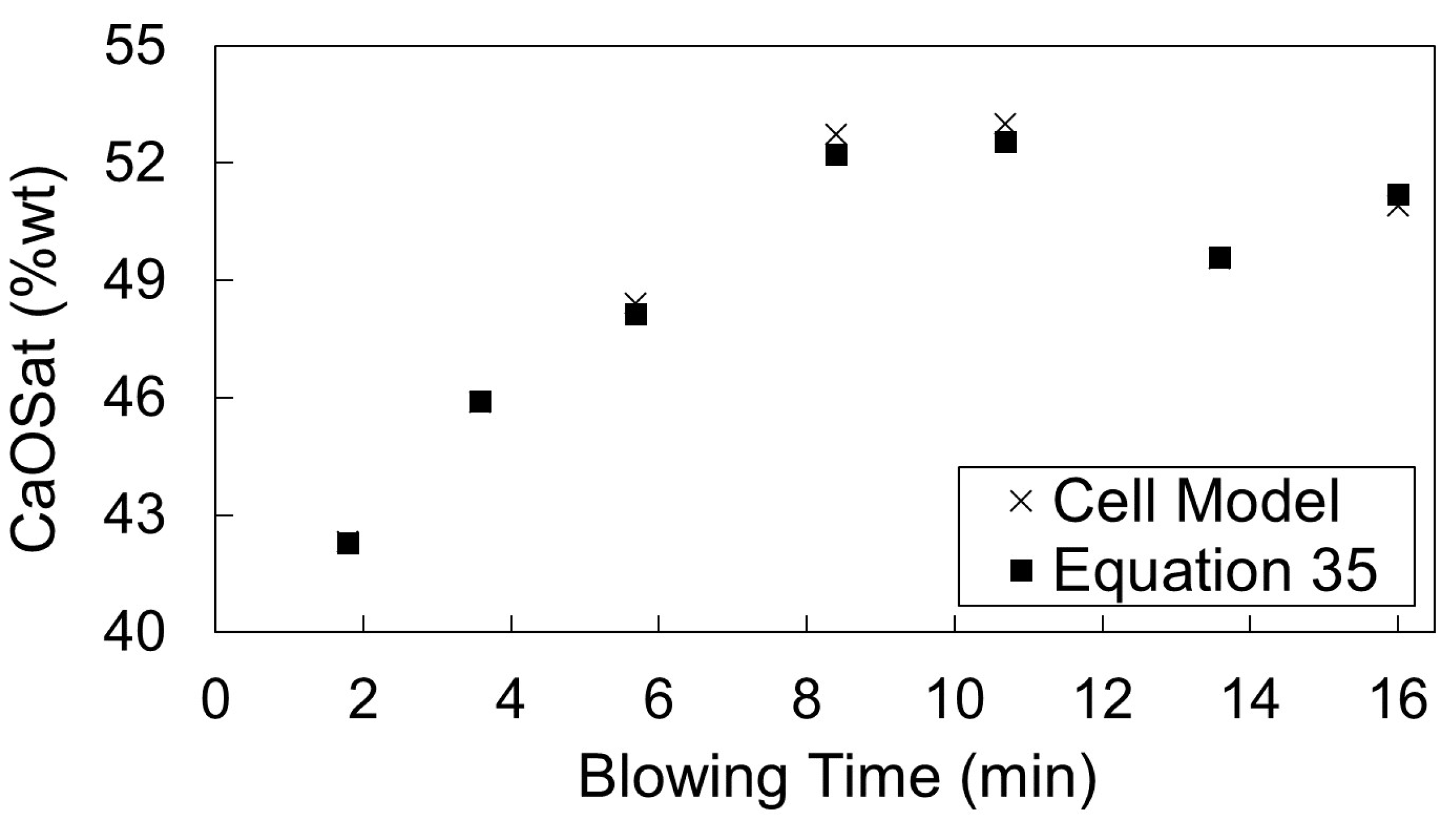
2.5. Flux Dissolution

Similarly to the decarburization rates at the impact zone, flux dissolution is modelled after Dogan et al. [27]. The flux particles are assumed to have a spherical shape, and the rate of flux dissolution is proportional to the rate of change of the particles’ radius.
The rate of lime dissolution is given by Equation (41) [27,28], where r L is the particle radius, (%CaO) is the concentration of CaO in slag, ( % C a O s a t ) is the saturation concentration of CaO in the slag, k L is the mass transfer coefficient, ρ s and ρ L are the slag and lime density, respectively. The parameter α L p is introduced here to account for deviations between the experimental conditions at which k L was derived, and the BOF operating conditions.
d r L d t = α L p k L ρ s 100 ρ L ( ( % C a O ) - ( % C a O s a t ) )
For dolomite, the rate of dissolution is given by [27,29]:
d r D d t = α D p k D ρ s 100 ρ D 1 + M M g O M C a O ( ( % C a O ) - ( % C a O s a t ) ) ( % F e O ) < 20 % α D p k D ρ s 100 ρ D 1 + M C a O M M g O ( ( % M g O ) - ( % M g O s a t ) ) ( % F e O ) 20 %
where M M g O and M C a O are the molar mass of MgO and CaO, respectively, (%MgO) is the concentration of MgO in slag, ( % M g O s a t ) is the saturation concentration of CaO in the slag and k D is the mass transfer coefficient. The rate constants k L and k D are calculated using the correlations proposed by Dogan et al. [27] with the parameter used to modify the Reynolds number β set to the nominal value of 1.
Data for the calcium oxide saturation in slag ( % C a O s a t ) for different slag compositions were obtained using the Cell Model [30], a Matlab program that gives the saturation concentration of the individual species in the slag as a function of composition and temperature. Kadrolkar et al. [30] validated the Cell Model results against FactSage T M and ThermoCalc T M . The function ’fitnlm’ in Matlab was then used to fit a curve to the generated data, yielding Equation (43).
( % C a O ) s a t = 3.52 T s - 4 , 823.7 e - 2.93 100 ( % S i O 2 ) + 12.4 ( % F e O ) - 9.71 ( % M g O ) + 17.9 ( % C a O ) 100
An R 2 of 0.9 was obtained for the nonlinear regression. The goodness of Equation (43) to predict the calcium oxide saturation in slag was evaluated using the Cicutti data [13]. The calculated values for C a O s a t using the Cell Model and Equation (43) are shown in Figure 4, where it can be seen that there is excellent agreement between them.
The rate at which heat is absorbed by the flux particles is given by:
Q f l u x = 4 π i r i 2 h i n i ( T s - T i ) i { L , D }
where T s is the temperature of the slag, T i is the flux temperature, h i is the heat transfer coefficient determined using data and n i is the number of flux particles. Assuming a uniform temperature for the flux particle, an energy balance gives Equation (45) for the temperature of an iron ore particle:
W i C P , i ρ i d T i d t = 4 π r i 2 h i ( T s - T i ) i { L , D }
where C P , i is the heat capacity and W i = 4 / 3 ρ i π r 3 is the mass of one single flux particle.

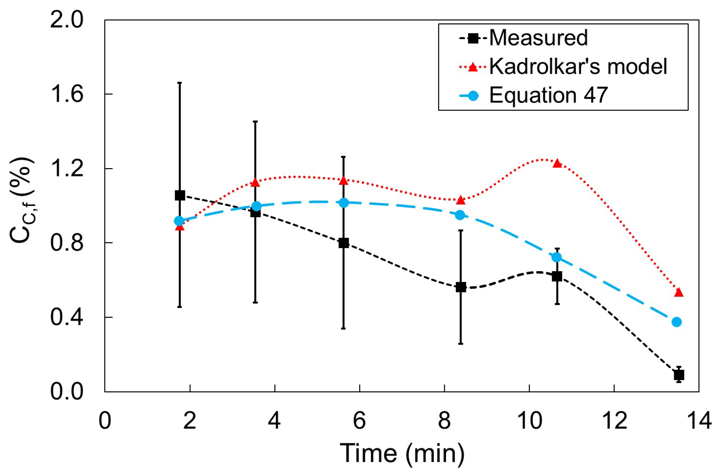
2.6. Decarburization in the Emulsion Zone

In Figure 5, the initial carbon composition and diameter of a metal droplet are represented by C i , 0 and D 0 , respectively. The metal droplet is formed from the interaction of the oxygen jet and the metal bath at the impact zone at time t 0 , and ejected to the slag–metal–gas emulsion. The droplet stays in the emulsion zone for R t seconds, then it returns to the metal bath at time t 0 + R t having a composition C i , f and diameter D f . While in the emulsion zone, carbon in the metal droplet can reduce FeO in slag according to reaction 3.
The droplet generation rate R B , given by Equation (46), is calculated using the empirical expression proposed by Subagyo et al. [31] modified by a parameter p D G to account for possible differences between the conditions at which the correlation was derived and a given BOF operation:
R B = p D G V ˙ O 2 N B 3.2 ( 2.6 × 10 6 + 2 × 10 - 4 N B 12 ) 0.2
where V ˙ O 2 is the volumetric flow rate of oxygen and N B is the blowing number [31].
Since millions of droplets are generated at every point, it can become computationally expensive to track the composition of the individual metal droplets. Therefore, an algebraic equation to calculate the final carbon content of the metal droplets was developed and the following assumptions were made in order to make the problem tractable:
  • All droplets decarburize immediately after they are ejected from the impact zone
  • The carbon content of the metal droplets in the emulsion zone is approximated as the average carbon content of the individual metal droplets
  • Except for carbon, the mass of other elements in the metal droplets stays constant whilst the droplet travels through the emulsion zone
The first-principles model developed by Kadrolkar and Dogan [10] for the droplet decarburization was used to generate data for the final carbon content ( C C , f ) of individual droplets with respect to its initial carbon content C C , 0 , the slag temperature T s and composition. Data were generated for the range of initial carbon content between 0.3% and 5% and slag temperature of 1623–2153 K, and for the slag composition provided by Cicutti et al. [13]. Equations (47) and (48) give a good description of the generated data with an R 2 of 0.96 and 0.92, respectively.
Δ C C = C C , 0 - C C , f = 0.9514 0.001 T s C C , 0 - 1.4345 ( % F e O ) > 10
C C , f = 0.67492 C C , 0 1.2261 C C , 0 / ( % F e O ) ( % F e O ) 10
In Figure 6, the average final carbon content of the droplets reported by Cicutti et al. [13], the values predicted by Kadrolkar and Dogan [10]’s model and what was obtained using Equation (47) are shown. Similar to the first-principles model proposed by Kadrolkar and Dogan [10], the final carbon content of the droplets predicted by Equation (47) is largely within the range of values reported by Cicutti [13] for a real BOF operation. These results indicate that Equation (47) approximates the kinetics of droplet decarburization reasonably well and can therefore be used within the BOF model to describe the kinetics of decarburization in the emulsion zone.
Using Equations (47) and (48) and the previously stated assumptions, and introducing a term α μ , D p to account for changes in the slag viscosity, it is possible to obtain Equation (49) for the rate of carbon removal:
W ˙ C , s = R B 1 - 1 - 0.01 C C , 0 1 - 0.01 C C , f α μ , D p
with α μ , D p given by:
α μ , D p = exp ( - α μ p μ s )
where W ˙ C , s is the rate of carbon removal, α μ p is a parameter and μ s is the slag viscosity. The initial carbon content of the droplet C C , 0 is equal to the carbon content of the metal bath C b at the time of ejection. The term α μ , D p is necessary because the effect of slag viscosity is not taken into account in Equations (47) and (48). However, it is likely that the high slag viscosity at the beginning of the blow significantly decreases the decarburization rate. At high viscosities the slag becomes less fluid, negatively impacting the rate of FeO mass transfer to the droplet surface and potentially leading to FeO depletion in the neighborhood of the droplet, decreasing the decarburization rate. The value of α μ p can be determined using dynamic data.
The mass of carbon W C , s in the emulsion is then given by:
d W C , s d t = ( 0.01 R B C C , 0 - W ˙ C , s ) 0.01 C ¯ C , s W D , s R t
where the first term on the right hand side is the amount of carbon entering the emulsion zone minus the carbon removed via decarburization, and the second term is the flow rate of carbon returning to the metal bath. C ¯ C , s is the average carbon content of the droplets in the emulsion calculated by:
C ¯ C , s = 100 W C , s W D , s
and W D , s is the total mass of droplets in the emulsion determined as:
d W D , s d t = ( R B - W ˙ C , s ) - W D , s R t
The droplet residence time R t is calculated using the following empirical expression:
R t = 5 + 20 e - 0.3 ( % F e O ) C C , 0
As long as the residence time R t of the droplets in the emulsion is small, C ¯ C , s is approximately equal to C C , f and the simplifying assumption of uniform carbon content for the droplets in the emulsion does not significantly impact the final result, while avoiding the need to track the behavior of individual droplets.

2.7. Implementation

The mathematical model presented in the previous sections was implemented as a DAE system using CasADi [12] with Python 3.7. An index-1 DAE in semi-explicit form can be written in the form given by Equations (55) and (56):
x ˙ ( t ) = f ( x ( t ) , z ( t ) , u ( t ) , p )
0 = h ( x ( t ) , z ( t ) , u ( t ) , p )
where f and h are the differential and algebraic functions, respectively, x and z are the differential and algebraic states, u and p represent the control variables and time-independent parameters, and t is time. Within CasADi, the DaeBuilder class was selected since it is capable of performing model reduction by eliminating algebraic variables that can be explicitly calculated. The resulting DAE system was solved using the variable step size DAE solver IDAS [32]. For implementation of the mathematical model, the following modifications were made where necessary:
  • Equations of the form:
    y ( a ) = 1 a
    where a 0 , were rewritten as:
    y ( a ) = 1 a + ϵ
    where ϵ is a positive small number. This strategy was used on the submodels for flux dissolution, iron ore and scrap melting to prevent division by zero since either the radius or thickness of the particles continuously decreases with time and can eventually equal zero.
  • Piecewise functions of the form:
    y ( c ) = y 1 ( c ) a > b y 2 ( c ) a b
    were rewritten using hyperbolic tangent functions:
    y ˜ ( c ) = y 1 ( 0.5 tanh ( γ ( a - b ) ) + 0.5 ) + y 2 ( 0.5 tanh ( γ ( b - a ) ) + 0.5 )
    where γ is an adjustable parameter that controls the steepness of the continuous switching function approximation. This was used for flux dissolution (Equation (42)), scrap melting (Equation (29)), decarburization in the emulsion zone (Equations (47) and (48)), among others for a smooth transition and to ensure differentiability.
  • Flux additions: Flux and iron ore can be added at anytime during a blow, and each individual addition is modeled as shown in Section 2.5. To model the indiviudal flux additons a new variable t i j , where i is the flux type (lime, dolomite, iron ore) and j is the addition number (first, second, third), is defined for the flux addition time. Given the radius r i j of the flux added at time t i j , Equation (41) for lime dissolution rate can be reformulated as:
    d r i j d t = 0 t < t i j k L ρ s 100 ρ L ( % C a O s - % C a O s a t ) t t i j
    which was implemented using a hyperbolic tangent function.

3. Results and Discussion

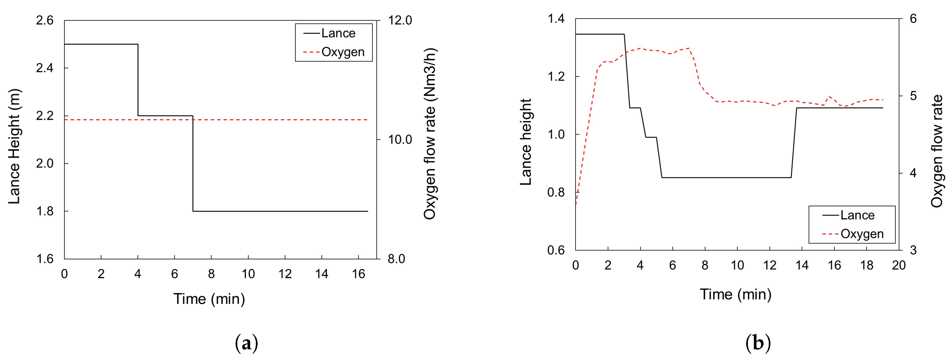
3.1. System Parameters and Input Data

The parameters α p introduced during the model development to account for distinct BOF operations and differences between the conditions at which the respective equations were derived and the operating conditions were manually adjusted for a data set available in the literature for a 200 ton furnace [13], as well as for the data provided by Plant A for 70 heats for a 250 ton furnace. The final values of the parameters α p are given in Table 1.
In Cicutti et al. [13]’s study, lime is added before the blow starts and at every minute up to 7 min, whereas dolomite is added before the blow starts and again at 7 min. Ar/N 2 gas is continuously injected from the bottom of the furnace to aid with stirring. In Plant A operations, lime and dolomite are added only before the blow starts, scrap selection varies for each heat, and the furnace design does not allow for bottom stirring.

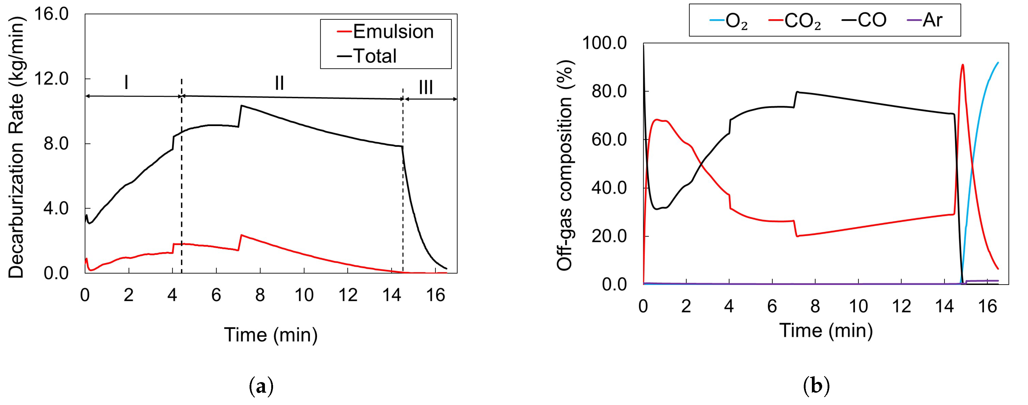
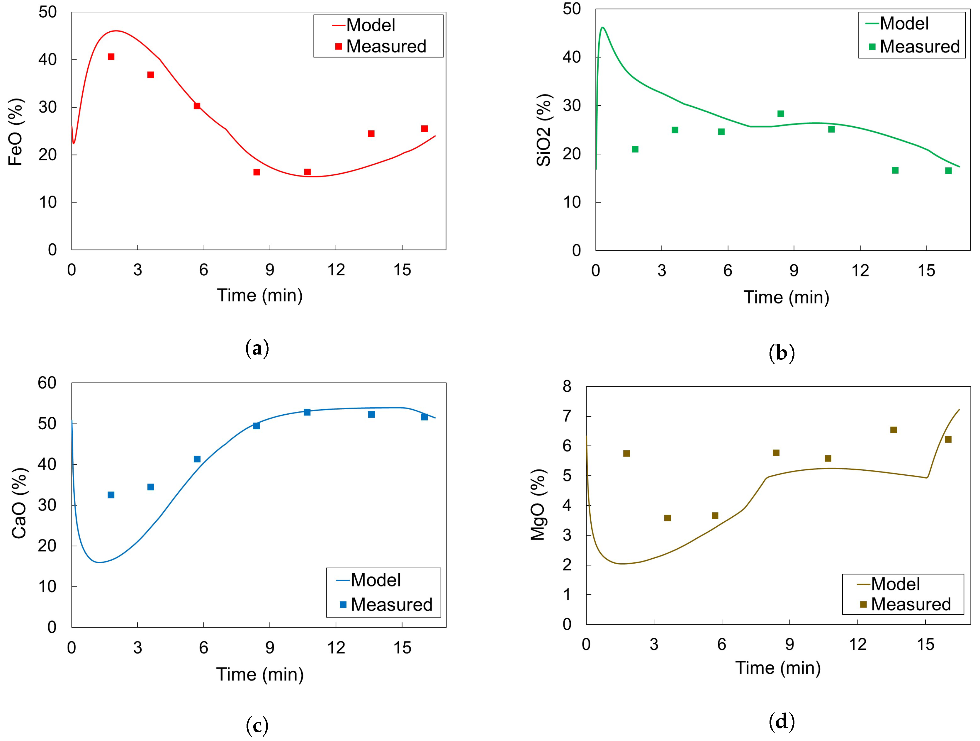
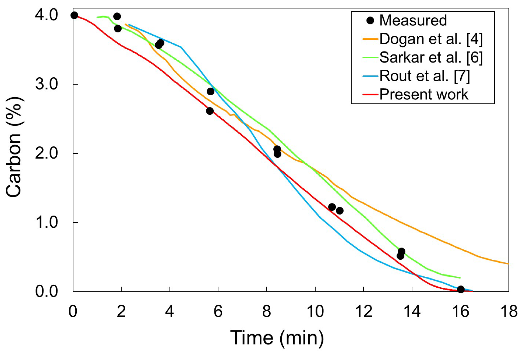
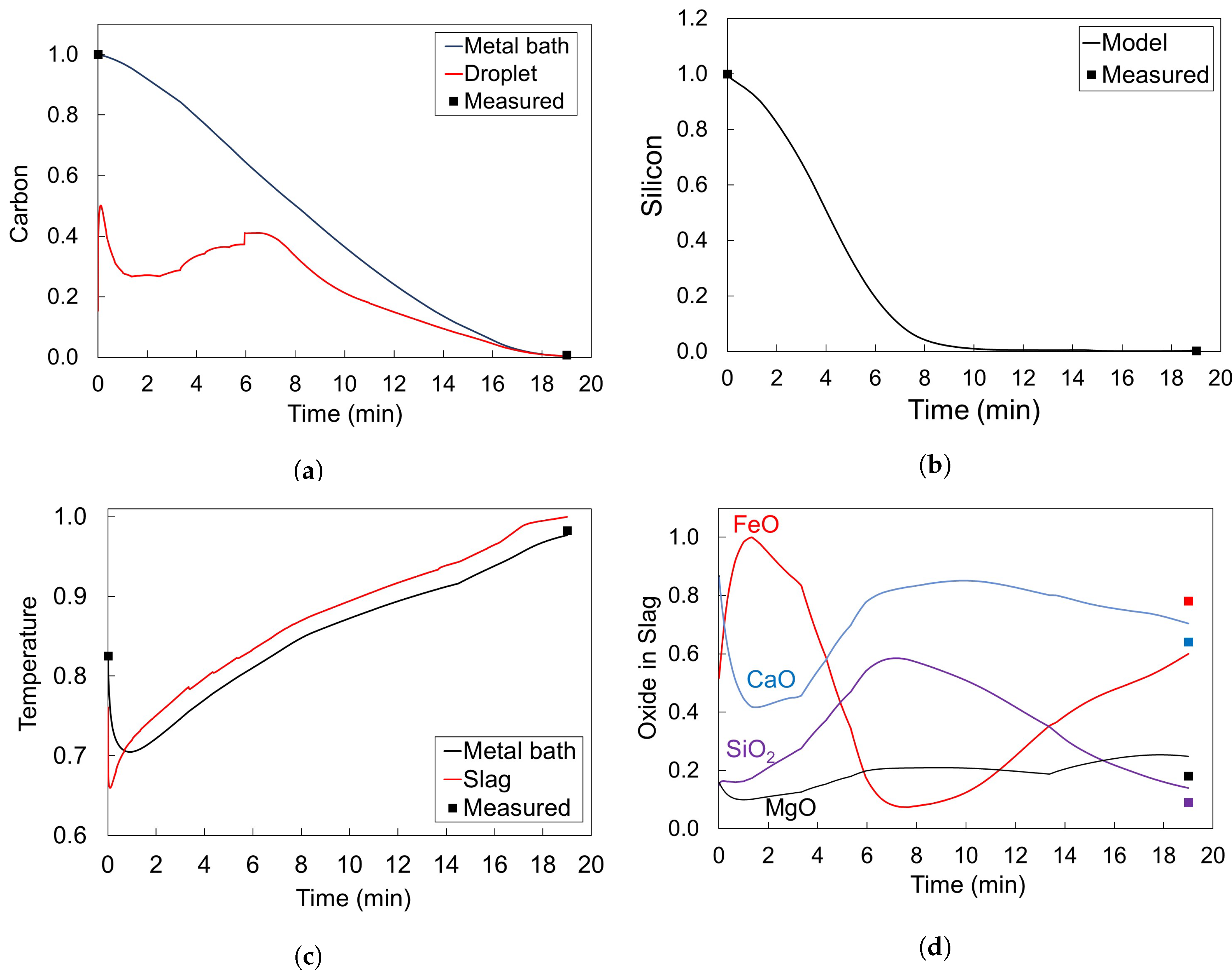
3.2. Simulation Results for Cicutti’s Operations

Cicutti et al. [13]’s data have been used to validate several dynamic models developed for the BOF [6,8,9,33]. Information regarding the hot metal and scrap compositions is shown in Table 2. For the mass of flux, gravel and iron ore refer to Cicutti et al. [13].
Figure 7 shows the metal bath temperature and carbon content predicted by the model described in this article, as well as the data published by Cicutti et al. [13].
In the first few minutes, the bath temperature decreases due to the heat absorbed by the scrap. Thereafter, the temperature increases approximately linearly as heat is released by the oxidation reactions. The oscillations in the slag temperature during the first half of the blow are due to the flux additions, done at every minute. Figure 7b shows that the carbon content predicted by the model for the bulk metal agrees well with the measured data. The predicted final carbon content of the returning droplets is also shown in Figure 7b. Due to the high interfacial area, the rate of carbon refining at the droplet level is significantly higher than that for the bulk metal, thus the lower carbon content.
The decarburization rate in the emulsion zone is shown in Figure 8a. The extent of droplet decarburization is primarily dependent on the initial carbon content of the liquid metal droplet when it is ejected from the impact zone [10]. At low initial carbon contents the liquid metal droplets do not bloat and their residence time in the emulsion zone decreases significantly [10,34]. Due to that the contribution of the emulsion zone to the total decarburization rate decreases significantly towards the end of the blow. It follows that at high carbon contents it is possible to increase the decarburization rate in the emulsion zone by increasing the droplet generation rate.
It is possible to identify the three decarturization periods characteristic of the BOF operation on the total decarburization rate graph shown in Figure 8a:
  • Period I: As the silicon content of the metal bath decreases, the decarburization rate increases
  • Period II: Decarburization rate stays approximately constant
  • Period III: Decarburization rate is controlled by mass transfer of carbon in the metal bath
The change from Period II to III is shown by the dashed line in Figure 8a, but it can also be seen in the compostion of the gases exiting the furnace in Figure 8b. As the decarburization at the impact zone decreases, more oxygen becomes available for the post-combustion reaction explaining the increase in the percentage of CO 2 at approximately 14 min. The percentage of CO 2 in Figure 8b is slightly higher than would normally be observed in practice. This can be due to the ideal assumption that all the oxygen not used in the oxidation reactions is consumed in the post-combustion of CO.
The profile for the lance height and oxygen flow rate is shown in Figure 9a. The effect of lance height changes on the decarburization rate is clear at 4 min and 7 min in Figure 8a: Lowering the lance height increases the droplet generation rate, as well as the rate constants for the decarburization reactions taking place at the impact zone, which leads to a higher decarburization rate.
The contribution of the decarburization in the emulsion to the total decarburization is significantly lower for the present work than previously suggested [8,17]. Rout et al. [17] suggested that 76% of the total decarburization happens in the emulsion, while in the modeling approach adopted by Sarkar et al. [8] decarburization only takes place in the emulsion zone. For the current paper, the emulsion zone was responsible for 15% of the total carbon removed. The reason why the contribution of the decarburization in the emulsion is lower for the present study is because of the significantly lower droplet generation rate R B . Sarkar et al. [8] modified the droplet generation rate (Equation (46)) by a factor of 15. Using a modified correlation for R B , Rout et al. [35] obtained a droplet generation rate similar in magnitude to Sarkar et al. [8]. It is not currently viable to measure how much decarburization occurs at the impact and emulsion zones individually, and it may be the case that a different set of parameter values yields approximately the same total decarburization rate. However, taking into account the gradual decrease in the decarburization rate in the emulsion zone in Figure 8a, it can be inferred that for a very high contribution of the emulsion to the total decarburizaton rate, Period II would no longer be characterized by an approximately constant decarburization rate.
The slag composition throughout the blow is presented in Figure 10 for SiO 2 , CaO, FeO and MgO. There is a good agreement between the values predicted by the model and the data. The large content of silicon dioxide in the slag during the first minute is due to 800 kg of gravel addition. A large SiO 2 content increases the slag viscosity, reducing the decarburization rate at the emulsion and allowing FeO to build up. Flux dissolution slows down significantly at high slag viscosities, but as the blow proceeds SiO 2 gets diluted by FeO and the flux dissolution rate increases. The error between the model prediction and measured data is, most likely, due to the treatment of slag as a homogeneous phase for the density and viscosity calculations [36].
A comparison between the carbon content prediction by the present and previous [6,8,9] studies is shown in Figure 11. Only for the current model, the carbon content prediction starts from time zero, and enregy balances are included; moreover, the quality of the prediction itself is quite good compared with previous works. This is also the only study for which the mathematical model was transposed as a DAE system and integrated using a variable step size solver, whilst in the aforementioned works integration was carried out using a fixed step size. The first main benefit stemming from the current implementation is the reduced computational time as shown in Table 3. Moreover, the convergence is taken care of by the integrator, and convergence studies based on step size are not required. Secondly, the dynamic model can be easily built within an optimization framework to determine the optimal input trajectories.

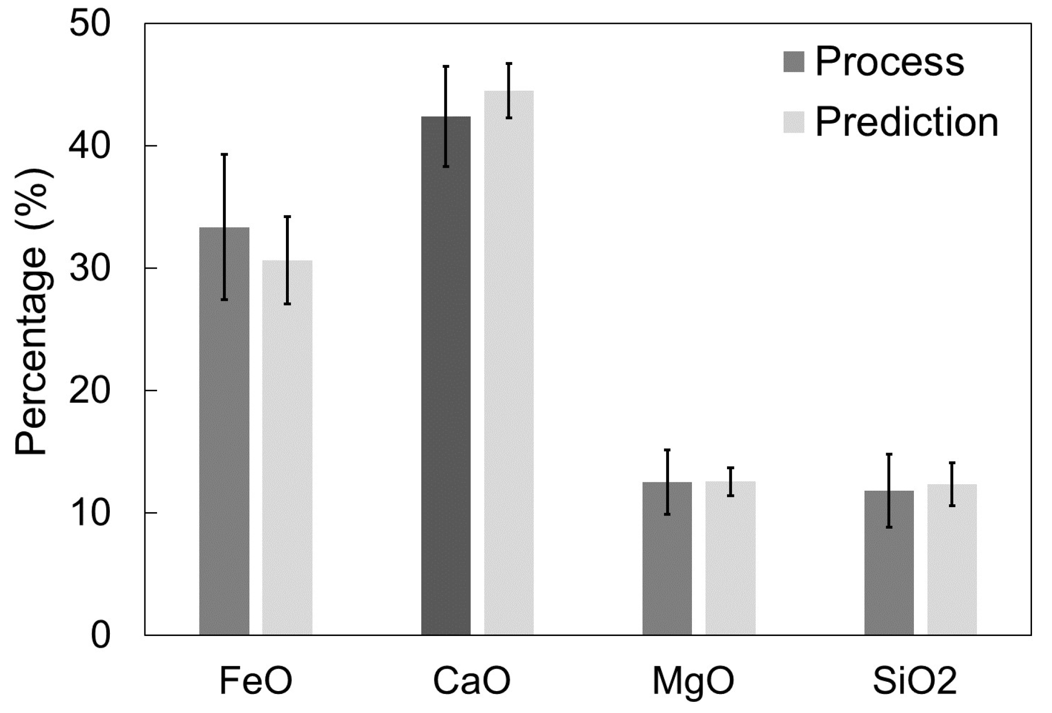
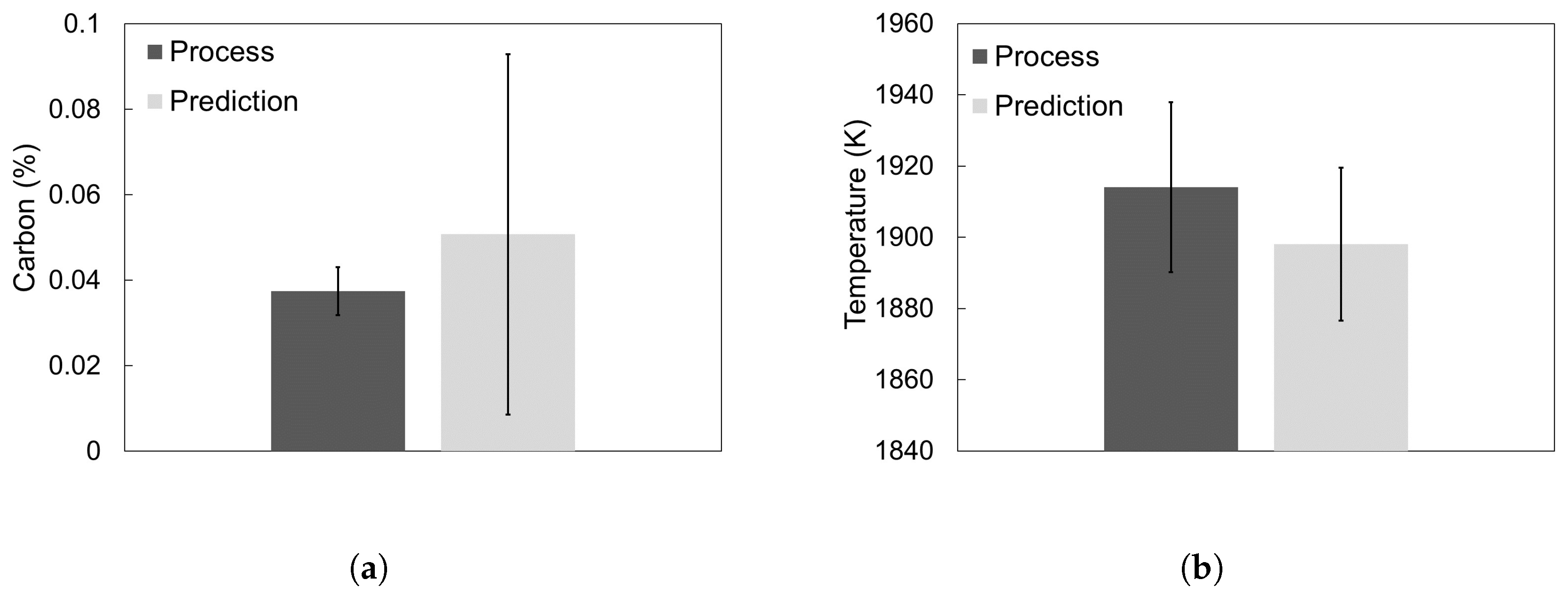
3.3. Simulation Results for Plant A Operations

The developed framework model was also used to simulate 71 heats using the data provided by Plant A for its BOF operation. The model parameters, shown in Table 1, were manually adjusted based on data collected at the end of the blow for the end-point carbon content, slag composition and temperature. The extreme conditions in the BOF often prevent samples from being collected during the blow, therefore there is no data regarding the state of the system during the blow.
The goodness of the prediction was evaluated in terms of the average of the model predictions and process data for the 71 heats. Figure 12 shows the quality of the prediction for the end-point slag composition together with the standard deviation. The results indicate that the model is able to predict the slag composition at the end of the blow reasonably well.
The carbon content of the metal bath can be measured using a carbon probe before tapping, or a sample is collected and the measurement is done in a laboratory setting, with the second giving the more accurate results. However, laboratory results are not available for all the heats for the current study. The average end-point carbon content and temperature measured using the probe and the model’s prediction for the 71 batches are shown in Figure 13, based on which it is possible to conclude that the model performs fairly well. The model was able to predict the end-point carbon content of 80% of the heats with a precision of ±0.03%, and the end-point temperature of 61% of the heats with a precision of ±30 K.
The prediction error can be attributed to several factors. If the furnace is used back-to-back, there is always some slag left over from one heat to another, however its temperature and mass are not measured and the initial mass of slag present in the system is not accurately known. Moreover, the initial temperature of the hot metal charged to the furnace is also not precisely known since it is measured, on average, 40 minutes before the blow starts. Furthermore, due to the lack of data, it is assumed that all scrap types have similar properties, which can lead to inaccurate prediction of the heat needed for complete melting. Another potential reason could be the assumption that the off-gas and slag have the same temperature; however, the data available is not sufficient to estimate the actual off-gas temperature during the process. This, with the absence of sub-models to account for phosphorus oxidation, manganese oxidation and the formation of higher iron oxides, can explain the poorer performance of the model in predicting the end-point temperature.
For each heat, the mass of iron ore, flux, scrap and hot metal charged to the furnace is different, explaining the variation in the predicted and measured values. Since the inputs are always changing, it makes it challenging to identify the primary source for larger deviations between the simulated and actual data. Plant A has three different input profiles for the oxygen flow rate and lance height, however the overall quality of the predictions is not significantly affected by the different control profiles indicating that the model can potentially be used to simulate a wide range of operating conditions.
The trajectories for the temperature, carbon content and slag composition are shown in Figure 14 for one of the heats. We observe that the trajectories are similar to the Cicutti case. The content of SiO 2 is lower for Plant A operation at the beginning of the blow because no gravel is added. Moreover, the rate of silicon oxidation is slower due to the lack of bottom stirring. As mentioned before, at low SiO 2 contents, decarburization in the emulsion is enhanced due to the reduced slag viscosity. This is evident in Figure 14a by the larger difference between the carbon content of the droplets and the carbon content of the metal bath at high FeO contents at the beginning of the blow. As expected, due to the lack of bottom stirring, the FeO content of the slag increases much faster than that for Cicutti’s case toward the end of the blow. The rapid increase can also be explained by the higher lance height towards the end of the blow compared to the mid-blow. The scaled control profiles for the oxygen flow rate and lance height for the given heat are shown in Figure 9b.
Figure 14 indicates that the model is able to predict the end-point carbon content, silicon content and temperature of liquid metal reasonably well. It also provides insights about the trajectory followed by the variables and how the change in one or more of the inputs affects the system. The developed framework could potentially aid in finding more profitable operation modes as well as in understanding the more complex relationships between process variables.

4. Conclusions

The dynamic mathematical model presented in this study extends the work of Dogan et al. [6] by incorporating slag formation and energy balances. The models for the decarburization in the emulsion zone and scrap melting were updated with more recent findings, and an empirical relationship to calculate the calcium oxide saturation was obtained. Therefore, the main phenomena taking place in the BOF were accounted for, making the model suitable for further studies.
The mathematical model was translated as a DAE system to an open source environment (Python with CasADi [12]). The current implementation allowed for a significantly shorter simulation time compared with previous studies [6,8,9]. Moreover, as more complex and detailed models for the phenomena taking place in the BOF are developed, they can be incorporated relatively easily using the current framework.
It was shown that the updated model gives a better prediction of the carbon content trajectory for Cicutti et al. [13]’s data compared with the previous version, and more recently developed dynamic models for the BOF [8,9]. The dynamic model was also used to simulate 71 heats for a real industrial BOF operation. The model predictions for the end-point carbon content, slag composition and temperature agree reasonably well with the data for a wide range of operating conditions.

Author Contributions

Conceptualization, D.D., C.S and N.D.; Methodology, D.D., C.S and N.D.; Software, D.D.; Validation, D.D., C.S. and N.D.; Formal Analysis, D.D., C.S. and N.D.; Investigation, D.D., C.S. and N.D.; Resources, D.D., C.S. and N.D.; Data Curation, D.D.; Writing – Original Draft Preparation, D.D.; Writing – Review & Editing, D.D., C.S. and N.D.; Visualization, D.D.; Supervision, C.S. and N.D.; Project Administration, C.S. and N.D.; Funding Acquisition, C.S. and N.D. All authors have read and agreed to the published version of the manuscript.

Funding

This research was funded by OCE (Ontario Centres of Excellence), Praxair, McMaster Steel Research Center (SRC) and McMaster Advanced Control Consortium (MACC).

Acknowledgments

We thank Ameya Kadrolkar for making the model for droplet decarburization available for this work. We are also grateful to Eugene Pretorious and John Thomson for helpful discussions and valuable suggestions.

Conflicts of Interest

The authors declare no conflict of interest.

References

  1. World Steel Association. Fact Sheet: Steel and Raw Materials. 2016. Available online: https://www.worldsteel.org/publications/fact-sheets.html (accessed on 27 March 2019).
  2. Molloseau, C.; Fruehan, R. The reaction behavior of Fe-CS droplets in CaO-SiO 2-MgO-FeO slags. Metall. Mater. Trans. B 2002, 33, 335–344. [Google Scholar] [CrossRef]
  3. Chen, E.; Coley, K.S. Kinetic study of droplet swelling in BOF steelmaking. Ironmaking Steelmaking 2010, 37, 541–545. [Google Scholar] [CrossRef]
  4. Jalkanen, H. Experiences in physicochemical modelling of oxygen converter process (BOF). Adv. Process. Met. Mater. 2006, 2, 541–554. [Google Scholar]
  5. Kattenbelt, C.; Roffel, B. Dynamic modeling of the main blow in basic oxygen steelmaking using measured step responses. Metall. Mater. Trans. B 2008, 39, 764–769. [Google Scholar] [CrossRef] [Green Version]
  6. Dogan, N.; Brooks, G.A.; Rhamdhani, M.A. Comprehensive model of oxygen steelmaking part 1: Model development and validation. ISIJ Int. 2011, 51, 1086–1092. [Google Scholar] [CrossRef] [Green Version]
  7. Lytvynyuk, Y.; Schenk, J.; Hiebler, M.; Sormann, A. Thermodynamic and Kinetic Model of the Converter Steelmaking Process. Part 1: The Description of the BOF Model. Steel Res. Int. 2014, 85, 537–543. [Google Scholar] [CrossRef]
  8. Sarkar, R.; Gupta, P.; Basu, S.; Ballal, N.B. Dynamic modeling of LD converter steelmaking: Reaction modeling using Gibbs’ free energy minimization. Metall. Mater. Trans. B 2015, 46, 961–976. [Google Scholar] [CrossRef]
  9. Rout, B.K.; Brooks, G.; Rhamdhani, M.A.; Li, Z.; Schrama, F.N.; Sun, J. Dynamic Model of Basic Oxygen Steelmaking Process Based on Multi-zone Reaction Kinetics: Model Derivation and Validation. Metall. Mater. Trans. B 2018, 49, 537–557. [Google Scholar] [CrossRef] [Green Version]
  10. Kadrolkar, A.; Dogan, N. The Decarburization Kinetics of Metal Droplets in Emulsion Zone. Metall. Mater. Trans. B 2019, 50, 2912–2929. [Google Scholar] [CrossRef]
  11. Shukla, A.K.; Deo, B.; Robertson, D.G.C. Scrap Dissolution in Molten Iron Containing Carbon for the Case of Coupled Heat and Mass Transfer Control. Metall. Mater. Trans. B 2013, 44, 1407–1427. [Google Scholar] [CrossRef]
  12. Andersson, J.A.E.; Gillis, J.; Horn, G.; Rawlings, J.B.; Diehl, M. CasADi—A software framework for nonlinear optimization and optimal control. Math. Program. Comput. 2019, 11, 1–36. [Google Scholar] [CrossRef]
  13. Cicutti, C.; Valdez, M.; Pérez, T.; Petroni, J.; Gomez, A.; Donayo, R.; Ferro, L. Study of slag-metal reactions in an LD-LBE converter. In Proceedings of the 6th International Conference on Molten Slags, Fluxes and Salts, Helsinki, Finland, 12–17 June 2000. [Google Scholar]
  14. Deo, B.; Boom, R. Fundamentals of Steelmaking Metallurgy; Prentice Hall International: Upper Saddle River, NJ, USA, 1993. [Google Scholar]
  15. Koria, S.C.; Lange, K.W. Penetrability of impinging gas jets in molten steel bath. Steel Res. 1987, 58, 421–426. [Google Scholar] [CrossRef]
  16. Kitamura, S.y.; Kitamura, T.; Shibata, K.; Mizukami, Y.; Mukawa, S.; Nakagawa, J. Effect of stirring energy, temperature and flux composition on hot metal dephosphorization kinetics. ISIJ Int. 1991, 31, 1322–1328. [Google Scholar] [CrossRef]
  17. Rout, B.K.; Brooks, G.; Rhamdhani, M.A.; Li, Z.; Schrama, F.N.; Overbosch, A. Dynamic Model of Basic Oxygen Steelmaking Process Based on Multizone Reaction Kinetics: Modeling of Decarburization. Metall. Mater. Trans. B 2018, 49, 1022–1033. [Google Scholar] [CrossRef]
  18. O’Malley, R.J. The Heating and Melting of Metallic DRI Particles in Steelmaking Slags. Ph.D. Dissertation, Massachusetts Institute of Technology, Cambridge, CA, USA, 1983. [Google Scholar]
  19. Zhang, L. Modeling on melting of sponge iron particles in iron-bath. Steel Res. 1996, 67, 466–474. [Google Scholar] [CrossRef]
  20. Pineda-Martínez, E.; Hernández-Bocanegra, C.A.; Conejo, A.N.; Ramirez-Argaez, M.A. Mathematical Modeling of the Melting of Sponge Iron in a Bath of Non-reactive Molten Slag. ISIJ Int. 2015, 55, 1906–1915. [Google Scholar] [CrossRef] [Green Version]
  21. Shukla, A.K. Dissolution of Steel Scrap in Molten Metal During Steelmaking. Ph.D. Dissertation, Indian Institute of Technology, Kanpur, India, 2011. [Google Scholar]
  22. Dogan, N. Mathematical Modelling of Oxygen Steelmaking. Ph.D. Dissertation, Swinburne University of Technology, Melbourne, Australia, 2011. [Google Scholar]
  23. Caffery, G.; Rafiei, P.; Honeyands, T.; Trotter, D.; Marketing, B.B. Understanding the Melting Characteristics of HBI in Iron and Steel Melts. In Proceedings of the Asssociation for Iron & Steel Technology, Nashville, TN, USA, 15–17 September 2004; Volume 1, p. 503. [Google Scholar]
  24. Gaye, H.; Wanin, M.; Gugliermina, P.; Schittly, P. Kinetics of scrap dissolution in the converter: Theoretical model and plant experimentation. In Proceedings of the 68th Steelmaking Conference, Detroit, MI, USA, 14–17 April 1985; pp. 91–103. [Google Scholar]
  25. MacRosty, R.D.; Swartz, C.L. Dynamic optimization of electric arc furnace operation. AIChE J. 2007, 53, 640–653. [Google Scholar] [CrossRef]
  26. Bekker, J.G.; Craig, I.K.; Pistorius, P.C. Modeling and Simulation of an Electric Arc Furnace Process. ISIJ Int. 1999, 39, 23–32. [Google Scholar] [CrossRef] [Green Version]
  27. Dogan, N.; Brooks, G.A.; Rhamdhani, M.A. Kinetics of flux dissolution in oxygen steelmaking. ISIJ Int. 2009, 49, 1474–1482. [Google Scholar] [CrossRef] [Green Version]
  28. Hamano, T.; Horibe, M.; Ito, K. The dissolution rate of solid lime into molten slag used for hot-metal dephosphorization. ISIJ Int. 2004, 44, 263–267. [Google Scholar] [CrossRef]
  29. Umakoshi, M.; Mort, K.; Kawai, Y. Dissolution rate of burnt dolomite in molten FetO-CaO-SiO2 slags. Trans. Iron Steel Inst. Jpn. 1984, 24, 532–539. [Google Scholar] [CrossRef]
  30. Kadrolkar, A.; Andersson, N.Å.; Dogan, N. A Dynamic Flux Dissolution Model for Oxygen Steelmaking. Metall. Mater. Trans. B 2017, 48, 99–112. [Google Scholar] [CrossRef]
  31. Subagyo; Brooks, G.A.; Coley, K.S.; Irons, G.A. Generation of Droplets in Slag-Metal Emulsions through Top Gas Blowing. ISIJ Int. 2003, 43, 983–989. [Google Scholar] [CrossRef] [Green Version]
  32. Hindmarsh, A.C.; Brown, P.N.; Grant, K.E.; Lee, S.L.; Serban, R.; Shumaker, D.E.; Woodward, C.S. SUNDIALS: Suite of nonlinear and differential/algebraic equation solvers. ACM Trans. Math. Softw. 2005, 31, 363–396. [Google Scholar] [CrossRef]
  33. Lytvynyuk, Y.; Schenk, J.; Hiebler, M.; Sormann, A. Thermodynamic and kinetic model of the converter steelmaking process. Part 2: The model validation. Steel Res. Int. 2014, 85, 544–563. [Google Scholar] [CrossRef]
  34. Brooks, G.; Pan, Y.; Subagyo; Coley, K. Modeling of trajectory and residence time of metal droplets in slag–metal–gas emulsions in oxygen steelmaking. Metall. Mater. Trans. B 2005, 36, 525–535. [Google Scholar] [CrossRef]
  35. Rout, B.K.; Brooks, G.; Subagyo; Rhamdhani, M.A.; Li, Z. Modeling of droplet generation in a top blowing steelmaking process. Metall. Mater. Trans. B 2016, 47, 3350–3361. [Google Scholar] [CrossRef] [Green Version]
  36. Mills, K.C. Viscosities of Molten Slags in Slag Atlas, 2nd ed.; Verlag Stahleisen: Düsseldorf, Germany, 1995; p. 353. [Google Scholar]
Figure 1. Schematic representation of the Basic Oxygen Furnace (BOF).
Processes 08 00483 g001
Figure 2. Material flow in the BOF assumed for the current study.
Processes 08 00483 g002
Figure 3. Schematic representation of the melting of scrap. (a) Schematic representation of a plate. (b) Schematic representation of temperature gradient between hot metal and a cold metal plate.
Processes 08 00483 g003
Figure 4. ( % C a O s a t ) obtained using the Cell Model and Equation (43) for the Cicutti et al. [13] slag data.
Processes 08 00483 g004
Figure 5. Droplet decarburization.
Processes 08 00483 g005
Figure 6. Comparison of final carbon content of metal droplets in the emulsion reported by Cicutti et al. [13], and the values predicted using Kadrolkar and Dogan [10]’s first-principles model and Equation (47) as a function of blow time.
Processes 08 00483 g006
Figure 7. (a) Comparison between measured [13] and predicted values for the temperature of liquid metal and slag. (b) Comparison between measured [13] and predicted values for the carbon content of liquid metal and the returning metal droplets.
Processes 08 00483 g007
Figure 8. (a) Total decarburization rate and decarburization rate at the emulsion zone and (b) composition of the off-gas stream exiting the BOF.
Processes 08 00483 g008
Figure 9. (a) Control profile for Cicutti et al. [13]’s data and (b) scaled control profiles for a heat from Plant A.
Processes 08 00483 g009
Figure 10. Evolution of slag composition for the Cicutti data [13] and model prediction: (a) FeO, (b) SiO2, (c) CaO, (d) MgO.
Processes 08 00483 g010
Figure 11. Comparison of the carbon content prediction by different models [6,8,9] and the measured values [13] for a 200-ton furnace.
Processes 08 00483 g011
Figure 12. Average process and predicted values for the end-point slag composition in weight percentage.
Processes 08 00483 g012
Figure 13. Average and standard deviation of the model predictions and process data for the end-point (a) carbon content of the liquid metal and (b) temperature of the liquid metal.
Processes 08 00483 g013
Figure 14. Evolution of: (a) Carbon content of liquid metal and final carbon content CC,f of the metal droplets, (b) silicon content of liquid metal, (c) slag and metal bath temperature and (d) slag composition. The values have been scaled for proprietary reasons.
Processes 08 00483 g014
Table 1. The values of model parameters for simulation and optimization. The heat transfer coefficients h are given in Wm - 2 K - 1 , and α F e p is given in kgm - 2 Pa - 1 s - 1 . All the other parameters are dimensionless.
ParametersCicuttiPlant A
α l p 0.20.07
α O 2 p 11.16
α S i , C p 102
α C O 2 p 11
α C c p 33.07
α D G p 11
α F e p 7 × 10 - 6 2.0 × 10 - 5
α S i p 77
α L p 3030
α D p 2020
α μ p 0.50.5
h L , h D 10001000
h o r e 25002500
h s - b 80,00080,000
Table 2. Mass and composition of hot metal and scrap types added to the BOF, and average scrap thickness [22].
InputHot MetalHeavy ScrapLight ScrapPig IronExternal Scrap
Mass (kg)170,000357010,00012,1404284
Thickness (mm)-10025200500
C (%)40.080.084.50.05
Si (%)0.330.050.050.50.001
Mn (%)0.520.30.30.50.2
P (%)0.066----
S (%)0.015----
Table 3. Simulation time for Cicutti et al. [13]’s data required in different studies.
ModelComputerSoftwareSolution Time
Dogan et al. [6]Pentium (R) 4 CPU 3.00 GHz and 3GB of RAMScilab240 min
Sarkar et al. [8]Not givenMatlab27 min
Rout et al. [9]Intel(R) Core(TM) i5-4570 CPU @3.20 GHz and 8 GB RAMMatlab20 min
Present studyIntel(R) Core(TM) i7-7700 CPU @3.16GHz and 16.0 GB RAMPython 3.70.036 min

